Article

Prediction of Bearing Layer Depth Using Machine Learning Algorithms and Evaluation of Their Performance

1
Graduate School of Engineering and Science, Shibaura Institute of Technology, 3-7-5 Toyosu, Tokyo 135-8548, Japan
2
College of Engineering, Shibaura Institute of Technology, 3-7-5 Toyosu, Tokyo 135-8548, Japan
*
Author to whom correspondence should be addressed.
Mach. Learn. Knowl. Extr. 2025, 7(3), 69; https://doi.org/10.3390/make7030069
Submission received: 18 June 2025 / Revised: 17 July 2025 / Accepted: 18 July 2025 / Published: 21 July 2025

Abstract

In earthquake-prone areas such as Tokyo, accurate estimation of bearing stratum depth is crucial for foundation design, liquefaction assessment, and urban disaster mitigation. However, traditional methods such as the standard penetration test (SPT), while reliable, are labor-intensive and have limited spatial distribution. In this study, 942 geological survey records from the Tokyo metropolitan area were used to evaluate the performance of three machine learning algorithms, random forest (RF), artificial neural network (ANN), and support vector machine (SVM), in predicting bearing stratum depth. The main input variables included geographic coordinates, elevation, and stratigraphic category. The results showed that the RF model performed well in terms of multiple evaluation indicators and had significantly better prediction accuracy than ANN and SVM. In addition, data density analysis showed that the prediction error was significantly reduced in high-density areas. The results demonstrate the robustness and adaptability of the RF method in foundation soil layer identification, emphasizing the importance of comprehensive input variables and spatial coverage. The proposed method can be used for large-scale, data-driven bearing stratum prediction and has the potential to be integrated into geological risk management systems and smart city platforms.

1. Introduction

Accurate estimation of bearing depth is essential to ensure the safety and efficiency of foundation design, especially in urban areas where underground conditions are often complex. With the increasing availability of geotechnical survey data and advances in computing technology, machine learning has become a powerful tool to improve prediction accuracy. This study explores the application of various machine learning algorithms in predicting bearing layer depth and compares their performance using real data.
Similarly, accurate identification of areas prone to liquefaction in the Tokyo Mirai earthquake is essential for effective disaster mitigation and urban planning. Ground failure caused by liquefaction remains a major issue in the geotechnical field, and has driven the continued research on more reliable soil resistance assessment methods. Traditional methods usually rely on site-specific geotechnical information (such as the N value from a standard penetration test (SPT), fine particle content, and groundwater level) combined with seismic parameters such as peak ground acceleration, shaking duration, or earthquake magnitude [1,2,3,4,5]. However, these methods are often limited by the narrow spatial coverage of field surveys and the challenge of extrapolating local data over a wider area [6].
SPT remains the most widely used field test method in geotechnical engineering practice, providing key parameters such as N value and bearing layer depth, both of which significantly affect the liquefaction susceptibility of the site. In particular, bearing layer depth and the properties of bearing layer depth play a crucial role in the severity and manifestation of liquefaction-induced ground failure. Shallow bearing layers above saturated loose sands are more susceptible to differential settlement, lateral expansion, and bearing capacity loss during earthquakes. Therefore, accurate prediction of bearing layer depth can serve as an important indirect indicator of liquefaction risk, complementing traditional site response analysis. This highlights the relevance of our study in providing data-driven early hazard identification tools for earthquake-prone urban areas such as Tokyo.
Notably, the depth and characteristics of the bearing layer play a crucial role in controlling how seismic energy propagates through the soil profile. Shallow or poorly developed bearing layers are more susceptible to liquefaction-induced deformations, especially when they are underlain by loose saturated sand. Therefore, reliable prediction of the bearing layer depth can serve as an indirect but important input for liquefaction risk assessment. As shown in Figure 1, the bearing layer refers to the stratum with sufficient strength to support a building. Although field surveys are reliable, they are time-consuming, labor-intensive, and costly, limiting their feasibility for large-scale deployment.
To address these challenges, it has become increasingly important to improve prediction efficiency and spatial resolution by combining field survey data with advanced computing techniques. In recent years, advances in remote sensing and geographic information systems (GIS) have improved the description of subsurface characteristics on a larger scale [7,8]. At the same time, machine learning (ML) has emerged as a promising tool to improve prediction accuracy for geotechnical engineering applications [9]. Various ML algorithms, such as decision trees (DTs) [10], artificial neural networks (ANNs) [11], support vector machines (SVMs) [12], and random forests (RFs) [13,14], have performed well in classification and regression tasks in multiple fields, including earth science and environmental modeling [15,16,17,18,19].
Although traditional statistical modeling and empirical methods have been widely used in geotechnical engineering, these methods often rely on strong assumptions about the behavior of foundations and usually require parameter calibration under site-specific conditions. This limits their application in urban environments with complex geology and dramatic spatial variations, such as Tokyo. In contrast, machine learning methods are more suitable for automatically extracting non-linear relationships from high-dimensional, multivariate geologic data to improve the generalization ability and spatial adaptability of predictions. Although hybrid geophysics–machine learning models are theoretically advantageous, such methods usually rely on finer knowledge of soil models and customized feature design, which makes them difficult to be widely deployed. Therefore, in this study, a pure machine learning approach based on routinely available borehole data and SPT information was chosen, aiming to achieve efficient and generalizable regional depth prediction of bearing layers.
ML applications in geotechnical engineering are expanding globally [20,21,22], with RFs in particular showing high predictive performance in soil geochemistry and environmental sciences [23,24,25,26,27]. However, existing studies have rarely conducted comprehensive, quantitative comparisons of different ML algorithms using the same input variables for geotechnical prediction tasks [28,29].
In recent years, machine learning methods (e.g., support vector machine SVM, artificial neural network ANN, and random forest RF) have demonstrated good prediction ability and adaptability in a variety of complex data environments in geotechnical and materials engineering research. For example, the flexural and compressive strengths of cement mortar with chemical admixtures have been successfully predicted using SVM and ANN [30]; in addition, there is a hybrid modeling approach that integrates multiple algorithms to analyze the strength behavior of hand-mixed cement mortar under different conditions [31]. These studies have demonstrated the reliability and wide applicability of the aforementioned algorithms in the prediction of engineering material properties.
To provide a clearer picture of the current state of research on predicting bearing layer depth, Table 1 summarizes representative studies in this area. It summarizes the machine learning (ML) models used, the input features, the study locations, and the reported performance metrics. As shown in Table 1, most of the existing studies have focused on regions such as East Asia and the Middle East, usually using a single algorithmic approach. Few studies have addressed the complex geologic environment of Tokyo or conducted systematic multi-model comparisons.
Addressing this research gap, this study evaluates and compares a variety of multiple multiplicative mathematical algorithms for predicting bearing layer depths using geotechnical datasets from the Tokyo Metropolitan Area. The selected models—SVM, ANN, and RF—represent kernel-based, neural network-based, and ensemble-based approaches, respectively. These models strike a balance between prediction accuracy, computational efficiency, and interpretability and are well suited for practical geotechnical modeling tasks.
A larger and more diverse dataset, as well as a broader set of explanatory variables, was used in this study than in previous studies. This allows for a more detailed study of how spatial data density affects prediction performance. Ultimately, we aim to develop a robust and generalizable ML framework to enhance liquefaction risk assessment in Japan and to promote the development of data-driven resilient smart cities. By combining conventional field survey data with advanced computational techniques, this study aims to support sustainable urban development and improve geotechnical engineering decision-making.
The main contributions of this study are as follows:
  • A comprehensive comparative analysis of three established machine learning models (support vector machine (SVM), artificial neural network (ANN), and random forest (RF)), applied to a real geotechnical dataset in the Tokyo metropolitan area, is performed.
  • Two different input feature configurations (with and without stratigraphic classification) are integrated and their impact on the prediction performance is evaluated.
  • The robustness of the model is evaluated under different spatial data densities to simulate the uneven distribution of boreholes in the real world.
  • A practical and scalable machine learning framework is developed to support regional liquefaction risk assessment and urban infrastructure planning in data-constrained environments.

2. Study Area and Dataset Description

2.1. Overview of the Study Area

Tokyo’s topography transitions from west to east through mountainous regions, hilly terrain, plateaus, and lowlands. Figure 2 presents a micro-topographic classification map of the southwestern portion of the eastern Tokyo area and was provided by the Tokyo Geographical Research Institute. The lowland regions are predominantly underlain by thick, soft alluvial deposits, often exhibiting highly irregular basal boundaries. This complex stratigraphy is the result of significant coastal transformations driven by sea level fluctuations during glacial and interglacial periods.
Over the past 10,000 years, the coastline has advanced inland, contributing to the formation of a deltaic plain that extends across the Tokyo metropolitan area. This delta has accumulated fine sand deposits, resulting in surface strata characterized by several meters of loose sandy soils. These sandy layers typically contain 10–30% fine particles and exhibit standard penetration test (SPT) N values in the range of 5–10, indicating relatively low strength and density.
The dominant soil type in the Tokyo area is a mixture of sand, silt, and clay, which is classified as Kanto loam based on its particle size distribution. From a geotechnical perspective, undisturbed Kanto loam is moderately firm, with a porosity of approximately 3 to 4 and a relatively high natural water content, typically between 80% and 180%. However, once excavated or disturbed, the loam rapidly loses its structural strength due to its high pore-water content, transitioning into a soft, paste-like consistency. This property was a contributing factor to the widespread damage to buildings and water pipelines observed in valley-bottom areas during the 1923 Great Kanto Earthquake.
Given the variability of subsurface conditions and the significant influence of geological layering on foundation behavior, stratigraphic classification plays a critical role in accurately determining the depth of bearing layers in geotechnical investigations.
In this study, a total of 942 geotechnical survey records were utilized for model development and validation. The spatial distribution of these survey locations is illustrated in Figure 3.

2.2. Data Sources and Definitions

The primary objective of this study is to develop a predictive model for estimating the depth of the bearing layer, a fundamental concern in evaluating the vertical bearing capacity of shallow foundations. The behavior of shallow foundations in spatially variable soils has been a key topic in geotechnical engineering research over the past three decades [35,36,37].
In this study, the depth of the bearing layer is defined based on the standard penetration test (SPT) N value. The SPT is one of the most widely adopted in situ tests used for determining soil stratigraphy, type, and relative strength during geotechnical site investigations. The procedure involves driving a split-barrel sampler 460 mm into the soil at the bottom of a borehole using a 63.5 kg hammer dropped from a height of 760 mm. The number of hammer blows required to penetrate the final 300 mm (in two 150 mm increments) is recorded as the SPT N value [38]. This value provides valuable insight into subsurface conditions and is frequently used to assess bearing capacity and liquefaction resistance [39].
In general, soil layers with an N value greater than 20 are considered suitable as foundation support, while those with N values between 30 and 50 are regarded as adequate for civil and structural applications. Layers with N values exceeding 50 are typically classified as highly competent strata capable of supporting large-scale infrastructure, such as high-rise buildings [40]. In this study, a bearing layer is defined as a continuous soil layer in which the N value exceeds 50 over a depth of at least 3 m [41].
The dataset used in this study was derived from the Tokyo Geological Information Survey, and consists of borehole data collected through field-based SPTs conducted by cooperative construction and survey companies. Each data point includes N values, ground surface elevations, and stratigraphic descriptions at specific geographic locations. Since terrain variability across Tokyo affects the elevation settings and depth to competent layers, accounting for topographic and geological conditions is essential. For instance, in mountainous or uneven regions, elevation changes directly influence the measured depth to the bearing layer.
For the purpose of this analysis, the subsurface geology is simplified into two major stratigraphic classifications: alluvial layers and diluvial layers. Examples of input features and corresponding target values for three representative sites are shown in Table 2, which correspond to locations identified in Figure 3. Among the 942 geotechnical records utilized in this study, the dataset was randomly split into training, validation, and testing subsets using a 70:20:10 ratio. Although random splits may introduce some spatial leakage, this study focuses on the overall prediction performance rather than strict spatial extrapolation. To mitigate sampling bias, we repeated each experiment multiple times with different seeds and reported the average results, which showed consistent trends across model runs.

3. Machine Learning Algorithms

3.1. Overview of Applied Algorithms

In this study, three machine learning algorithms were employed to evaluate their effectiveness in predicting the depth of the bearing layer using geotechnical survey data: random forest (RF), artificial neural networks (ANNs), and support vector machines (SVMs). These algorithms were selected based on their proven capabilities in regression tasks and their ability to capture complex, non-linear patterns in geospatial and geotechnical datasets.
It should be noted that the goal of this study is not to propose a new machine learning method, but to systematically compare commonly used models within an experimental framework representative of geotechnical engineering. The methodological value of this study is reflected as follows: through performance evaluation under different input feature combinations (Case-1 and Case-2) and multiple spatial data density conditions, and the stability and practicality of the model under the limited conditions of urban regional geological exploration are explored, providing decision support for actual foundation design and disaster assessment.
This study selected three models, i.e., RF, ANN, and SVM, mainly based on their respective performance advantages and their wide application in geotechnical engineering. These three types of models represent ensemble methods, neural network methods, and kernel function methods, respectively, which are representative and suitable for comparative analysis. RF performs well in dealing with noisy data and interpretability, ANN is suitable for modeling complex non-linear relationships, and SVM has good stability under high-dimensional small sample data.
Although more advanced models such as gradient boosting (XGBoost), deep ensemble methods, or Gaussian processes have potential in predictive performance, this study focuses more on the practicality, interpretability, and engineering deployability of the models. Therefore, these three classic models were selected for systematic evaluation.
Random forest is an ensemble learning technique that constructs multiple decision trees and aggregates their outputs to generate a final prediction. It is an extension of the bagging method introduced by Breiman [42,43], and has demonstrated strong performance in managing high-dimensional, noisy data [44,45]. Due to its robustness and low sensitivity to hyperparameter tuning, RF is particularly well suited for practical engineering applications. The random forest architecture utilized in this study is illustrated in Figure 4.
Artificial neural networks (ANNs) are computational models inspired by the structure of biological neural systems. They consist of interconnected layers of neurons that can learn non-linear mappings between input features and target outputs. ANNs are highly flexible and capable of modeling complex functional relationships, making them suitable for geotechnical applications. However, their performance is highly dependent on network architecture, training algorithms, and parameter tuning [46,47]. The ANN architecture adopted in this study was implemented using the PyTorch version 2.2.0 framework and is shown in Figure 5.
Support vector machines (SVMs), originally proposed by Vapnik [48,49], are supervised learning models that aim to construct an optimal hyperplane in a transformed feature space. By utilizing kernel functions, such as the radial basis function (RBF), SVMs can effectively capture non-linear relationships, making them applicable to complex regression problems [50]. The conceptual structure of the SVM model used in this study is illustrated in Figure 6.
These three algorithms represent distinct paradigms in machine learning: ensemble-based decision trees (RF), connectionist models based on neural computation (ANN), and margin-based optimization approaches (SVM). Their differing methodological characteristics enable a comprehensive comparative analysis of performance under varying conditions, such as differences in feature composition and spatial data density. A detailed quantitative evaluation of their predictive accuracy is presented in Section 5.

3.2. Theoretical Foundations

3.2.1. Definition of Random Forest

To address complex modeling tasks, particularly those involving large and high-dimensional datasets, ensemble learning methods have been developed. One prominent ensemble approach is bootstrap aggregating, commonly referred to as bagging. Bagging was introduced by Breiman [43] as a means to reduce the variance of predictive models by aggregating the outputs of multiple base learners trained on randomly resampled subsets of the data.
Random forest (RF) is a decision-tree-based extension of the bagging method, also developed by Breiman in the early 2000s [44]. It is recognized as one of the most effective and widely used algorithms for handling complex, high-dimensional data [45]. In a random forest, multiple decision trees are constructed using different bootstrapped samples of the dataset. At each split node in a tree, a random subset of features is selected to determine the optimal split, which introduces additional randomness and helps reduce correlation between trees. For classification tasks, the final prediction is determined by majority voting across all trees; for regression tasks, the output is typically the average of all tree predictions. The architecture of the RF model used in this study is depicted in Figure 4.

3.2.2. Definition of Artificial Neural Networks

Artificial neural networks (ANNs) are mathematical models inspired by the structure and functionality of biological neural networks. They are composed of interconnected layers of neurons (or nodes), where each neuron receives weighted inputs and produces an output through an activation function. ANNs are capable of learning complex, non-linear mappings between input and output variables, making them suitable for function approximation, pattern recognition, and regression tasks [46].
During the training process, the connection weights between neurons are iteratively adjusted based on error feedback using optimization algorithms such as gradient descent. This learning continues until the model converges, typically when the change in prediction error between training epochs falls below a predefined threshold [47]. The ANN architecture used in this study, implemented using the PyTorch version 2.2.0 framework, is illustrated in Figure 5.

3.2.3. Definition of Support Vector Machines

Support vector machines (SVMs) are supervised learning models that aim to find the optimal hyperplane that separates data points in a high-dimensional feature space with the maximum margin. Originally developed by Vapnik [48,49], SVMs are capable of handling both classification and regression tasks. Their effectiveness stems from their ability to construct non-linear decision boundaries through the use of kernel functions, which implicitly map input data into a higher-dimensional space.
The most commonly used kernel in regression problems is the radial basis function (RBF) kernel. SVMs formulate learning as a convex quadratic optimization problem in which the model minimizes the sum of squared weights (to control complexity) while penalizing misclassification or prediction error within a defined tolerance. The conceptual framework of the SVM model applied in this study is presented in Figure 6.

4. Data Preprocessing and Model Development

4.1. Data Preprocessing

Following data collection, preprocessing is a crucial step to ensure the quality and suitability of the dataset for machine learning analysis. The preprocessing stage typically serves two primary purposes: (1) reducing data complexity to enhance computational efficiency, and (2) adapting the dataset to align with the requirements of the selected algorithms [51].
  • Missing Value Treatment: In this study, missing values were addressed through deletion, particularly for stratigraphic classification, which is a categorical (non-continuous) variable. Imputation was not considered appropriate due to the potential risk of introducing artificial bias into discrete geological categories.
  • Data Standardization: To ensure comparability among features with different units and magnitudes, Z-score normalization was applied. This method standardizes each attribute by centering it at zero and scaling it based on its standard deviation. The Z-score normalization transforms each feature value v i into a standardized value v i , as defined by Equations (1)–(3) [52,53]:
  • Feature Selection: To reduce dimensionality and improve model performance, a filter-based feature selection method was employed. This approach selects relevant features based on statistical characteristics independent of the learning algorithm. By eliminating irrelevant or redundant features, this process mitigates the curse of dimensionality and reduces model complexity. Feature selection was performed prior to model training.
  • Outlier Detection and Dimensionality Reduction: In addition to normalization and feature selection, we also performed outlier detection on the dataset, using exploratory data analysis (EDA) to identify extreme values in key variables such as borehole depth and SPT N value. Some abnormal records that clearly deviated from the conventional engineering range (such as typos) were removed before model training. Regarding dimensionality reduction, we considered using principal component analysis (PCA), but due to the small number of input variables and the clear geotechnical significance of each feature, all original variables were retained to enhance interpretability. We believe that methods such as PCA (such as t-SNE and UMAP) may be more valuable when dealing with high-dimensional or non-engineering semantic data and suggest further exploration in more complex data scenarios in the future.
  • Bias–Variance Trade-off: An important concept in model evaluation is the bias–variance trade-off, which explains the relationship between model complexity and prediction error. Bias refers to the difference between the expected prediction and the true value, while variance measures the fluctuation in model output due to changes in the training data. These relationships are mathematically defined by Equations (4) and (5):
v i = v i E ¯ s t d ( E )
s t d E = 1 ( n 1 ) i = 1 n ( v i E ¯ ) 2
E ¯ = 1 n i = 1 n v i   o r   m e a n   v a l u e
where v i is the normalized value, v i is the original value of the i-th element, E ¯ is the mean, and std(E) is the standard deviation of the variable E.
b i a s 2 x = ( f ¯ x y ) 2
v a r x = E D f x ; D f ¯ ( x ) 2
where x is the test sample, y is the true label, D represents the training dataset, f x ; D is the prediction function trained on D , and f ¯ ( x ) is the expected prediction. Simple models tend to have high bias and low variance, while complex models tend to exhibit low bias and high variance. A well-performing model should strike a balance between these two sources of error to minimize generalization error.

4.2. Model Configuration and Hyperparameter Tuning

4.2.1. Random Forest

The random forest (RF) algorithm was configured and optimized through a systematic hyperparameter tuning process. The procedure involved constructing an ensemble of decision trees and tuning key parameters to maximize model performance while avoiding overfitting.
  • Algorithm Configuration: To build the RF model, a bootstrap sampling procedure was repeated 91 times. In each iteration, a new sub-training set D was generated by sampling with replacement from the original training dataset. From each sub-training set, a decision tree was constructed using a randomly selected subset of input features, where the number of selected features m satisfied the condition m < 5. The resulting ensemble of 91 decision trees formed the final RF model, as illustrated in Figure 2.
  • Hyperparameter Tuning Strategy: Hyperparameter optimization was performed in two stages: first, by tuning the parameters related to the bagging framework (i.e., the ensemble level) and second, by tuning the parameters associated with the individual decision trees. During each tuning step, other parameters were held constant to isolate the effect of the target parameter.
    (1)
    Number of Estimators (n_estimators): This parameter controls the number of decision trees in the ensemble. A grid search was conducted over the range 1 to 101 with a step size of 10. Ten-fold cross-validation was used to evaluate model performance. The optimal value was determined to be 91, yielding a prediction accuracy of 98.0%, which was a substantial improvement over the default setting (accuracy: 93.7%).
    (2)
    Maximum Number of Features (max_features): With n_estimators = 91, the maximum number of features considered for splitting at each tree node was optimized in the range of 1 to 5. The best-performing value, selected based on cross-validation accuracy, was 5, indicating that using all available features at each split yielded the highest performance.
The final set of hyperparameters used in the RF model is summarized in Table 3. Key parameters are defined as follows:
  • n_estimators: Number of decision trees in the forest. Too few trees may lead to underfitting, while too many trees provide diminishing returns and increased computation time.
  • max_depth: Maximum depth of each decision tree. When set to None, the trees are expanded until all leaves are pure or contain fewer samples than the minimum threshold. Limiting depth is recommended for large datasets with many features.
  • max_features: Number of features considered for the best split. A higher value increases model complexity but may improve accuracy.
  • bootstrap: Boolean parameter indicating whether sampling is performed with replacement (True enables bootstrap sampling).
  • oob_score: Boolean parameter indicating whether out-of-bag (OOB) samples are used to estimate generalization performance.
All parameter selections were validated using ten-fold cross-validation to ensure robustness and to prevent overfitting.

4.2.2. Artificial Neural Networks

The artificial neural network (ANN) model used in this study was developed using the PyTorch version 2.2.0 deep learning framework. The model construction and training process consisted of the following steps: (1) dataset preparation, (2) model architecture definition, (3) loss function and optimizer selection, (4) model training, (5) model evaluation, and (6) hyperparameter tuning.
The input layer consists of five input neurons, corresponding to the selected explanatory variables, and a single output neuron representing the predicted bearing layer depth. The objective of the network is to learn a mapping from input features to output values by adjusting the weights of the connections between neurons to minimize the prediction error.
To capture non-linear relationships in the data, three hidden layers were incorporated into the model, with 256, 128, and 64 neurons, respectively. The ReLU (Rectified Linear Unit) function was employed as the activation function for all hidden layers to introduce non-linearity. Batch normalization (BatchNorm1d) was applied after each hidden layer to stabilize training and improve convergence speed.
The model was trained using a learning rate of 0.0001, with training epochs set to 500 and 1000 in different experimental settings for performance comparison. The final architecture and training configuration are summarized in Table 4.
The loss function used during training was the mean squared error (MSELoss), which is suitable for continuous regression tasks. The Adam optimizer was chosen because of its adaptive learning capability, and the β parameter was left as default. The batch size was 32 for all experiments. No dropout or early stopping was used in this study so that full convergence was achieved within the specified number of epochs. A fixed random seed (42) was set before training to ensure reproducibility.
The ANN architecture (256–128–64) and its training configuration used in this study were determined based on preliminary experimental results to achieve a balance between model performance and training stability. We explored different combinations of hidden layer sizes and learning rates by combining five-fold cross-validation with manual grid search. Although dropout and early stopping were not enabled in the final experiment, dropout (0.3) and early stopping (10 rounds were tolerated) were tried in the early tests, but the performance improvement was limited under the premise of a small model structure and controlled dataset. In addition, the He normal initialization method was used for the initialization of neural network parameters to adapt to the ReLU activation function and promote convergence stability.
We also acknowledge that more advanced parameter adjustment strategies such as Bayesian optimization and nested cross-validation may further improve the prediction performance but, considering the computational resource limitations of the current study, they have not been adopted. This part has been listed as a future improvement direction in the discussion.

4.2.3. Support Vector Machines

The support vector machine (SVM) algorithm follows a structured process consisting of four main stages: (1) data preprocessing, (2) feature mapping via kernel transformation, (3) hyperplane construction, and (4) prediction. After normalizing the input features, a kernel function is applied to project the data into a high-dimensional feature space. In this space, the algorithm seeks to determine an optimal hyperplane that maximizes the margin between different classes or regression targets.
The kernel function plays a central role in SVMs by enabling the modeling of non-linear relationships through implicit high-dimensional transformations. Among various kernel types, this study adopts the radial basis function (RBF) kernel due to its effectiveness and widespread application in non-linear regression tasks. The RBF kernel requires extensive computation, including matrix operations and exponential functions, to evaluate similarity in the transformed space.
To optimize the SVM model, a grid search combined with cross-validation was used to identify the best hyperparameter settings. The two key hyperparameters tuned in this process are:
  • C: The regularization parameter that controls the trade-off between minimizing training error and maintaining model generalization.
  • Gamma (γ): The kernel coefficient that determines the influence range of a single training example in the RBF kernel.
In this study, C was fixed at 1, while γ was varied from 0.001 to 1 in increments of 0.1. The optimal combination of parameters was selected based on cross-validation accuracy, and the final SVM model was trained using these optimal values. Before model training, all input features were normalized to the range [0, 1] using MinMaxScaler. During hyperparameter tuning, we used a ten-fold cross-validation strategy to evaluate model performance. Although multiple values of the regularization parameter C were tested in preliminary experiments, the model showed the most stable and best generalization performance when C = 1, so it can be adopted and this value treated as a fixed value. The model performed best when γ = 0.3, which achieved the best balance between local sensitivity and model smoothness. The detailed configuration and hyperparameters of the SVM model are summarized in Table 5.

5. Results and Discussion

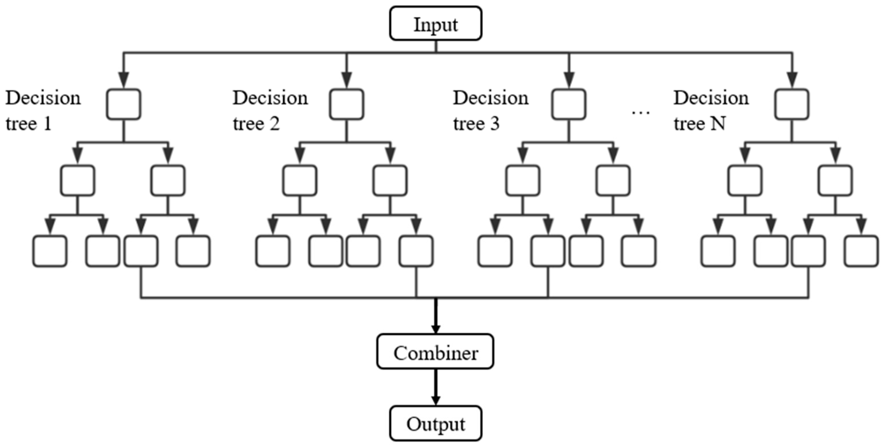
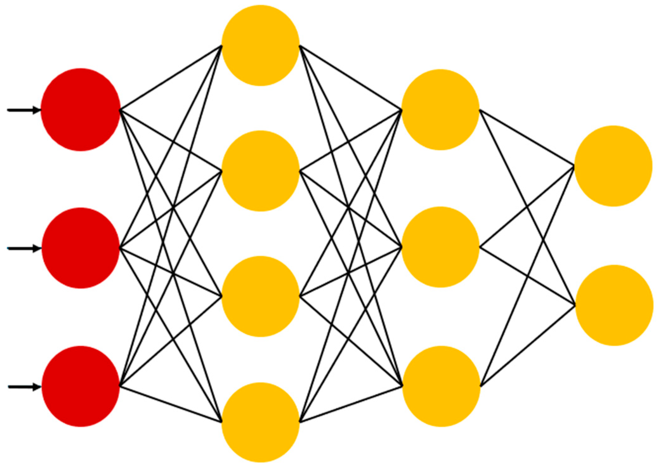
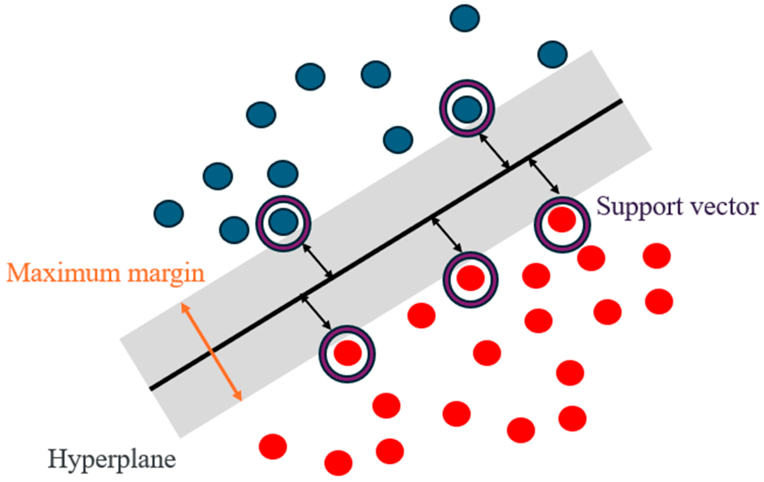
The trained models based on the three machine learning algorithms, random forest (RF), artificial neural networks (ANNs), and support vector machines (SVMs), were applied to perform predictive analysis of bearing layer depth. Two experimental cases were defined based on the set of explanatory variables used:
  • Case-1: Latitude, longitude, and elevation were used as explanatory variables;
  • Case-2: Latitude, longitude, elevation, and stratigraphic classification were used as explanatory variables.
In both cases, the target variable was the depth of the bearing layer.
Input features were selected based on their availability in the borehole dataset and their relevance to the subsurface stratigraphy. In Case 2, stratigraphic classification was incorporated into a set of binary variables (0/1) indicating the presence or absence of a particular dominant soil type (e.g., clay, sand, or gravel) in each borehole record. This coding approach was adopted because detailed lithologic descriptions were inconsistent across the dataset, making more fine-grained or ordinal coding impractical. While richer categorical descriptors such as lithologic codes or depositional environments could provide additional insights, these data are not complete or standardized. We acknowledge that this is a limitation, and future research may explore the use of one-hot encoding or embedded categorical features.

5.1. Evaluation of Prediction Accuracy

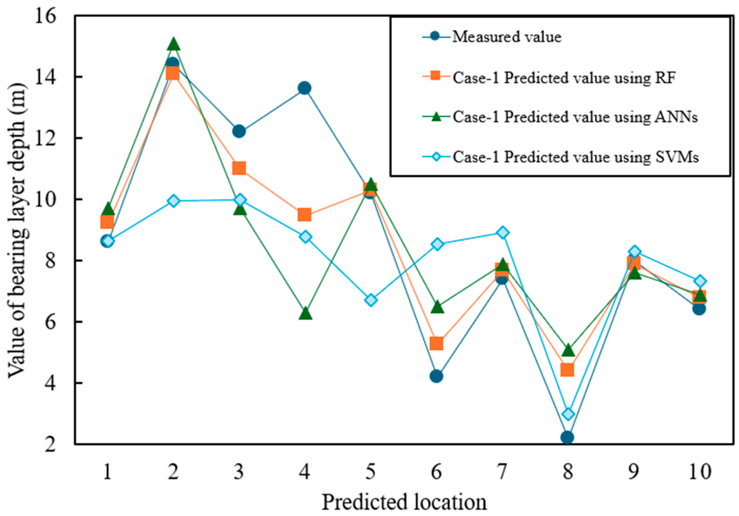
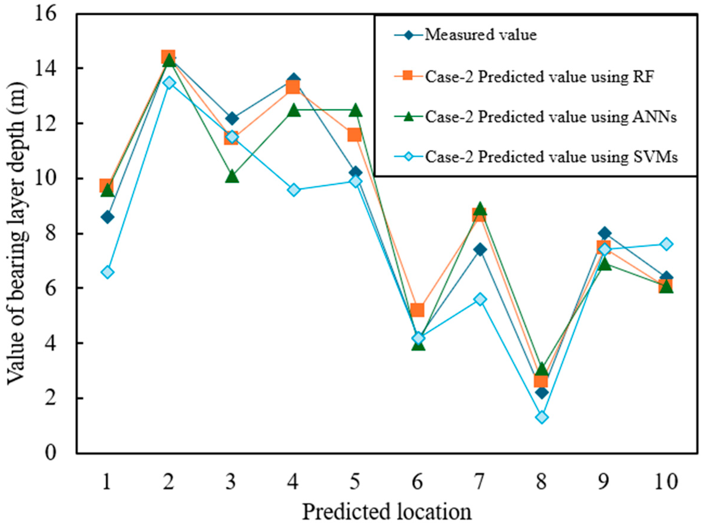
For performance evaluation, the trained models were used to predict the bearing layer depth at 10 randomly selected locations in Tokyo. The predictions were compared against actual measured data at these sites, and the prediction errors were computed.
Figure 7 and Figure 8 show the prediction results for Case-1 and Case-2, respectively, where the horizontal axis represents the predicted values and the vertical axis represents the measured values. The numerical results are summarized in Table 6, which presents three widely used error metrics:
  • Mean absolute error (MAE): The average of the absolute differences between predicted and actual values;
  • Mean squared error (MSE): The average of the squared differences between predicted and actual values. Lower MSE values indicate a better model fit;
  • Root mean squared error (RMSE): The square root of MSE. Larger RMSE values suggest a greater overall error.
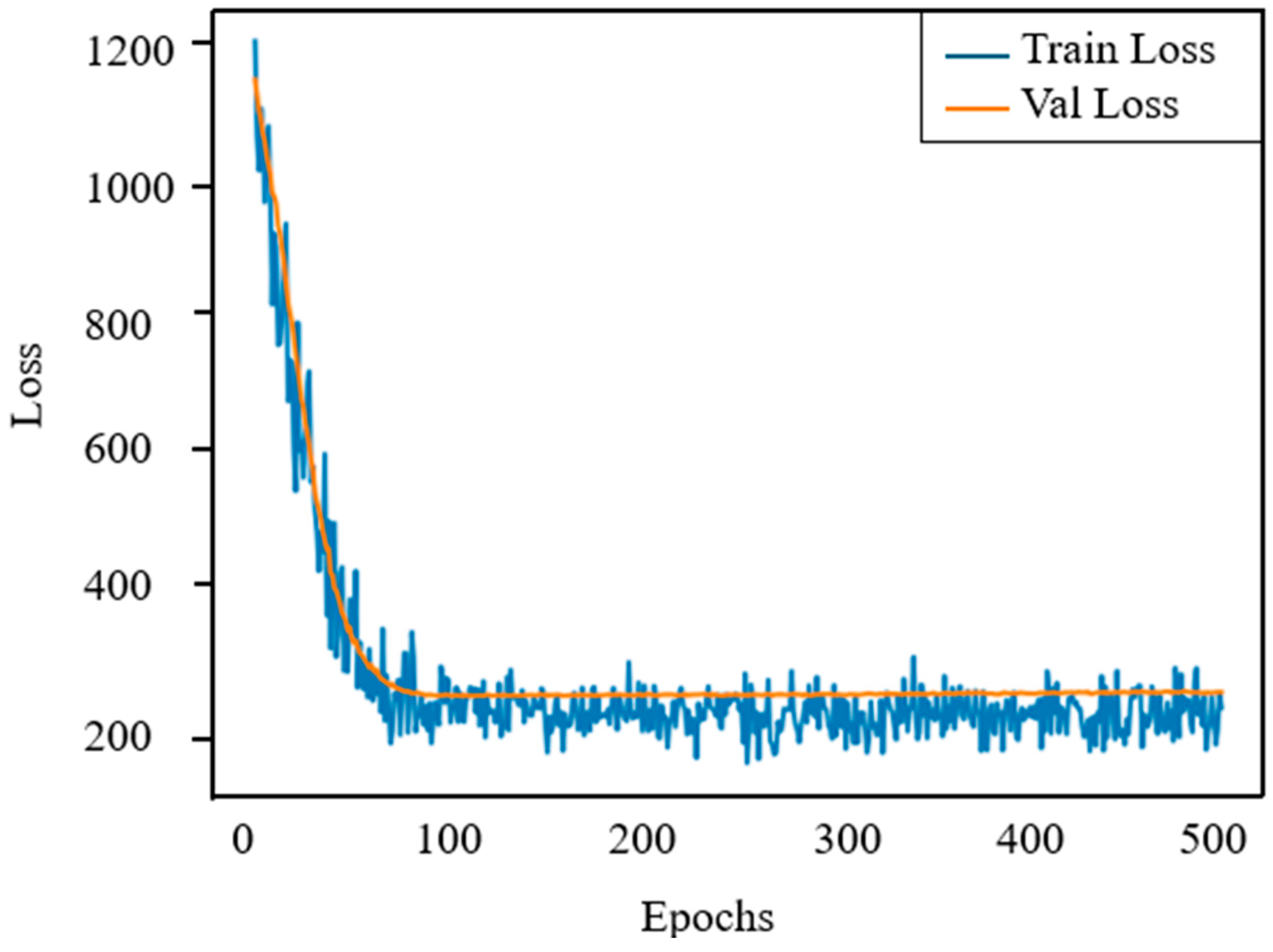
In terms of model performance, random forests consistently outperform ANNs and SVMs in terms of accuracy and robustness. However, to better understand the training behavior of ANNs and address overfitting, we plotted the training and validation loss curves, as shown in Figure 9. The figure shows that both losses drop rapidly within the first 100 epochs, indicating fast convergence. After about 120 epochs, the curves stabilize and remain closely aligned, with a small gap between the two. This indicates that the model has good generalization capabilities to unseen data and no significant signs of overfitting. The observed stability confirms the effectiveness of the selected network architecture and training settings, including learning rate, batch normalization, and batch size. Overall, while ANNs are more sensitive to hyperparameter settings than random forests (RFs), the loss curve analysis provides quantitative evidence that the network has been properly regularized and maintains strong generalization capabilities.
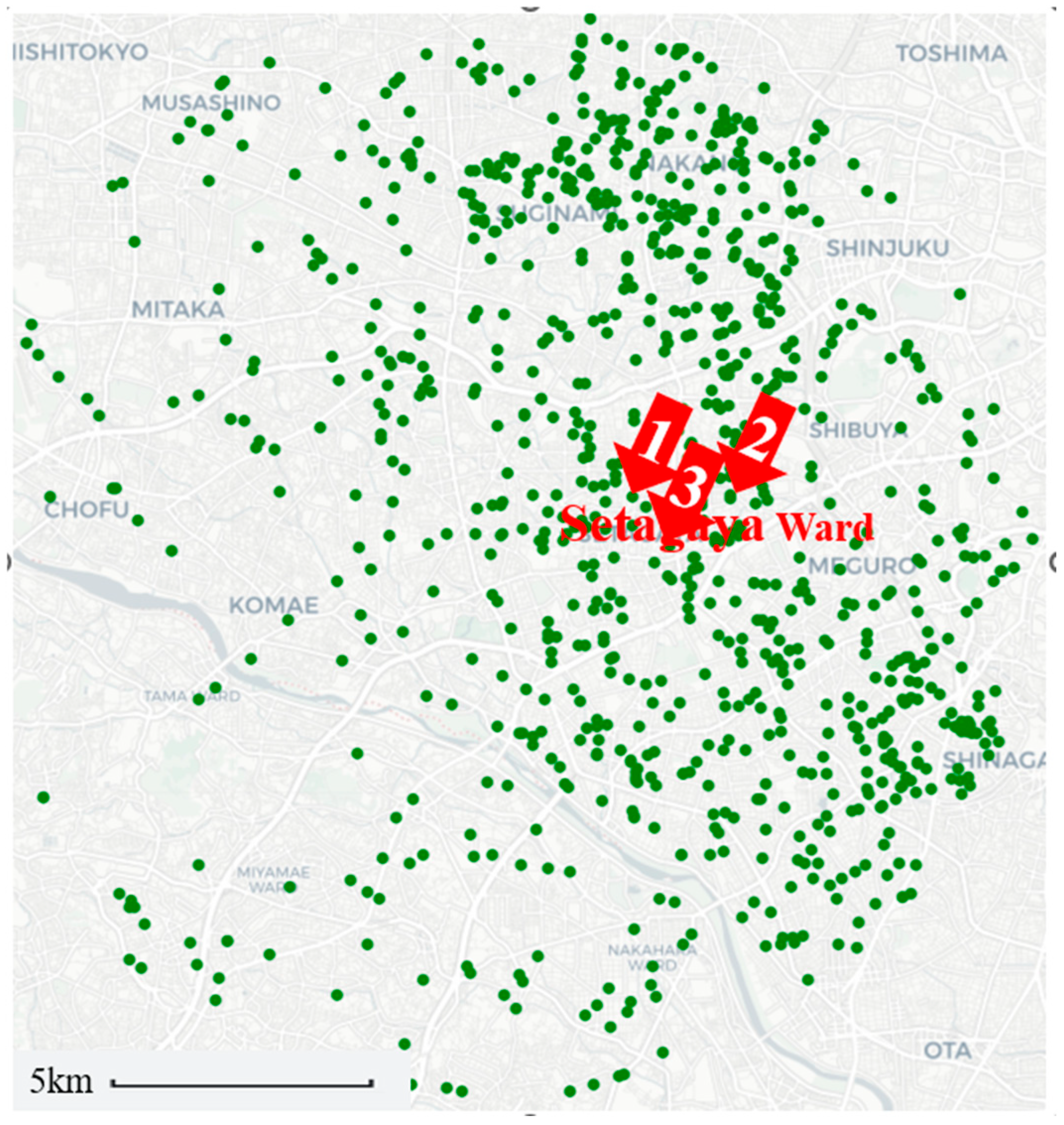
Table 7 presents the detailed prediction outcomes for the three representative locations highlighted in Figure 3.
The results indicate that random forest consistently outperformed ANNs and SVMs in both cases. This superior performance is attributed to the robustness of RF, which is relatively insensitive to hyperparameter tuning and less prone to overfitting. In contrast, the performance of ANNs and SVMs exhibited greater variability, likely due to challenges in identifying optimal parameters, particularly under the influence of discretized feature spaces and limited data.
In terms of model-specific limitations, support vector machines (SVMs) are highly sensitive to kernel function and parameter selection and are computationally expensive for large datasets. Artificial neural networks (ANNs) require large amounts of training data to avoid overfitting, and their performance is affected by the choice of initialization strategy and learning rate. Random forest (RF) models, while robust, can suffer from feature selection bias in high-dimensional or sparse input spaces, and their ensemble nature reduces model interpretability.
Moreover, the inclusion of additional explanatory variables, as in Case-2, led to improved prediction accuracy across all models. This can be explained by two main factors:
(1)
Enhanced Data Representation: The inclusion of stratigraphic classification as an additional feature enabled the models to better capture geological characteristics and underlying patterns relevant to bearing layer depth.
(2)
Feature Interactions: Additional features increase the potential for discovering meaningful interactions among variables, allowing the models to build more accurate and expressive predictive functions.
However, while increasing the number of explanatory variables can enhance predictive performance, it may also increase the risk of overfitting, especially when irrelevant or redundant features are included. Therefore, careful feature selection is essential to balance model complexity and generalization ability.
For the random forest (RF) model, we evaluated the impact of varying the number of estimators (n_estimators) and the number of features considered at each split (max_features). The number of trees tested ranged from 10 to 150, increasing in increments of 10. The results show that the model performance improves rapidly when the number of trees reaches about 90, after which the improvement levels off, indicating diminishing returns. Similarly, max_features ranged from 1 to 5. The best results were observed when max_features was set to 5, meaning that the best performance was achieved using all input features at each node split. Overall, the RF model showed relatively low sensitivity to changes in hyperparameters, demonstrating its robustness.
For artificial neural networks (ANNs), we performed sensitivity analyses on the number of neurons in the hidden layer and the learning rate, two key hyperparameters that directly impact model complexity and training dynamics. We varied the number of neurons in the first hidden layer from 32 to 512 and tested learning rates ranging from 0.00001 to 0.01. Results show that both parameters significantly impact model performance. Specifically, a learning rate of 0.0001 consistently achieves stable convergence with the lowest error across multiple configurations. Too small a learning rate results in slow convergence, while too large a learning rate leads to instability and divergence during training. Similarly, too few neurons limits the capacity of the model, while too many leads to overfitting. These findings highlight the need to carefully tune ANN models.
To evaluate the sensitivity of the support vector machine (SVM) model, we investigated the impact of the kernel coefficient γ. This coefficient plays a crucial role in determining the shape of the decision boundary when using the radial basis function (RBF) kernel. The value of γ was varied from 0.001 to 1.0 in increments of 0.1, while the regularization parameter C was fixed to 1. The results show that the model performance fluctuates significantly within this range. Specifically, γ values between 0.2 and 0.4 produce the lowest RMSE and MAE, while values outside this range lead to increased prediction errors due to overfitting (larger γ) or underfitting (smaller γ). This shows that the SVM model is highly sensitive to the choice of kernel parameters.
In order to enhance the interpretability and reliability of the model in practical engineering, this study introduces a prediction uncertainty quantification method based on the traditional error assessment metrics (MAE, MSE, and RMSE) to provide a more comprehensive basis for model evaluation.
For the RF model, we used the Quantile Regression Forests (QRF) method to obtain the 95% prediction interval (PI) corresponding to each predicted value. This method can effectively estimate the upper and lower confidence bounds based on the distribution information of the nodes in the tree model.
For the SVM and ANN models, since they do not have built-in confidence outputs, we estimate the model uncertainty by the bootstrap resampling technique. This is carried out by resampling the training set multiple independent models, predicting the test set, and constructing empirical confidence intervals by counting the distribution of results for each prediction sample.
Therefore, the representative test samples were analyzed, and the results show that most of the actual values fall within the prediction intervals, reflecting that the models have good stability and robustness. In addition, the statistical results show that the average width of the prediction intervals of the models is controlled within a reasonable range and the coverage of the intervals is high, which further validates their potential to be applicable to engineering risk assessment.
In summary, the prediction uncertainty analysis in this study provides theoretical basis and data support for foundation design and risk assessment in seismic zones or sites with complex geological conditions.

5.2. Effects of Data Density on Prediction Accuracy

To investigate the impact of data density on prediction performance, we conducted an analysis using the random forest (RF) model developed in Case-2. Specifically, we examined how varying spatial data density influences model accuracy, with a focus on localized prediction performance.
Using Point 1 in Figure 3 as the reference center, we generated six data subsets with different spatial densities: 0.5, 1.0, 1.5, 2.0, 2.5, and 3.0 points/km2. For instance, a density of 0.5 points/km2 corresponds to a circular region with a radius of 10 km centered at Point 1, from which 157 data points were extracted [0.5 = 157/(π × 102)]. In total, six test cases were constructed based on these density levels. The composition of each dataset is illustrated in Figure 10. To ensure a fair comparison between density conditions, all experiments use the same random forest model architecture and hyperparameter settings to ensure that changes in prediction performance only come from differences in the amount of spatial data, rather than changes in the model configuration itself.
In addition, data points under each density condition are selected by random sampling, and the experiment is repeated five times with different random seeds to reduce sampling bias. The prediction results for each density level reported in this article are the average of multiple experiments, which are representative and robust.
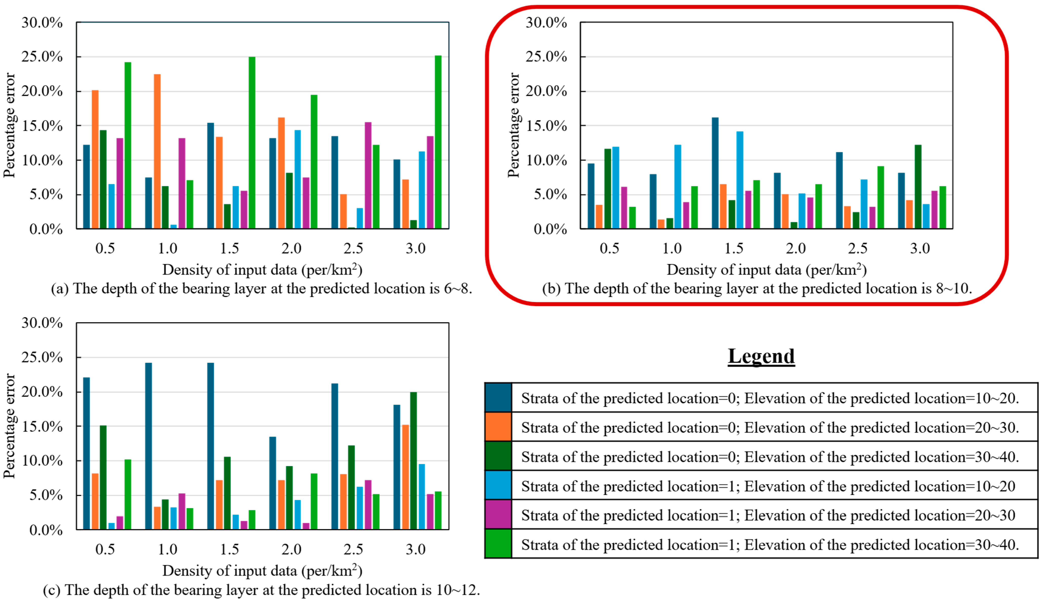
To ensure meaningful analysis, the evaluation was limited to data points within typical value ranges: bearing layer depth between 6 and 12 m, and elevation between 20 and 50 m. Predictions were then performed for each subset, and the results are shown in Figure 11. Prediction accuracy was assessed using percentage error (PE), defined by Equation (6):
P E = P r e d i c t e d   V a l u e A c t u a l   V a l u e A c t u a l   V a l u e × 100
A lower percentage error indicates higher prediction accuracy. To facilitate visual interpretation, color gradients were applied, with lighter shades representing lower error and hence better performance.
The results demonstrate that prediction accuracy improves with increasing data density, particularly when the bearing layer depth is in the range of 8 to 10 m. This suggests that spatially denser datasets enable the model to better capture local geotechnical variations, leading to more accurate predictions.
In general, complex machine learning models require more data to achieve stable and accurate predictions. As supported by prior studies [54,55], larger training datasets typically lead to better model generalization, with performance improvements often increasing logarithmically with data volume. The findings of this study support this trend, confirming the robustness and high potential of the random forest algorithm for geological prediction tasks.
However, the RF model is not without limitations. A key concern is overfitting, where the model performs well on training data but fails to generalize to unseen samples. Since random forests achieve flexibility by combining multiple deep decision trees, they may capture noise as signal in high-density scenarios. Therefore, mitigating overfitting is an important avenue for future research.
Two directions are proposed for improvement:
(1)
Integrating regularization techniques within the RF framework to reduce overfitting while maintaining predictive performance.
(2)
Exploring alternative machine learning algorithms and conducting comparative evaluations to identify models with superior generalization under varying geological conditions.
In addition, the training and testing data in this study are from the Tokyo region of Japan, which has a strong regional focus. Cross-regional cross-validation has not been performed under the current research framework, and the spatial generalization ability of the model still needs to be further explored. The significant differences in stratigraphic structure, and in water table and soil properties’ distribution in different regions may lead to unstable model migration effects. In the future, datasets from other regions (e.g., Kansai or Chubu region in Japan) will be introduced in the follow-up work, and attempts will be made to incorporate migration learning, regional adaptive modeling, and other methods to improve the applicability and robustness of the model in a wider geological context.

5.3. Practical Applications

The prediction model proposed in this study shows strong potential for practical applications. A promising future direction is to integrate it into geotechnical mapping tools based on geographic information systems (GIS), thereby enabling prediction of the spatial distribution of bearing layer depth over a wide area. In addition, the model can be deployed on a web-based platform to provide engineers and planners with preliminary remote estimates of subsurface conditions, potentially reducing the need for extensive field surveys in the early planning stages.
In addition, the model has potential applications in disaster risk management. For example, it can be integrated into hazard assessment frameworks to identify geotechnically vulnerable areas, such as those prone to liquefaction in earthquake-prone areas. These insights may help infrastructure planning and early warning strategies. Although these applications are currently at a conceptual stage, they represent important directions for future research and development.
Currently, most practical applications are still limited to the visualization of discrete measurement points on geospatial maps. Based on the results of this study, future work will focus on the development of a comprehensive software platform that can perform real-time subsurface predictions, update the output results to a central database, and integrate dynamic environmental indicators such as soil erosion or groundwater contamination.
Widespread access to detailed geotechnical information through smart digital tools has great potential to overcome the urban development challenges posed by subsurface uncertainty. Ultimately, this research can not only support safer and more resilient infrastructure but also promote more sustainable urban planning and improve the quality of life in growing cities.

6. Conclusions

This study evaluated and compared the predictive performance of three machine learning algorithms, random forest (RF), support vector machines (SVMs), and artificial neural networks (ANNs), for estimating bearing layer depth based on geotechnical data. Among the models tested, the random forest algorithm consistently outperformed the others in terms of accuracy and robustness, demonstrating its suitability for geological prediction tasks. The main findings are summarized as follows:
(1)
Feature-Based Prediction: The depth of the bearing layer can be effectively predicted using a combination of explanatory variables including latitude, longitude, elevation, and stratigraphic classification. The inclusion of a greater number of relevant features improves prediction accuracy, emphasizing the importance of comprehensive input data.
(2)
Model Performance and Data Density: Compared to SVM and ANN models, the RF model achieved superior performance. Furthermore, increasing the spatial density of training data significantly improved model accuracy. This highlights the importance of large-scale data collection for generating reliable geospatial predictions. The more extensive the dataset, the more detailed and accurate the resulting geotechnical maps.
Despite the encouraging results, this study has some important limitations that should be acknowledged and addressed in future research:
(1)
Limited external generalization: The model was trained and validated using data from a specific sub-region of the Tokyo metropolitan area. Therefore, its predictive reliability in geologically complex or remote areas remains uncertain. This geographic dependence limits the model’s generalization to wider applications without further validation.
(2)
Dependence on local stratigraphy: The model’s performance is related to the stratigraphic classification specific to the study area. Its applicability in different stratigraphic contexts may require retraining or adjustment, which may affect its robustness.
(3)
Model interpretability and credibility: While machine learning methods can achieve high prediction accuracy, their “black box” nature poses challenges to interpretability and credibility for safety-critical applications such as foundation design.
(4)
Missing potentially important explanatory variables: The current model does not consider variables such as groundwater level, distance to aquifers, or subsurface material properties. These factors may significantly affect prediction accuracy and should be incorporated into future work.
To overcome these limitations and improve model performance, future research will focus on the following directions:
(1)
Using advanced machine learning algorithms: Algorithms such as Nu-SVM, fuzzy and fractional-order SVM, rotation forests, and oblique random forests provide greater flexibility and robustness in terms of modeling complex non-linear relationships. The applicability of these methods to geotechnical datasets will be evaluated in future work.
(2)
Implementation of ensemble learning techniques: In addition to single models, we will further investigate ensemble learning strategies (e.g., majority voting, weighted averaging, and stacking) to combine the outputs of multiple algorithms. These approaches have the potential to integrate the strengths of different models and improve overall performance. Preliminary work has been initiated, and future studies will conduct a comprehensive evaluation of the ensemble effect.
By addressing these issues, we aim to build a more robust, general, and interpretable data-driven subsurface characterization framework.

Author Contributions

Conceptualization, S.I.; methodology, A.K.; software, Y.C. and A.K.; validation, A.K. and S.I.; formal analysis, Y.C. and A.K.; investigation, Y.C. and A.K.; resources, S.I.; data curation, Y.C. and A.K.; writing—original draft preparation, Y.C.; writing—review and editing, S.I.; visualization, Y.C. and A.K.; supervision, S.I.; project administration, S.I.; and funding acquisition, S.I. All authors have read and agreed to the published version of the manuscript.

Funding

This research received no external funding.

Data Availability Statement

The data that support the findings of this study are available from the corresponding author, Shinya Inazumi, upon reasonable request.

Conflicts of Interest

The authors declare no conflicts of interest.

References

  1. Seed, H.B.; Idriss, I.M. Simplified procedure for evaluating soil liquefaction potential. J. Soil Mech. Found. Div. 1971, 97, 1249–1273. [Google Scholar] [CrossRef]
  2. Seed, H.B.; Idriss, I.M. Ground Motions and Soil Liquefaction During Earthquakes; Earthquake Engineering Research Institute: Oakland, CA, USA, 1982; Volume 13, p. 13. [Google Scholar]
  3. Iwasaki, T.; Tokida, K.; Tatsuoka, F.; Watanabe, S.; Yasuda, S.; Sato, H. Microzonation for soil liquefaction potential using simplified methods. In Proceedings of the 3rd International Conference on Microzonation, Seattle, WA, USA, 1–6 November 1982; Volume 3, pp. 1319–1330. [Google Scholar]
  4. Seed, H.B.; Tokimatsu, K.; Harder, L.F.; Chung, R.M. Influence of SPT procedures in soil liquefaction resistance evaluation. J. Geotech. Eng. Div. 1985, 111, 1425–1445. [Google Scholar] [CrossRef]
  5. Liao, S.S.; Veneziano, D.; Whitman, R.V. Regression models for evaluating liquefaction probability. J. Geotech. Eng. 1988, 114, 389–411. [Google Scholar] [CrossRef]
  6. Matsuoka, M.; Wakamatsu, K.; Hashimoto, M.; Senna, S.; Midorikawa, S. Evaluation of liquefaction potential for large areas based on geomorphologic classification. Earthq. Spectra 2015, 31, 4. [Google Scholar] [CrossRef]
  7. Mohamed, W.; Radwa, E.; Mustafa, E.R.; Nassir, A.A.; Fathy, A.; Wael, M.E. Forecasting of flash flood susceptibility mapping using random forest regression model and geographic information systems. Heliyon 2024, 10, e33982. [Google Scholar] [CrossRef] [PubMed]
  8. Dou, J.; Hiromitsu, Y.; Hamid, R.P.; Ali, P.Y.; Song, X.; Xu, Y.; Zhu, Z. An integrated artificial neural network model for the landslide susceptibility assessment of Osado Island, Japan. Nat. Hazards 2015, 78, 1749–1776. [Google Scholar] [CrossRef]
  9. Hastie, T.; Tibshirani, R.; Friedman, J. Linear methods for classification. In The Elements of Statistical Learning, 2nd ed.; Springer: New York, NY, USA, 2009; pp. 101–137. [Google Scholar]
  10. Breiman, L.; Friedman, J.; Stone, C.J.; Olshen, R.A. Classification and Regression Trees; Chapman and Hall/CRC: Belmont, CA, USA, 1984; p. 368. [Google Scholar] [CrossRef]
  11. Porwal, A.; Carranza, E.J.M.; Hale, M. Artificial neural networks for mineral-potential mapping: A case study from Aravalli Province, Western India. Nat. Resour. Res. 2003, 12, 155–171. [Google Scholar] [CrossRef]
  12. Abedi, M.; Norouzi, G.H.; Bahroudi, A. Support vector machine for multi-classification of mineral prospectivity areas. Comput. Geosci. 2012, 46, 272–283. [Google Scholar] [CrossRef]
  13. Rodriguez-Galiano, V.F.; Chica-Olmo, M.; Chica-Rivas, M. Predictive modelling of gold potential with the integration of multisource information based on random forest: A case study on the Rodalquilar area, Southern Spain. Int. J. Geogr. Inf. Sci. 2014, 28, 1336–1354. [Google Scholar] [CrossRef]
  14. Rodriguez-Galiano, V.; Sanchez-Castillo, M.; Chica-Olmo, M.; Chica-Rivas, M. Machine learning predictive models for mineral prospectivity: An evaluation of neural networks, random forest, regression trees and support vector machines. Ore Geol. Rev. 2015, 71, 804–818. [Google Scholar] [CrossRef]
  15. Ren, X.; Hou, J.; Song, S.; Liu, Y.; Chen, D.; Wang, X.; Dou, L. Lithology identification using well logs: A method by integrating artificial neural networks and sedimentary patterns. J. Pet. Sci. Eng. 2019, 182, 106336. [Google Scholar] [CrossRef]
  16. Mienye, I.D.; Sun, Y. A survey of ensemble learning: Concepts, algorithms, applications, and prospects. IEEE Access 2022, 10, 99129–99149. [Google Scholar] [CrossRef]
  17. Yang, P.; Yang, Y.H.; Zhou, B.B.; Zomaya, A.Y. A review of ensemble methods in bioinformatics. Curr. Bioinform. 2022, 5, 296–308. [Google Scholar] [CrossRef]
  18. Sun, J.; Li, Q.; Chen, M.; Ren, L.; Huang, G.; Li, C.; Zhang, Z. Optimization of models for a rapid identification of lithology while drilling—A win-win strategy based on machine learning. J. Pet. Sci. Eng. 2019, 176, 321–341. [Google Scholar] [CrossRef]
  19. Xie, Y.; Zhu, C.; Zhou, W.; Li, Z.; Liu, X.; Tu, M. Evaluation of machine learning methods for formation lithology identification: A comparison of tuning processes and model performances. J. Pet. Sci. Eng. 2017, 160, 182–193. [Google Scholar] [CrossRef]
  20. Binh, T.P.; DieuTien, B.; Indra, P.; Dholakia, M.B. Evaluation of predictive ability of support vector machines and naive Bayes trees methods for spatial prediction of landslides in Uttarakhand State (India) using GIS. J. Geomat. 2016, 10, 71–79. [Google Scholar]
  21. Pakawan, C.; Saowanee, W. Predicting urban expansion and urban land use changes in Nakhon Ratchasima City using a CA-Markov model under two different scenarios. Land 2019, 8, 140. [Google Scholar] [CrossRef]
  22. Cong, Y.; Inazumi, S. Artificial neural networks and ensemble learning for enhanced liquefaction prediction in smart cities. Smart Cities 2024, 7, 2910–2924. [Google Scholar] [CrossRef]
  23. Matthias, S.; Rosie, Y.Z. The random forest algorithm for statistical learning. Stata J. 2020, 20, 3–29. [Google Scholar] [CrossRef]
  24. Cracknell, M.J.; Reading, A.M.; McNeill, A.W. Mapping geology and volcanic-hosted massive sulfide alteration in the Hellyer-Mt Charter region, Tasmania, using random forests and self-organising maps. Aust. J. Earth Sci. 2014, 61, 287–304. [Google Scholar] [CrossRef]
  25. Kuhn, S.; Cracknell, M.J.; Reading, A.M. Lithological mapping in the Central African Copper Belt using random forests and clustering: Strategies for optimised results. Ore Geol. Rev. 2019, 112, 103015. [Google Scholar] [CrossRef]
  26. Kuhn, S.; Cracknell, M.J.; Reading, A.M.; Sykora, S. Identification of intrusive lithologies in volcanic terrains in British Columbia by machine learning using random forests: The value of using a soft classifier. Geophysics 2020, 85, B235–B244. [Google Scholar] [CrossRef]
  27. Timothy, C.C.L.; Daniel, D.G.; Marek, A.; Well-Shen, L.; Sharon, A.C. Applying machine learning methods to predict geology using soil sample geochemistry. Appl. Comput. Geosci. 2022, 16, 100094. [Google Scholar] [CrossRef]
  28. Cong, Y.; Inazumi, S. Integration of smart city technologies with advanced predictive analytics for geotechnical investigations. Smart Cities 2024, 7, 1089–1108. [Google Scholar] [CrossRef]
  29. Cong, Y.; Inazumi, S. Ensemble learning for predicting subsurface bearing layer depths in Tokyo. Results Eng. 2024, 23, 102654. [Google Scholar] [CrossRef]
  30. Armaghani, D.J.; Asteris, P.G.; Mahmood, W.; Ghafor, K. Modeling flexural and compressive strengths behaviour of cement-grouted sands modified with water reducer polymer. Appl. Sci. 2022, 12, 1016. [Google Scholar] [CrossRef]
  31. Mahmood, W.; Mohammed, A.S.; Asteris, P.G.; Ghafor, W.; Ahmed, H. Interpreting the experimental results of compressive strength of hand-mixed cement-grouted sands using various mathematical approaches. Arch. Civ. Mech. Eng. 2022, 22, 19. [Google Scholar] [CrossRef]
  32. Shooshpasha, I.; Kordnaeij, A.; Dikmen, U.; MolaAbasi, H.; Amir, I. Shear wave velocity by support vector machine based on geotechnical soil properties. Nat. Hazards Earth Syst. Sci. Discuss. 2014, 2, 2443–2461. [Google Scholar] [CrossRef]
  33. Bagińska, M.; Srokosz, P.E. The optimal ANN model for predicting bearing capacity of shallow foundations trained on scarce data. arXiv 2018, arXiv:1810.08649. [Google Scholar] [CrossRef]
  34. Salem, S.; Ezzat, S.; El-Shafie, A. Hybrid ELM and MARS-based prediction model for bearing capacity of shallow foundations. Processes 2022, 10, 1013. [Google Scholar] [CrossRef]
  35. Kasama, K.; Whittle, A.J. Bearing capacity of spatially random cohesive soil using numerical limit analyses. J. Geotech. Geoenviron. Eng. 2011, 137, 989–996. [Google Scholar] [CrossRef]
  36. Al-Bittar, T.; Soubra, A.H. Bearing capacity of strip footings on spatially random soils using sparse polynomial chaos expansion. Int. J. Numer. Anal. Methods Geomech. 2013, 37, 2039–2060. [Google Scholar] [CrossRef]
  37. Jinhui, L.; Yinghui, T.; Mark, J.C. Failure mechanism and bearing capacity of footings buried at various depths in spatially random soil. J. Geotech. Geoenviron. Eng. 2014, 141, 2. [Google Scholar] [CrossRef]
  38. Bowles, J.E. Foundation Analysis, 3rd ed.; McGraw-Hill: New York, NY, USA, 2001. [Google Scholar]
  39. Yusof, N.Q.A.M.; Zabidi, H. Reliability of using standard penetration test (SPT) in predicting properties of soil. J. Phys. Conf. Ser. 2018, 1082, 012094. [Google Scholar] [CrossRef]
  40. Shan, S.; Pei, X.; Zhan, W. Estimating deformation modulus and bearing capacity of deep soils from dynamic penetration test. Adv. Civ. Eng. 2021, 2021, 1082050. [Google Scholar] [CrossRef]
  41. Katsuumi, A.; Cong, Y.; Inazumi, S. AI-driven prediction and mapping of soil liquefaction risks for enhancing earthquake resilience in smart cities. Smart Cities 2024, 7, 1836–1856. [Google Scholar] [CrossRef]
  42. Peter, B.; Bin, Y. Analyzing bagging. Ann. Stat. 2002, 30, 927–961. [Google Scholar] [CrossRef]
  43. Breiman, L. Bagging predictors. Mach. Learn. 1996, 24, 123–140. [Google Scholar] [CrossRef]
  44. Breiman, L. Random forests. Mach. Learn. 2001, 45, 5–32. [Google Scholar] [CrossRef]
  45. Gérard, B.; Erwan, S. A random forest guided tour. Test 2016, 25, 197–227. [Google Scholar]
  46. Hastie, T.; Tibshirani, R.; Friedman, J.H. The Elements of Statistical Learning: Data Mining, Inference and Prediction, 2nd ed.; Springer: New York, NY, USA, 2009; p. 533. [Google Scholar]
  47. Kotsiantis, S.B. Supervised machine learning: A review of classification techniques. Informatica 2007, 31, 249–268. [Google Scholar]
  48. Matthew, J.C.; Anya, M.R. Geological mapping using remote sensing data: A comparison of five machine learning algorithms, their response to variations in the spatial distribution of training data and the use of explicit spatial information. Comput. Geosci. 2014, 63, 22–33. [Google Scholar] [CrossRef]
  49. Vapnik, V.N. Statistical Learning Theory; John Wiley & Sons, Inc.: New York, NY, USA, 1998; p. 736. [Google Scholar]
  50. Karatzoglou, A.; Meyer, D.; Hornik, K. Support vector machines in R. J. Stat. Softw. 2006, 15, 1–28. [Google Scholar] [CrossRef]
  51. Jović, A.; Brkić, K.; Bogunović, N. A review of feature selection methods with applications. In Proceedings of the 38th International Convention on Information and Communication Technology, Electronics and Microelectronics (MIPRO), Opatija, Croatia, 25–29 May 2015; IEEE: New York, NY, USA, 2015. [Google Scholar]
  52. Sanjaya, K.P.; Prasanta, K.J. Efficient task scheduling algorithms for heterogeneous multi-cloud environment. J. Supercomput. 2015, 71, 1505–1533. [Google Scholar] [CrossRef]
  53. Patro, S.G.K.; Sahu, K.K. Normalization: A preprocessing stage. arXiv 2015, arXiv:1503.06462. [Google Scholar] [CrossRef]
  54. Alexander, K.; Lucas, B.; Xiaohua, Z.; Joan, P.; Jessica, Y.; Sylvain, G.; Neil, H. Big transfer (BiT): General visual representation learning. Comput. Vis.—ECCV 2020, 491, 491–507. [Google Scholar] [CrossRef]
  55. Chen, S.; Abhinav, S.; Saurabh, S.; Abhinav, G. Revisiting unreasonable effectiveness of data in deep learning era. In Proceedings of the IEEE International Conference on Computer Vision (ICCV), Venice, Italy, 22–29 October 2017; IEEE: New York, NY, USA, 2017; pp. 843–852. [Google Scholar] [CrossRef]
Figure 1. Schematic of bearing layer in relation to subsurface strata.
Make 07 00069 g001
Figure 2. Microtopographic classification map of southwestern Tokyo (Tokyo Geographical Research Institute).
Make 07 00069 g002
Figure 3. Geographic distribution of the 942 geotechnical survey points.
Make 07 00069 g003
Figure 4. Random forest architecture.
Make 07 00069 g004
Figure 5. Neural network architecture (PyTorch version 2.2.0).
Make 07 00069 g005
Figure 6. Support vector machine (SVM) conceptual structure.
Make 07 00069 g006
Figure 7. Prediction accuracy of Case-1 (latitude, longitude, and elevation only).
Make 07 00069 g007
Figure 8. Prediction accuracy of Case-2 (with stratigraphic classification).
Make 07 00069 g008
Figure 9. Training loss and validation loss curves of ANN in 500 rounds of training.
Make 07 00069 g009
Figure 10. Data subsets used for evaluating data density impact.
Make 07 00069 g010
Figure 11. Effect of data density on RF model prediction accuracy across six test cases.
Make 07 00069 g011
Table 1. Comparative analysis of predictive models for the depth of the holding layer or subsoil layer in different studies.
Authors and YearModel TypeInput FeaturesStudy AreaAccuracy Metrics
Salem et al. [32]DNN (ANN)Geometry, Soil propertiesShallow foundations (global)RMSE reduced by 12–17%
Rezaei et al. [33]SVMVs, SPT N value, CPT dataGeotechnical sitesComparable to direct test accuracy
Lin et al. [34]ML surveySPT N value, CPTu, Site featuresDisaster early-warning systemsDemonstrated efficacy
This studyRF, SVM, ANNLatitude, Longitude, Elevation, Stratigraphic classification, SPT N valueTokyo, Japan-
Table 2. Examples of input variables and bearing layer depth from three Tokyo sites.
Explanatory VariablesTarget Variable
LatitudeLongitudeStratigraphic classification *Elevation (m)Bearing layer depth (m)
35.64813984139.6406028035.16.2
35.64244679139.6641675031.05.8
35.64254438139.6479903137.710.0
* Diluvial layer = 1 and alluvial layer = 0.
Table 3. Optimized hyperparameters for the random forest model.
HyperparameterValue
n_estimators91
max_depthNone
oob_scoreTrue
bootstrapTrue
max_features5
Table 4. Configuration and training parameters of the artificial neural network (ANN) model.
ComponentDescription
Input features5
OutputBearing layer depth
Hidden layers3 layers (256 → 128 → 64 neurons)
Activation functionReLU
Loss functionMean Squared Error
Epochs500 and 1000
Table 5. Configuration and hyperparameters of the support vector machine (SVM) model.
ParameterDescriptionFinal Value
Kernel5RBF
CBearing layer depth1
Gamma (γ)3 layers (256 → 128 → 64 neurons)0.3
Cross-validationReLU10-fold
Feature ScalingMean Squared ErrorMin–Max
Table 6. Comparative prediction performance of RF, ANN, and SVM models (Cases-1 and -2).
Case-1Case-2
MAEMSERMSEMAEMSERMSE
RF1.263.061.750.861.141.07
ANNs1.587.012.651.072.891.7
SVMs1.714.532.131.272.531.59
Table 7. Model prediction comparison at three selected locations.
Point 1Point 2Point 3
Measured value (m)6.25.810
Predicted value (m)5.96.28.4
Disclaimer/Publisher’s Note: The statements, opinions and data contained in all publications are solely those of the individual author(s) and contributor(s) and not of MDPI and/or the editor(s). MDPI and/or the editor(s) disclaim responsibility for any injury to people or property resulting from any ideas, methods, instructions or products referred to in the content.

