AI-Driven Intelligent Financial Forecasting: A Comparative Study of Advanced Deep Learning Models for Long-Term Stock Market Prediction

Abstract

The integration of artificial intelligence (AI) and advanced deep learning techniques is reshaping intelligent financial forecasting and decision-support systems. This study presents a comprehensive comparative analysis of advanced deep learning models, including state-of-the-art transformer architectures and established non-transformer approaches, for long-term stock market index prediction. Utilizing historical data from major global indices (S&P 500, NASDAQ, and Hang Seng), we evaluate ten models across multiple forecasting horizons. A dual-metric evaluation framework is employed, combining traditional predictive accuracy metrics with critical financial performance indicators such as returns, volatility, maximum drawdown, and the Sharpe ratio. Statistical validation through the Mann–Whitney U test ensures robust differentiation in model performance. The results highlight that model effectiveness varies significantly with forecasting horizons and market conditions—where transformer-based models like PatchTST excel in short-term forecasts, while simpler architectures demonstrate greater stability over extended periods. This research offers actionable insights for the development of AI-driven intelligent financial forecasting systems, enhancing risk-aware investment strategies and supporting practical applications in FinTech and smart financial analytics.

1. Introduction

The increasing complexity of financial markets has driven substantial interest in advanced predictive analytics, with daily trading volumes reaching billions of dollars [1]. While various studies have demonstrated profitable predictive models [2,3], consistently outperforming the market remains challenging under the efficient market hypothesis [4]. The current literature reveals several critical gaps in financial time-series forecasting. Traditional forecasting methods struggle with capturing non-linear patterns and long-term dependencies in financial data [5], and although deep learning approaches have shown promise through their ability to handle large datasets and complex relationships [6], most studies have focused on short-term predictions, leaving long-term forecasting relatively underexplored.

The emergence of transformer-based architectures [7] has introduced new possibilities for addressing long-term dependencies, yet their application to financial forecasting presents unique challenges. Recent work by [8] questions the effectiveness of transformers in time-series forecasting, suggesting that simpler linear models might perform better in certain scenarios. This view contrasts with the findings in [9,10], which demonstrated successful applications of transformer models in financial markets—highlighting the need for a comprehensive comparative analysis. Furthermore, most studies rely solely on accuracy metrics, often overlooking crucial financial performance indicators. Ref. [11] highlight that the non-stationary nature of financial time series can lead to information loss during data preprocessing (a challenge termed “over-stationarization”). Non-stationarity refers to time series whose statistical properties, like mean and variance, change over time. In financial markets, non-stationarity appears as shifting trends, changing volatility, and structural breaks over time. These dynamics introduce distribution shifts and dependencies on exogenous factors, which can severely degrade predictive performance if not properly accounted for. Ref. [12] found that conventional approaches fail to capture the multi-periodic structures and complex interdependencies inherent in financial markets. Although innovative architectures have been introduced (e.g., [13,14], these evaluations are typically limited to specific time scales and market conditions, underscoring the need for a more comprehensive evaluation framework.

Recent surveys have further illuminated these challenges and opportunities. Ref. [15] reviewed the evolution of time series forecasting from traditional methods to diverse deep learning architectures, highlighting a recent shift toward architectural variety. Specifically, Ref. [16] provided an extensive review of transformer-based time-series forecasting, highlighting their ability to model long-term dependencies and identify potential pitfalls. These surveys not only consolidate current advancements but also reinforce the critical need for our comprehensive analysis.

This paper addresses these limitations through two primary research questions. First, we examine the strong empirical performance achievable by state-of-the-art transformer-based deep learning models in long-term stock market index forecasting. Second, we investigate which evaluation metrics and methodologies most effectively identify and validate superior-performing models in this context. Our work makes several distinct contributions. We provide the first comprehensive evaluation of ten models—encompassing both transformer-based and traditional architectures—across multiple forecasting horizons using data from three major global indices. Unlike previous studies that focus on specific market conditions, our analysis spans different market regimes and economic cycles. We employ a rigorous statistical testing framework through the Mann–Whitney U test, addressing the lack of statistical validation in comparative studies. Additionally, we introduce a multi-metric evaluation approach that combines traditional accuracy measures with financial performance indicators, offering a more complete assessment of model effectiveness.

The remainder of this paper is organized as follows: Section 2 presents a literature review and identifies current research gaps. Section 3 details our methodology, including data preprocessing, model architectures, and evaluation framework. Section 4 presents our empirical results and discussion, while Section 5 concludes with key findings and directions for future research.

2. Related Work

Financial time-series forecasting has evolved substantially through various methodological approaches, each contributing unique insights to the field. This review analyzes the key thematic developments that have shaped our understanding of market prediction. Traditional forecasting methods initially relied on fundamental and technical analysis approaches. Ref. [17] established the distinction between fundamental analysis, which evaluates corporate and macroeconomic data, and technical analysis, which focuses on historical price patterns. Early machine learning applications demonstrated promise, with [18] pioneering the integration of data mining and neural networks. Refs. [2,3] further advanced this direction through hybrid genetic–neural architectures and neuro-fuzzy methodologies, respectively.

The emergence of deep learning marked a transformative period in financial forecasting. Ref. [19] documented how deep neural networks revolutionized pattern recognition through automatic feature learning. Ref. [6] later synthesized these advances, demonstrating deep learning’s superior ability to handle large datasets and capture complex market relationships. This capability proved particularly valuable in stock market prediction, as evidenced by [20], which successfully integrated diverse data sources for market movement prediction. Recurrent neural architectures represented a significant advancement in handling sequential financial data. Ref. [21] demonstrated that LSTM networks are effective in addressing the vanishing gradient problem inherent in traditional RNNs. This work was extended by [22,23], which applied sophisticated time-series analysis techniques to stock price prediction. Ref. [24] enhanced these approaches by integrating principal component analysis with recurrent networks. Hybrid architectures emerged as a powerful approach to combining different modeling strengths. Ref. [25] integrated multiple CNN pipelines with BI-LSTM for enhanced temporal pattern analysis, while [26] explored combinations of LSTM, GRU, and ICA. Refs. [27,28] demonstrated the effectiveness of CNN-LSTM combinations in capturing both spatial and temporal patterns. Refs. [29,30] further refined these hybrid approaches through attention mechanisms.

The transformer architecture, introduced by [7], revolutionized sequential data processing [10] successfully adapted transformers for stock market prediction, while [9,31] demonstrated their effectiveness in emerging markets. However, challenges in processing long sequences led to several architectural innovations. Ref. [13] developed Autoformer with its decomposition architecture, while [14] introduced Informer to address efficiency challenges in long sequence processing. Recent research has focused on addressing specific challenges in financial forecasting. Ref. [11] tackled the critical issue of non-stationarity through their Non-stationary Transformers framework. Ref. [32] proposed Crossformer to capture cross-dimensional dependencies, while [33] introduced PatchTST with novel patching techniques. The relationship between model complexity and performance has been scrutinized by [34,35], which demonstrated that simpler linear models could sometimes outperform more complex approaches. Market-specific applications have provided valuable insights into model performance across different contexts. Ref. [36] conducted a detailed analysis of S&P market indices, while [1] emphasized the importance of diverse variable sets in prediction accuracy. These applications have been complemented by methodological innovations, such as TimesNet [12] for handling multi-periodic patterns and FiLM [37] for balancing complexity with efficiency.

The current literature reveals several critical gaps. Despite numerous methodological advances, comprehensive comparative analyses across different market conditions and time horizons remain limited. Evaluation frameworks often emphasize technical accuracy over practical financial metrics, as noted in [4] in their review of machine learning applications in stock market forecasting. Additionally, the relationship between model complexity and forecasting reliability requires deeper investigation, particularly in the context of varying market conditions. Our research addresses these gaps through a comprehensive evaluation framework that spans multiple models, time horizons, and market conditions. By integrating both traditional accuracy metrics and financial performance indicators, we provide a more complete assessment of model effectiveness in practical applications. This approach allows us to contribute to the ongoing discussion about the optimal balance between model sophistication and practical utility in financial forecasting.

3. Methodology

This section presents our representative comparative framework for evaluating deep learning models in long-term stock market forecasting. Our methodology encompasses data acquisition and preprocessing, model architectures, experimental design, and evaluation metrics.

Data preparation forms the foundation of our analysis. We utilize daily closing price data from three major stock indices: S&P 500, NASDAQ, and Hang Seng Index (HSI), spanning from 24 November 1969, to 7 August 2023. Each dataset contains essential price indicators: opening price, highest price, lowest price, and closing price. We specifically excluded trading volume due to data completeness considerations. Following [11,13], we implement a standardization process to address the non-stationary characteristics inherent in financial time series. Our data preprocessing protocol involves several key steps. First, we clean the numerical values by removing commas and standardizing date formats. We employ the StandardScaler technique to normalize values within the range of −1 to 1, following practices established in [10]. The dataset was split into training, validation, and test sets using a 70:20:10 ratio while preserving temporal order. The test set corresponds to the most recent portion of the time series, ensuring no look-ahead bias or foresight effects in model evaluation.

We selected 10 transformer models that represent well the distinct architectural innovations within the time series forecasting landscape. For instance, Autoformer focuses on decomposition, Informer improves efficiency for long sequences, Crossformer captures cross-dimensional dependencies, Non-stationary Transformer adapts to time-varying structures, and PatchTST employs a novel patch-based learning mechanism. These models have demonstrated state-of-the-art performance in the prior literature, making them suitable benchmarks for this comparative study. In summary, the transformer models in our study include the original Transformer [7], Autoformer [13], Informer [14], Crossformer [32], Non-stationary Transformer [11], and PatchTST [33] models. The non-transformer models comprise TimeNet [12], MICN [38], FiLM [37], and Dlinear [8]. Our experiments were run on a virtualized environment hosted on a machine with an Intel Core i7-12700 CPU, 32GB RAM, and NVIDIA GeForce GTX 3070 GPU. The implementation is based on Python v3.11 with key libraries, including NumPy v1.23.5, Pandas v1.5.3, and Torch v1.7.1. Where applicable, we maintain consistent hyperparameter settings across models: 96-time step look-back window, input dimensions of 5, output dimension of 1, and 8 attention heads for transformer-based models. Each model is trained to perform direct multi-step forecasting across multiple horizons (96, 192, 336, and 720 days), meaning it predicts an entire future sequence in a single pass rather than through repeated one-day-ahead steps. While these horizons are long in terms of sequence length, we acknowledge that this setup more closely aligns with short-term trading evaluation than long-term investment modeling.

Training configurations include a batch size of 32, with mean squared error as the loss function. The model dimension is 512, and the feedforward network dimension is 2048, except for Autoformer and Crossformer, which use 64 dimensions. We employ the Adam optimizer with a learning rate of 0.0001 across 10 epochs, ensuring consistent training dynamics while preventing overfitting. For evaluation, we employ a dual-metric approach combining technical accuracy measures with financial performance indicators. Following [39], we utilize Mean Absolute Error (MAE) and Mean Squared Error (MSE) for accuracy assessment. Financial performance evaluation incorporates return calculation, volatility assessment, maximum drawdown analysis, and Sharpe ratio computation, following methodologies established in [10]. Our trading strategy is deliberately simplistic, using a threshold-based rule applied to each individual index independently to ensure that observed financial outcomes are primarily reflective of the model’s directional prediction capability. While this setup avoids cross-asset interference, we acknowledge that it may conflate suboptimal strategy design with model prediction quality. A long position is taken if the predicted next-day closing price exceeds the current day’s closing price; otherwise, the position is neutral. No short-selling was incorporated. Returns are calculated based on the change in actual price following this rule. This approach isolates the model’s forecasting quality from more complex trading heuristics, enabling a cleaner comparison. So, we implement a trading strategy where position decisions are based on predicted value movements:

$$R_{t+1}=ln(\frac{{\hat{x}}_{t+1}}{x_t})\times \mathrm{sign}({\hat{x}}_{t+1}-x_t)$$

where $x_t$ and ${\hat{x}}_{t+1}$ represent the actual closing price and the predicted price, respectively.

A long position is taken only if the predicted price exceeds the current price. Returns are adjusted by subtracting a transaction cost of 0.1%. The cumulative net value is computed by summing realized returns over the forecasting horizon.

The net value calculation considers transaction costs of 0.1%, reflecting real-world trading conditions:

$$NetValue=GrossValue-\sum _{i=1}^n{P}_{i}x r$$

where $P_i$ is the position value for the i-th trade, and r is the transaction cost rate (0.1%).

Our statistical validation is based on the two-sided Mann–Whitney U test to evaluate whether the forecasting errors (e.g., MSEs) from one model are statistically different in central tendency from those of another. This non-parametric test does not compare full distributions but tests whether the Hodges–Lehmann estimate of the difference in location between two samples is significantly different from zero. Our experimental protocol evaluates forecasting performance across multiple time horizons (96, 192, 336, and 720 days) to assess model reliability in different prediction scenarios. This comprehensive approach allows us to examine both short-term accuracy and long-term stability, addressing a significant gap in the existing literature identified by [9,31].

Our methodology provides a rigorous framework for comparing model performance while considering both technical accuracy and practical financial implications. The multi-metric evaluation approach, combined with statistical validation, ensures robust and meaningful comparisons across different model architectures and forecasting horizons.

4. Results and Discussion

In this section, we evaluate the performance of models in direct multi-step forecasting tasks across horizons of 96, 192, 336, and 720 days. Each model generates the full sequence of predictions in a single forward pass without recursive use of previous predictions. The results are thus interpreted as a measure of forecast accuracy and stability over long horizons rather than simulations of day-by-day predictive updates.

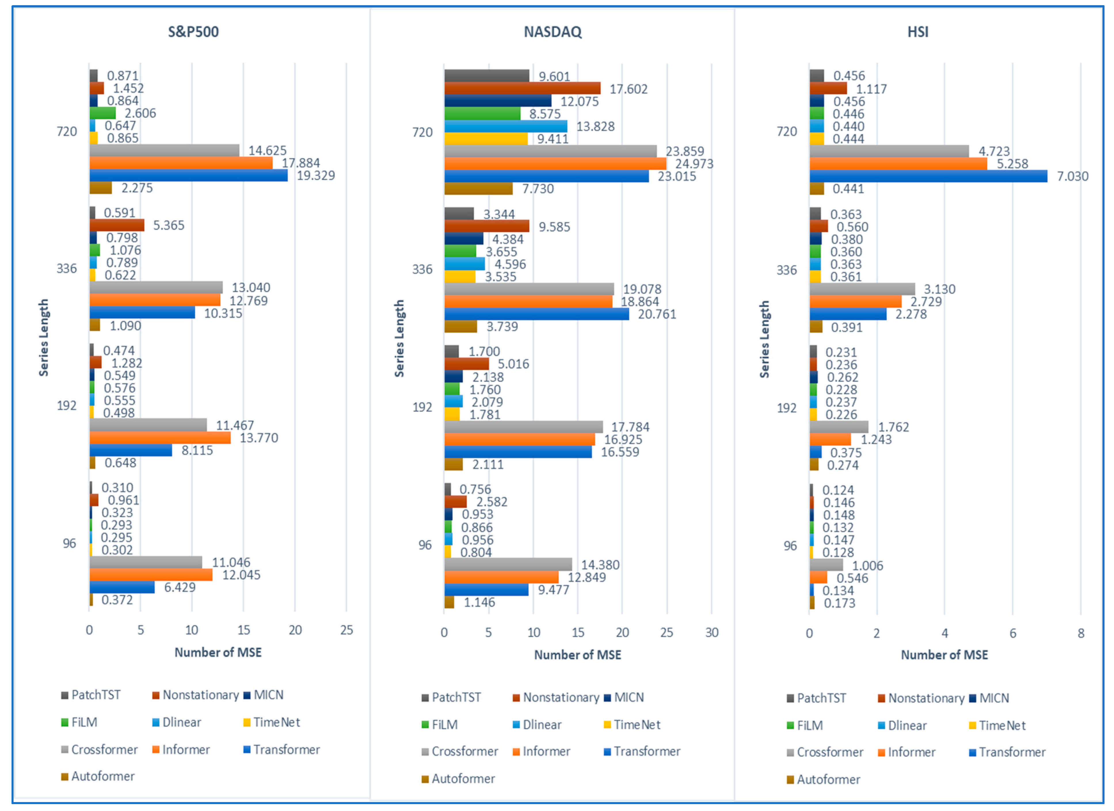
Based on our experiments and findings summarized and shown in Figure 1, we can see the overall comparison of MSE of ten models among three datasets. MSE values are calculated on standardized (z-score normalized) closing prices. By examining predictive accuracy across the S&P 500 dataset, the PatchTST model demonstrates superior performance for series lengths of 192 and 336 days, achieving the lowest MSE values among all models. For the shortest series length of 96 days, the FiLM model excels with an MSE of 0.293, while the Dlinear model achieves strong empirical performance for the extended 720-day horizon with an MSE of 0.647. These findings align with the observation in [8] that simpler architectures can outperform complex models in certain scenarios. The NASDAQ dataset analysis reinforces PatchTST’s effectiveness, showing consistent superior performance across the 96-, 192-, and 336-day forecasting horizons. This performance validates the assertion by [33] regarding the benefits of patch-based processing in capturing local temporal patterns. However, for the 720-day horizon, the Autoformer model demonstrates better accuracy, supporting the findings from [13] on the effectiveness of decomposition-based approaches for longer-term forecasting.

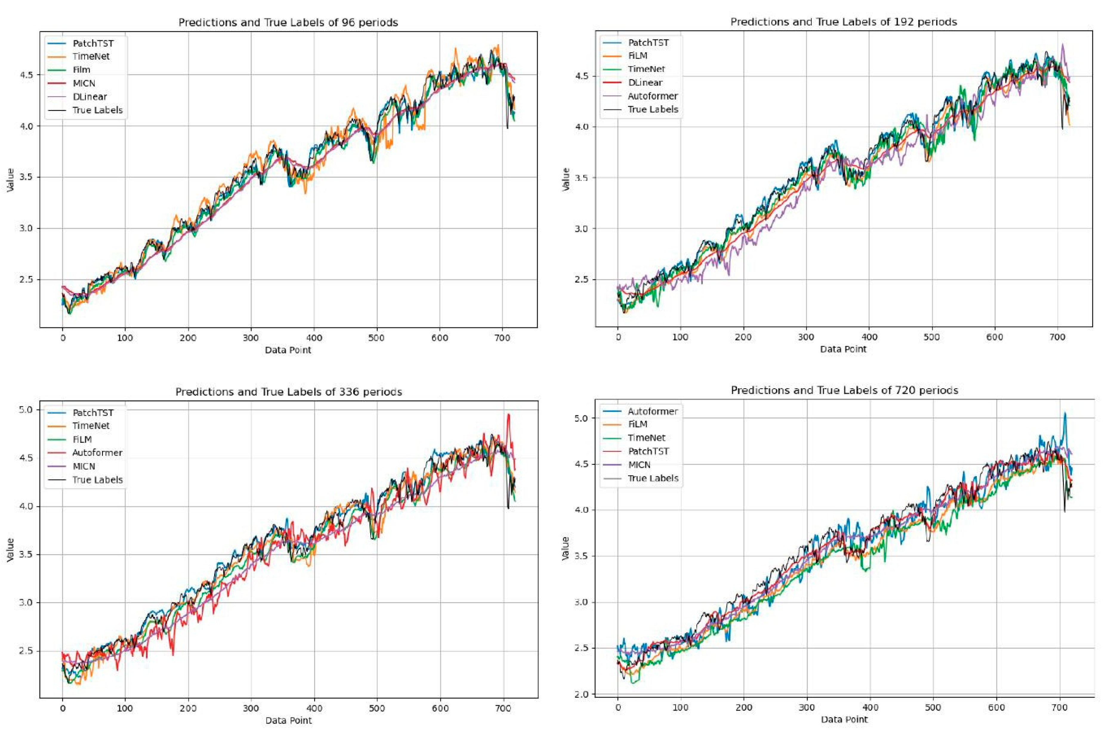
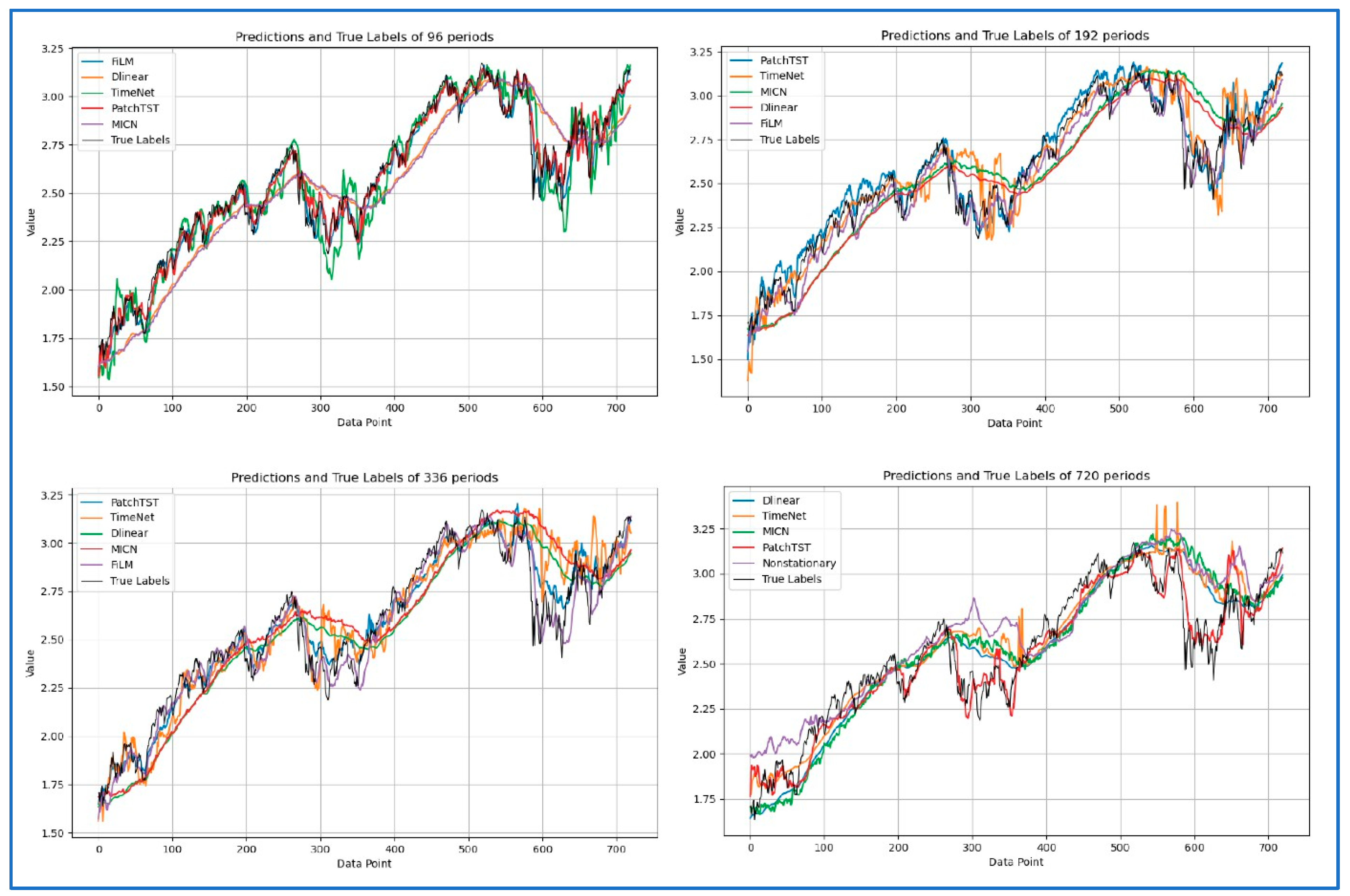
Results from the HSI dataset reveal a more nuanced pattern. PatchTST maintains its superiority for 96-day forecasting, while TimeNet excels in 192-day predictions. FiLM demonstrates exceptional performance during the 336-day interval, aligning with the findings from [37] on the effectiveness of frequency-enhanced architectures. Notably, Dlinear consistently achieves the lowest scores over 720-day periods, challenging the assumption that more complex architectures necessarily yield better results for extended forecasting horizons. We also demonstrate the results of the predictions and true labels using a look-back window of 96 with forecasting series lengths of 96, 192, 336, and 720 in the HIS, NASDAQ, and S&P500 datasets in Figure 2, Figure 3 and Figure 4, respectively. Five representative models were selected based on their performance to avoid visual clutter. Some models exhibit noticeable deviations at the beginning of the forecast horizon, particularly under long-range settings. This reflects a combination of sensitivity to sharp market changes and limitations in early-step calibration during multi-step prediction. These patterns reinforce the finding that model robustness varies significantly across architectures and time regimes. Model tuning was uniform across architectures to preserve fairness, which may have affected some models’ ability to generalize at short-term offsets.

From another perspective, financial performance metrics provide crucial insights into practical model utility.

Financial Metric. (1) Return: total percentage increase in portfolio value; (2) volatility: standard deviation of daily returns; (3) maximum drawdown (MaxDrawdown): the largest relative peak-to-trough loss observed in the cumulative return series over the forecasting period; and (4) Sharpe ratios are calculated using a risk-free rate of 0%, focusing on model-relative performance rather than real-world absolute returns.

Table 1. The average statistical performance across the models during a 96-day duration.

An Average of the Models’ Statistical Performance over a 96-Day Period
Models	Return (%)	Volatility (%)	MaxDrawdown(%)	Sharpe Ratio
Autoformer	9.13	6.53	79.32	0.806
Crossformer	49.89	29.52	77.07	1.608
Dlinear	8.19	6.25	81.59	0.687
Film	7.98	6.36	85.65	0.645
Informer	46.96	28.86	79.68	1.442
MICN	8.38	6.27	82.10	0.721
Nonstationary	11.42	9.79	83.40	0.764
PatchTST	7.27	6.43	86.30	0.529
TimeNet	7.16	6.59	87.33	0.493
Transformer	28.28	21.33	79.74	1.034

,

Table 2. The average statistical performance across the models during a 192-day duration.

An Average of the Models’ Statistical Performance over a 192-Day Period
Models	Return (%)	Volatility (%)	MaxDrawdown(%)	Sharpe Ratio
Autoformer	11.65	8.65	80.59	0.447
Crossformer	62.72	30.94	60.05	1.907
Dlinear	11.32	8.56	79.69	0.392
Film	10.79	8.72	81.37	0.353
Informer	63.74	34.09	68.92	1.666
MICN	11.43	8.65	80.69	0.390
Nonstationary	14.62	12.98	88.11	0.492
PatchTST	9.79	8.88	90.30	0.219
TimeNet	10.11	8.65	89.38	0.253
Transformer	44.42	28.41	75.39	1.206

,

Table 3. Average statistical performance across the models during a 336-day duration.

An average of the Models’ Statistical Performance over a 336-Day Period
Models	Return (%)	Volatility (%)	MaxDrawdown(%)	Sharpe Ratio
Autoformer	14.74	11.30	80.90	0.094
Crossformer	80.65	30.37	42.44	2.412
Dlinear	15.01	11.60	79.00	−0.004
Film	14.43	11.87	79.29	0.069
Informer	75.70	38.60	61.10	1.824
MICN	14.78	11.37	80.58	−0.002
Nonstationary	25.55	24.12	82.60	0.497
PatchTST	12.28	10.87	85.52	−0.263
TimeNet	12.85	10.67	87.36	−0.199
Transformer	71.27	46.42	73.59	1.300

and

Table 4. Average statistical performance across the models during a 720-day duration.

An Average of the Models’ Statistical Performance over a 720-Day Period
Models	Return (%)	Volatility (%)	MaxDrawdown(%)	Sharpe Ratio
Autoformer	20.98	14.72	80.23	−0.619
Crossformer	113.14	34.48	45.25	2.723
Dlinear	23.69	15.51	80.33	−0.988
Film	22.28	16.82	76.54	−0.472
Informer	125.69	65.46	56.40	1.699
MICN	22.52	15.08	80.36	−0.882
Nonstationary	31.09	23.53	81.75	−0.218
PatchTST	19.54	14.58	88.41	−1.032
TimeNet	19.61	13.77	88.43	−1.035
Transformer	139.63	72.81	67.04	1.559

summarize the average statistical performance across the models during 96-day, 192-day, 336-day, and 720-day durations, respectively. The Crossformer model demonstrates remarkable returns, achieving 49.89% and 46.96% for 96-day forecasting, though with relatively high volatility (29.52%) and a significant maximum drawdown (77.07%). This trade-off between return and risk aligns with Zhang and Yan’s (2022) [32] observations about the model’s characteristics. In contrast, models like Non-stationary and Autoformer exhibit more conservative profiles, offering lower returns but with reduced volatility and smaller drawdowns. For longer horizons (336 and 720 days), we observe increasing performance differentiation. Crossformer maintains strong performance with an average return of 80.65% over 336 days, rising to 113.14% over 720 days, albeit with elevated volatility levels of 30.37% and 34.48%, respectively. The Transformer model demonstrates comparable strength, achieving 71.27% returns over 336 days and 139.63% over 720 days, supporting C. Wang et al.’s (2022) [10] findings on transformer effectiveness in long-term forecasting. While these results suggest strong forecasting ability, we acknowledge that the performance may be partially influenced by the trading strategy employed. However, the use of the Mann–Whitney U test helps confirm that the observed differences stem from model outputs rather than trading rules alone. Future work could explore multiple trading strategies to better isolate the model’s intrinsic forecasting performance.

We also perform statistical validation through two-sided Mann–Whitney U tests, which reveal significant insights into model reliability. We define a null hypothesis (H₀) as follows: there is no significant difference in predictive performance between the two models under comparison. If p-value < 0.05, we reject H₀, indicating statistically significant differences. The analysis of p-values across different forecasting horizons reveals evolving model effectiveness, as shown in

Table 5. The p-value associated with the collection of MSE from a 96-day forecasting.

The p-Value of 96 Days
	Group2	Autoformer	Crossformer	Dlinear	Film	Informer	MICN	Nonstationary	PatchTST	TimeNet	Transformer
Group1
Autoformer			0.95	0.35	0.35	0.95	0.35	0.65	0.35	0.35	0.35
Crossformer		0.1		0.05	0.05	0.5	0.05	0.1	0.05	0.05	0.2
Dlinear		0.8	1		0.35	0.95	0.65	0.8	0.5	0.5	0.8
Film		0.8	1	0.8		0.95	0.8	0.9	0.5	0.5	0.9
Informer		0.1	0.65	0.1	0.1		0.1	0.2	0.1	0.1	0.2
MICN		0.8	1	0.5	0.35	0.95		0.8	0.35	0.35	0.8
Nonstationary		0.5	0.95	0.35	0.2	0.9	0.35		0.2	0.2	0.8
PatchTST		0.8	1	0.65	0.65	0.95	0.8	0.9		0.65	0.9
TimeNet		0.8	1	0.65	0.65	0.95	0.8	0.9	0.5		0.9
Transformer		0.35	0.9	0.35	0.2	0.9	0.35	0.35	0.2	0.2

,

Table 6. The p-value associated with the collection of MSE from a 192-day forecasting.

The p-Value of 192 Days
	Group2	Autoformer	Crossformer	Dlinear	Film	Informer	MICN	Nonstationary	PatchTST	TimeNet	Transformer
Group1
Autoformer			0.95	0.35	0.35	0.95	0.5	0.65	0.35	0.35	0.9
Crossformer		0.1		0.1	0.05	0.5	0.1	0.1	0.05	0.1	0.35
Dlinear		0.8	0.95		0.5	0.95	0.65	0.65	0.35	0.35	0.9
Film		0.8	1	0.65		0.95	0.65	0.8	0.5	0.5	0.9
Informer		0.1	0.65	0.1	0.1		0.1	0.2	0.1	0.1	0.35
MICN		0.65	0.95	0.5	0.5	0.95		0.65	0.35	0.35	0.9
Nonstationary		0.5	0.95	0.5	0.35	0.9	0.5		0.35	0.35	0.9
PatchTST		0.8	1	0.8	0.65	0.95	0.8	0.8		0.65	0.9
TimeNet		0.8	0.95	0.8	0.65	0.95	0.8	0.8	0.5		0.9
Transformer		0.2	0.8	0.2	0.2	0.8	0.2	0.2	0.2	0.2

,

Table 7. The p-value associated with the collection of MSE from a 336-day forecasting.

The p-Value of 336 Days
	Group2	Autoformer	Crossformer	Dlinear	Film	Informer	MICN	Nonstationary	PatchTST	TimeNet	Transformer
Group1
Autoformer			0.95	0.5	0.35	0.95	0.5	0.9	0.35	0.35	0.95
Crossformer		0.1		0.1	0.1	0.35	0.1	0.2	0.1	0.1	0.5
Dlinear		0.65	0.95		0.5	0.95	0.65	0.9	0.41	0.35	0.95
Film		0.8	0.95	0.65		0.95	0.65	0.9	0.5	0.5	0.95
Informer		0.1	0.8	0.1	0.1		0.1	0.2	0.1	0.1	0.5
MICN		0.65	0.95	0.5	0.5	0.95		0.9	0.35	0.35	0.95
Nonstationary		0.2	0.9	0.2	0.2	0.9	0.2		0.2	0.2	0.9
PatchTST		0.8	0.95	0.74	0.65	0.95	0.8	0.9		0.65	0.95
TimeNet		0.8	0.95	0.8	0.65	0.95	0.8	0.9	0.5		0.95
Transformer		0.1	0.65	0.1	0.1	0.65	0.1	0.2	0.1	0.1

and

Table 8. The p-value associated with the collection of MSE from a 720-day forecasting.

The p-value of 720 Days
	Group2	Autoformer	Crossformer	Dlinear	Film	Informer	MICN	Nonstationary	PatchTST	TimeNet	Transformer
Group1
Autoformer			0.95	0.5	0.8	0.95	0.65	0.65	0.65	0.65	0.95
Crossformer		0.1		0.1	0.1	0.8	0.1	0.2	0.1	0.1	0.65
Dlinear		0.65	0.95		0.65	0.95	0.65	0.9	0.65	0.65	0.95
Film		0.35	0.95	0.5		0.95	0.65	0.65	0.65	0.5	0.95
Informer		0.1	0.35	0.1	0.1		0.1	0.1	0.1	0.1	0.65
MICN		0.5	0.95	0.5	0.5	0.95		0.9	0.58	0.5	0.95
Nonstationary		0.5	0.9	0.2	0.5	0.95	0.2		0.2	0.2	0.95
PatchTST		0.5	0.95	0.5	0.5	0.95	0.58	0.9		0.35	0.95
TimeNet		0.5	0.95	0.5	0.65	0.95	0.65	0.9	0.8		0.95
Transformer		0.1	0.5	0.1	0.1	0.5	0.1	0.1	0.1	0.1

. PatchTST consistently achieves higher p-values across multiple comparisons, particularly for shorter forecasting horizons, indicating robust statistical significance in its performance advantages. For 96-day forecasting, PatchTST records strong evidence for the null hypothesis of superior performance. For 192-day and 336-day predictions, PatchTST maintains its statistical advantage. However, for 720-day predictions, TimeNet and Autoformer emerge as statistically superior performers, indicating a transition in model effectiveness over longer horizons.

In summary, our findings carry several important implications for both research and practice. First, they demonstrate that model selection should carefully consider the intended forecasting horizon, as performance characteristics vary significantly across different time scales. Second, they highlight the importance of balancing model complexity with practical considerations, supporting [11] about the trade-offs between model sophistication and practical utility. Our results also reveal a nuanced relationship between model architecture and market characteristics. The consistent performance of PatchTST across different markets suggests the effectiveness of its patch-based approach in capturing market dynamics, while the varying performance of other models indicates sensitivity to market-specific features. This observation aligns with the findings in [36] regarding the importance of market-specific considerations in model selection. Furthermore, our analysis suggests that traditional accuracy metrics alone may not fully capture model utility in practical applications, and the sometimes-divergent rankings between MSE/MAE metrics and financial performance indicators emphasize the importance of comprehensive evaluation frameworks, as suggested by [1].

5. Conclusions and Future Work

Our comprehensive evaluation of deep learning models for long-term stock market forecasting provides significant insights into the effectiveness of these models across various time horizons and market conditions. The PatchTST architecture demonstrates superior performance for shorter forecasting horizons in the S&P 500 and NASDAQ markets, validating the effectiveness of patch-based processing in capturing local temporal patterns. However, the Crossformer and Transformer models show more robust performance, albeit with increased volatility. Our analysis challenges conventional assumptions about model complexity, as simpler architectures, such as Dlinear, sometimes outperform more sophisticated models, particularly in longer horizons. The statistical validation through two-sided Mann–Whitney U tests provides robust evidence for horizon-specific model selection, while financial performance metrics reveal crucial insights into the practical utility of models beyond traditional accuracy measures. While this test is widely used, it assumes i.i.d. observations and does not control for multiple comparisons. To mitigate these limitations, our future work can adopt the Friedman test for global comparisons across multiple models, followed by non-parametric post hoc procedures (e.g., Nemenyi test) to identify significant pairwise differences. We acknowledge that drawdowns of 40–80% are high and reflect the limitations of the naive threshold-based trading strategy. In the future, we could apply rolling-window backtesting to offer greater robustness, as well as strategy-agnostic metrics (e.g., directional accuracy or classification AUC) or coupled model–strategy optimization to better decouple model quality from execution effects.