Article

Exploiting the Feature Space Structures of KNN and OPF Algorithms for Identification of Incipient Faults in Power Transformers

by
André Gifalli
1,*,
Marco Akio Ikeshoji
2,
Danilo Sinkiti Gastaldello
3,
Victor Hideki Saito Yamaguchi
1,
Welson Bassi
4,
Talita Mazon
5,
Floriano Torres Neto
1,
Pedro da Costa Junior
1 and
André Nunes de Souza
1
1
School of Engineering, São Paulo State University (UNESP), Bauru 17033-360, SP, Brazil
2
Federal Institute of Education, Science and Technology (IFSP), Birigui 16201-407, SP, Brazil
3
Faculty of Engineering, University of Marilia (UNIMAR), Marília 17525-902, SP, Brazil
4
High Voltage Laboratory, Institute of Energy and Environment (IEE), University of São Paulo (USP), São Paulo 05508-010, SP, Brazil
5
Micro and NanoMaterials Division, Renato Archer Information Technology Center, Campinas 13069-901, SP, Brazil
*
Author to whom correspondence should be addressed.
Mach. Learn. Knowl. Extr. 2025, 7(3), 102; https://doi.org/10.3390/make7030102
Submission received: 3 July 2025 / Revised: 25 August 2025 / Accepted: 8 September 2025 / Published: 18 September 2025

Abstract

Power transformers represent critical assets within the electrical power system, and their unexpected failures may result in substantial financial losses for both utilities and consumers. Dissolved Gas Analysis (DGA) is a well-established diagnostic method extensively employed to detect incipient faults in power transformers. Although several conventional and machine learning techniques have been applied to DGA, most of them focus only on fault classification and lack the capability to provide predictive scenarios that would enable proactive maintenance planning. In this context, the present study introduces a novel approach to DGA interpretation, which highlights the trends and progression of faults by exploring the feature space through the algorithms k-Nearest Neighbors (KNN) and Optimum-Path Forest (OPF). To improve accuracy, the following strategies were implemented: statistical filtering based on normal distribution to eliminate outliers from the dataset; augmentation of gas-related features; and feature selection using optimization algorithms such as Cuckoo Search and Genetic Algorithms. The approach was validated using data from several transformers, with fault diagnoses cross-checked against inspection reports provided by the utility company. The findings indicate that the proposed method offers valuable insights into the progression, proximity, and classification of faults with satisfactory accuracy, thereby supporting its recommendation as a complementary tool for diagnosing incipient transformer faults.

1. Introduction

Dissolved Gas Analysis (DGA) of insulating oils is a widely used technique for assessing the operational condition of power transformers [1]. It serves as a means of identifying potential incipient faults and subsequently guiding necessary actions, such as performing complementary verification tests or scheduling equipment inspection and maintenance.
The concentration of dissolved gases can be measured either through continuous gas monitoring devices installed on the transformer or by periodically extracting and analyzing samples with portable equipment on-site or in a laboratory, which is the most common procedure. In the latter case, the interval between analyses depends on the difference in gas concentrations measured in successive samples, since a sharp increase in gas levels over a short period strongly indicates the progression of an internal fault [2,3]. Under normal operating conditions, gases are typically analyzed once or twice per year; however, when a fault is suspected, the interval is shortened to months, weeks, or even days, depending on the severity of the condition.
The suspicion of a fault triggers the application of DGA interpretation techniques as a means of fault identification, which explains the availability of several conventional interpretation and diagnostic methods [4,5]. Although some of these techniques have been standardized, accurately diagnosing the fault type remains challenging, as they are often affected by gaps in fault classification criteria or by gas combinations that lead to inconsistent or ambiguous results. Consequently, no single method has achieved universal acceptance [6].
These inconsistencies arise from the non-linear behavior of dissolved gas generation in oil, which is influenced by thermal and electrical stresses, chemical reactions between materials, and other factors. Consequently, this has motivated research on various machine learning algorithms, aiming not only to enhance the success rate of conventional techniques but also to improve the accuracy of intelligent algorithms themselves by combining classifiers with optimization algorithms, statistical methods, and other approaches, as outlined below: Ref. [7] developed an Artificial Neural Network (ANN) for Pattern Recognition (PRN) to classify transformer operating conditions—normal, thermal, and electrical faults—based on combustible gases obtained from DGA. Using configurations with five and ten neurons in the hidden layer, the model achieved 98% overall accuracy on 815 real samples and 100% in validation, demonstrating its effectiveness as a diagnostic tool. Ref. [8] applied Multilayer Artificial Neural Network (ANN) and Support Vector Machine (SVM) models to predict transformer faults using Dissolved Gas Analysis (DGA) data. The ANN achieved a diagnostic accuracy of 76%, while the SVM achieved 81.4%, demonstrating that SVM outperformed ANN on the same dataset; Ref. [6] applied an ensemble of machine learning models, including random forest combined with scoring indices from conventional DGA ratios, demonstrating superior performance compared to standalone Extreme Learning Machine (ELM) approaches in transformer fault classification; Ref. [9] reviewed advanced feature extraction and dimensionality reduction methods, including PCA and kernel-based variants, applied to DGA data as input vectors for machine learning classifiers, demonstrating superior diagnostic accuracy compared to conventional gas ratio features; Ref. [10] proposed an interpretable machine learning framework based on edge inference for transformer DGA diagnosis, integrating feature extraction, optimization, and explainability to enhance classification accuracy in real-time; Ref. [11] proposed a causal reasoning approach for transformer fault diagnosis based on DGA. By integrating causality inference with conventional DGA frameworks and validating on 96 historical transformer samples, their method was able to diagnose all common transformer states, considering severity levels of thermal and electrical faults, achieving an overall accuracy of 95.8%; Ref. [12] employed SHAP for feature selection from DGA data and optimized a LightGBM classifier via Bald Eagle Search, demonstrating higher diagnostic accuracy than traditional feature selection approaches like Duval’s Pentagon; Ref. [13] introduced a feature-weighted domain adaptation technique combining MMD and CORAL to address distribution shifts in DGA datasets, significantly improving model generalization across transformers; Ref. [14] benchmarked traditional ML and DL models (including SVM, RF, XGBoost, LSTM, 1D-CNN) for DGA-based transformer fault detection, revealing comparable performance between RF and 1D-CNN with accuracy exceeding 86%, suggesting both approaches are viable; Other techniques were also discussed in [4].
In this manuscript, beyond the aforementioned techniques that merely identify specific fault types in transformers, we propose a novel gas interpretation analysis method. This approach leverages the graph structure of the feature space explored by the KNN and OPF classifiers, in association with historical data on fuel gases dissolved in insulating oil, to observe and diagnose the progression of incipient faults in transformers. Initially, datasets obtained from IEC TC10, IEEE Dataport, and related studies were pre-processed to eliminate outliers. Subsequently, gas data were combined to generate 17 types of features, which were evaluated using the Cuckoo Search (CS) and Genetic Algorithm (GA). The most relevant features were then selected to construct the training sets for KNN and OPF. Subsequently, the operational behavior of several transformers was evaluated, and the results were validated against inspection reports from the utility company. A clear coherence was observed between the evolution of dissolved gas behavior and the fault trends, thereby supporting the use of this technique as an additional diagnostic tool for transformer maintenance management.

2. Theoretical Background

2.1. Mechanisms of Gas Formation

The formation and accumulation of different gases dissolved in transformer oil result from the decomposition of both the oil and the solid insulating material (cellulose) when subjected to thermal and electrical stresses caused by faults, internal chemical reactions, or even under normal operating conditions when oil temperatures exceed 90 °C, leading to stray gassing [1,3,15]. Oil decomposition generates gases such as H2 (hydrogen), CH4 (methane), C2H2 (acetylene), C2H4 (ethylene), and C2H6 (ethane), while cellulose decomposition produces CO (carbon monoxide) and CO2 (carbon dioxide). Recently, IEEE [2] incorporated the O2/N2 ratio as an influencing factor in determining the limit concentrations of gases under normal operating conditions. Therefore, the concentrations of these gases are employed to identify and estimate fault severity. Table A1 summarizes the relationship between gas production and fault events (see Appendix A for detailed results).

2.2. Machine Learning and Optimization Tools

In this work, a set of machine learning classifiers and optimization techniques were employed to support transformer fault diagnosis using Dissolved Gas Analysis (DGA). The goal was to evaluate complementary approaches to enhance diagnostic accuracy, robustness, and interpretability.
The K-Nearest Neighbor (KNN) algorithm is a classical non-parametric method that assigns the label of a new sample according to the majority among its K nearest neighbors, usually determined by the Euclidean distance [16]. In this study, KNN was applied to classify transformer states, where the distance in the feature space was also interpreted as a cost measure, providing additional insights into the relative proximity of samples to fault classes.
The Optimum-Path Forest (OPF) algorithm is a supervised graph-based classifier that partitions the feature space into optimum-path trees rooted at prototype nodes [17]. OPF was adopted in this work due to its capability of handling multiclass problems and modeling complex decision boundaries without requiring extensive parameter tuning, making it suitable for the detection of incipient transformer faults.
To optimize model performance, nature-inspired metaheuristics were integrated into the framework. The Cuckoo Search (CS) algorithm [18,19,20], based on Lévy flights, was employed to optimize initial weights and biases of neural networks, thereby improving convergence and diagnostic accuracy. Likewise, the Genetic Algorithm (GA) [21,22,23], an evolutionary optimization method based on the principles of natural selection, crossover, and mutation, was applied to refine subsets of input gases and algorithm parameters, contributing to improved feature relevance and model generalization.
In addition, a Binary Feature Selection (BFS) strategy was implemented to reduce dimensionality and enhance classification efficiency [24]. The feature selection problem was formulated as a Boolean optimization task, where gases were represented by binary vectors (“1” for inclusion, “0” for exclusion). Both CS and GA were applied to search for optimal subsets, with the classification accuracy of KNN serving as the fitness criterion for evaluation.
Together, these tools established a robust framework for DGA interpretation, combining classification and optimization methods to improve the diagnosis of incipient transformer faults, while also enabling better exploration of the underlying feature space.

2.3. Accuracy for DGA Unbalance Dataset

In datasets with unbalanced classes, where one class dominates, achieving high overall accuracy in pattern classification may not reflect strong generalization ability. In such cases, the classifier may correctly predict the dominant class while failing to identify minority classes. As proposed by [17], the accuracy calculation in the algorithm adopted in this study accounts for class size differences and their influence on classification errors. Consequently, classes with fewer samples exert a greater influence on the overall accuracy calculation. Let Z be the dataset under evaluation, consisting of N i samples from each class i ( i = 1 , 2 , , c ). The accuracy for unbalanced classes is then expressed by Equation (1):
A c c u r a c y ( % ) = ( 1 i = 1 c ( F P i | Z | | N i | + F N i | N i | ) 2 c ) 100 %
Here, F N and F P correspond to the false negatives and false positives of each class, respectively; | Z | denotes the total number of samples in the dataset Z; and c represents the total number of classes.

3. Proposed Approaches

For the algorithms ANN, SVM, ELM, KNN, and OPF, supervised classification of fault classes (patterns) takes place in two main stages: training and testing. In the training stage, the algorithm extracts information about the phenomena and properties contained in the gas sample data and constructs an n-dimensional feature space. This feature space is then partitioned into regions, each corresponding to a specific fault class. The separation of these classes is achieved either by hyperplanes defined through specific functions, as in ANN, SVM, and ELM algorithms, or by graph-based structures built on heuristic and adjacency relations among gas samples, as in KNN and OPF algorithms. In the testing stage, the classification of new fault patterns is performed based on the region of the feature space in which the samples are located, or through their connectivity relations with existing class samples in the graph structure.
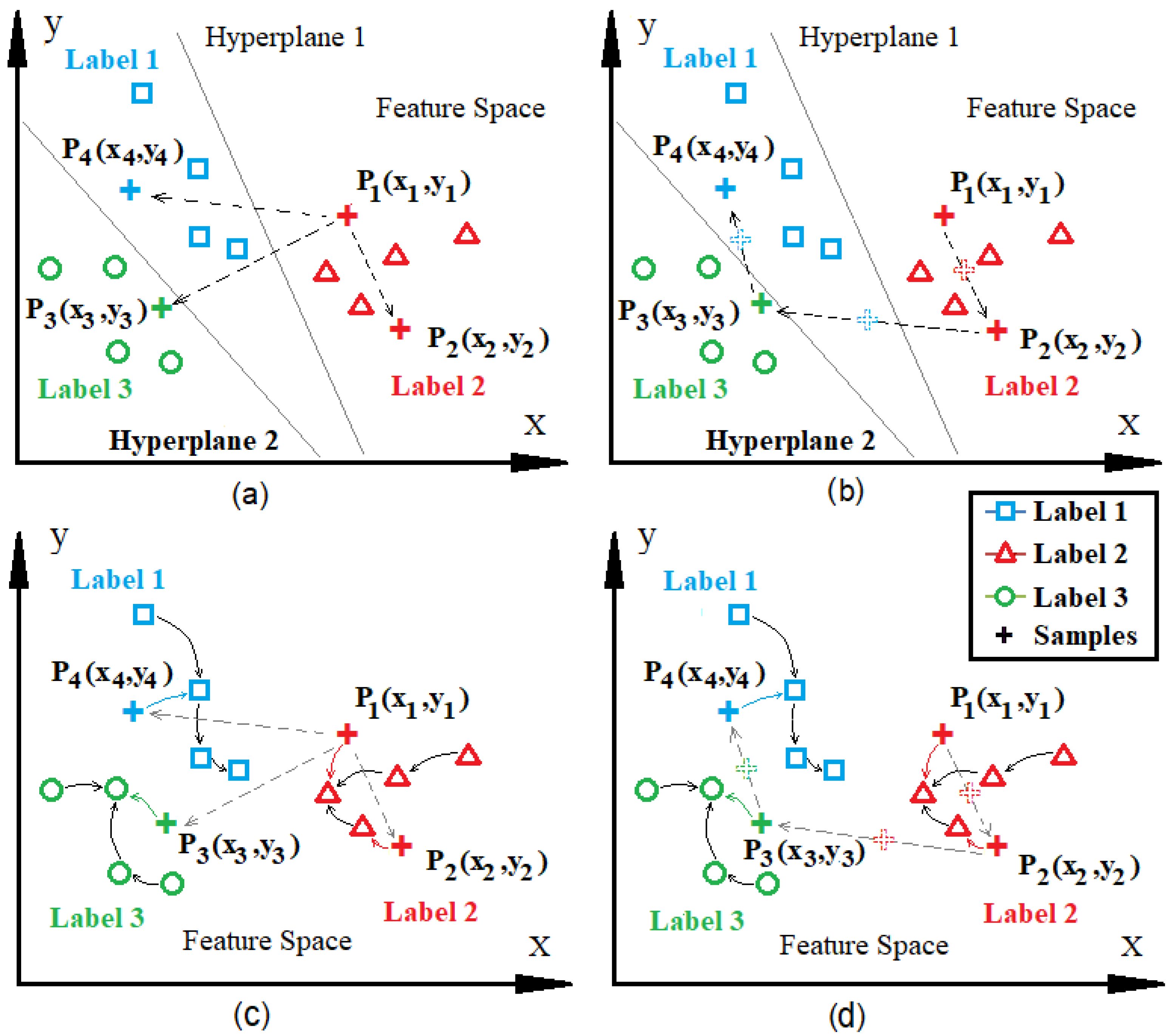
Once the feature space constructed by the classifier using labeled data is applied to recognize the patterns of new samples distributed within this structure, it is reasonable to assume that a new sample sharing the same features as one already included in the feature space will occupy the same position and receive the same label of that region, or will be classified according to its affinity with the nearest sample. If the feature values of the gases change, the same sample will relocate to a different position in the feature space and receive a label according to the heuristics or classification method of the algorithm. A simplified representation of a two-dimensional feature space with three labels is illustrated in Figure 1, where P1(x1,y1) represents the initial position of a new sample introduced into the space, and P ( x 2 , y 2 ) 2 , P ( x 3 , y 3 ) 3 , and P ( x 4 , y 4 ) 4 denote hypothetical positions that this sample may assume when its features—here represented by coordinates x and y—vary. If the values of x and y are discrete, transitions between positions will also occur discretely within the classifier (Figure 1a,c). Conversely, if the values are continuous, the position changes will be smooth, defining a trajectory that passes through all positions from P1 to P4 (Figure 1b,d).
In the case of fault classification using DGA, changes in the values of gas features in a sample determine its repositioning within the feature space between P1 and P4, as faults may evolve from less to more severe conditions, or in some cases, diminish entirely. Therefore, since increases in gas concentrations are a key indicator of incipient fault diagnosis [2,3], continuous monitoring with regular intervals (e.g., monthly or weekly) between DGA analyses of a transformer enables tracking the trajectory of successive readings over time within the feature space of classifier algorithms. Because it is possible to determine both the distance and chronological order of these samples relative to the hyperplanes separating different classes or labels (Figure 1b), or the strength of the connectivity relations between nearby samples (Figure 1d), it becomes feasible not only to assign labels to the samples but also to identify trends and behavioral variations of gases associated with faults. In this analytical context, both KNN (with K = 1 ) and OPF were applied to explore the feature space. These algorithms were chosen not only for their simplicity but also because they can address multiclass problems without requiring complex configurations. Moreover, the heuristics used to construct the different regions of the feature space—regardless of their shape—incorporate distance as a key parameter for analysis and classification.
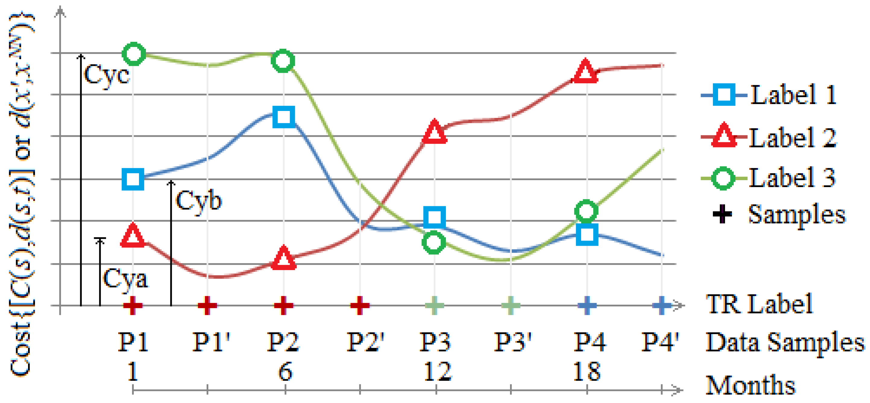
Thus, because the testing set consists of successive gas analyses performed at different periods or measurement dates as part of predictive maintenance routines, the graphical representation of the operational state of a given transformer TR, along with the gas evolution, can be hypothetically illustrated by a fault trend curve (Figure 2) corresponding to the DGA analysis dates. In this representation, the TR Label on the x-axis corresponds to successive measurements, i.e., DGA samples analyzed by the 1NN and OPF algorithms using monthly data points P1, P1, P2, …, P4. The y-axis represents the cost—expressed as [ C ( s ) , d ( s , t ) ] or d ( x , x N N ) —which is part of the classification heuristic and reflects the metric distance between samples along the TR Label axis and the various existing classes in the algorithms’ feature space. Accordingly, Cya, Cyb, and Cyc indicate the connectivity cost between the newly classified sample and the samples of different classes. A lower cost value indicates higher proximity and stronger connectivity to the corresponding class. Each TR sample submitted for classification is assigned the label of the existing sample in the feature space that yields the lowest cost. For instance, P1 is labeled as Class 2 because Cya < Cyb < Cyc. Since the costs are sequentially ordered (from lower to higher), they may be denoted as primary cost (main fault), secondary cost (second fault), and tertiary cost (third fault).
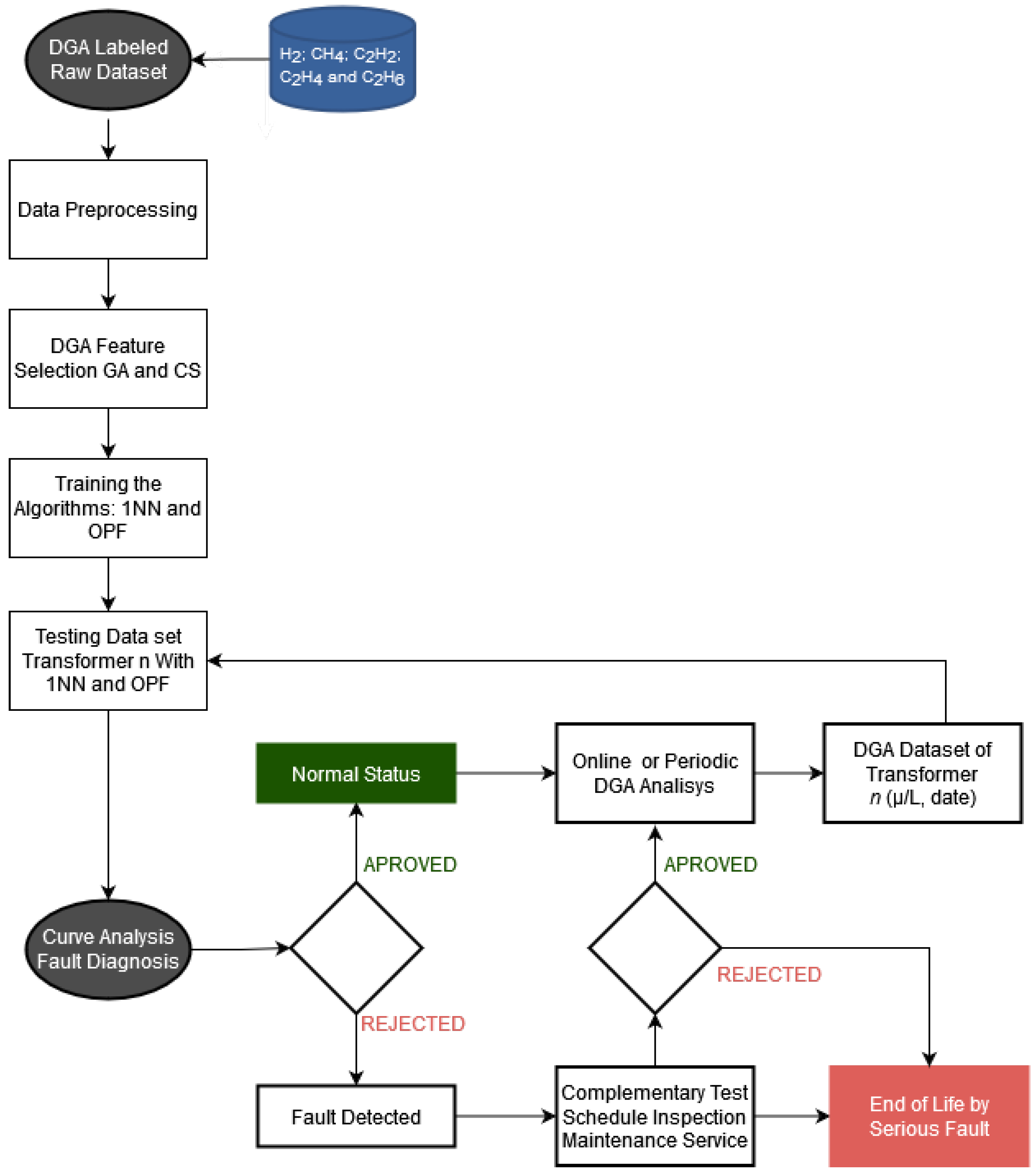
Analyzing fault behavior, it is observed that between P1 and P2, variations in the gas concentrations of TR samples caused repositioning within the feature space; however, the samples consistently retained the label of Class 2. It is noteworthy that between P2 and P2 there is a convergence of samples, indicating that the measurement at P2 is moving toward a transition zone (or confusion region). In this region, even slight changes in gas concentrations may result in a label change and, consequently, a different fault classification, as observed in P3 and beyond. From a predictive maintenance perspective, this situation provides crucial information, signaling a trend toward fault occurrence. It indicates the need for more frequent monitoring of TR from P2 onward, either by shortening the analysis intervals, performing specific complementary tests, or scheduling inspections. Figure 3 presents the block diagram of the fault analysis and diagnostic process of the methodology proposed in this study.

4. Methodology and Experiments

4.1. Data Preprocessing, Extraction of New Features and Simulations

Preprocessing includes data cleaning, transformation, normalization, and the selection of new features. The dataset used in this study for algorithm training was compiled from IEC TC10 [25], IEEE Dataport [26], CPFL–Companhia Paulista de Força e Luz [27], and published studies [28,29]. It comprised a total of 2298 samples, including 2049 normal samples, 63 thermal faults at T   <   700   ° C, 47 thermal faults at T   >   700   ° C, 70 partial discharges and low-intensity discharges (PDLI), and 69 high-intensity discharges (HID), across five types of combustible gases (H2, CH4, C2H2, C2H4, and C2H6). CO and CO2 gases were excluded from this analysis because some of the data sources did not report their concentrations. The transformer data and inspection reports analyzed were provided by a Brazilian electricity company.
Real-world data may be incomplete, inconsistent, and subject to errors or outliers; therefore, data cleaning is an essential step [30]. In this study, the impact of outliers on the performance of 1NN and OPF algorithms was minimized through dataset cleaning, specifically by removing samples that contributed to classification errors. The cleaning process was carried out using a normal probability distribution, with the 95th percentile calculated from the normal samples included in the dataset composition.
Table A2 presents the concentration values of the normal distribution in μ L/L, calculated for the 66th, 95th and 97.5th percentiles, based on the analysis of 2049 normal samples. According to IEEE Standard C57.104 [2], normal gas values are defined between the 90th and 95th percentiles. Thus, by applying the gas limit values from the 95th percentile (Table A1) to the transformer fault data, approximately 19 samples that could have been incorrectly classified as normal were eliminated. After data cleaning, the updated dataset consisted of 1818 normal samples, 44 thermal faults with T   <   700   ° C, 47 thermal faults with T   >   700   ° C, 70 PDLI cases, and 69 HID cases (see Appendix A for detailed results).
Table A3 presents the accuracy values of KNN and OPF obtained before (2298 samples) and after (2048 samples) dataset cleaning, under the following conditions: 5 gas types, 5 labels (classes), 100 simulations each, normalized data (mean and standard deviation), and 5-fold cross-validation. In [31], the accuracy of KNN and OPF was evaluated on several artificial and real datasets unrelated to DGA, where the 1NN configuration showed slightly better performance than OPF. This finding is consistent with the results in Table A3 for the gas dataset analyzed, where KNN with K = 1 achieved higher accuracy than OPF across different label types (see Appendix A for detailed results).
In the data transformation stage, following the approach proposed in [9], 10 additional features were derived from the 5 combustible gases by employing their total relative values and gas ratios commonly used in classical methods: H2, CH4, C2H2, C2H4, C2H6, C2H2/CH4, C2H2/C2H4, CH4/H2, C2H4/C2H6, C2H6/CH4, H2/Tg, CH4/Tg, C2H2/Tg, C2H4/Tg, and C2H6/Tg, where Tg = H2 + CH4 + C2H2 + C2H4 + C2H6. Feature selection for training and testing the proposed methodology was carried out by identifying the best subsets and combinations using the binary algorithms GA and CS, which resulted in improved accuracy. The accuracy of the 1NN algorithm was adopted as the fitness function in the optimization algorithms, since it demonstrated superior performance compared to OPF. Table A4 presents the parameter adjustments applied to the GA and CS algorithms, along with the results obtained for the preprocessed dataset. The minimum and maximum limits for feature combinations ranged from 6 to 10 gases; however, the most consistent and accurate results in both cases were achieved with 8 gas combinations (see Appendix A for detailed results).
Table A5 presents simulations using other machine learning algorithms, which apply different classification strategies to assess the risk of overfitting on the data obtained after feature selection. The evaluation was carried out under the condition of 5-fold cross-validation, and accuracy was calculated for unbalanced data using Equation (1). As observed, most of the algorithms achieved improved accuracy with 8 selected features, thereby ruling out the possibility of overfitting in the case of 1NN (see Appendix A for detailed results).
Table A6 presents the confusion matrices obtained from the average classification results using the raw dataset and feature selection with the 1NN algorithm, and feature selection alone with the OPF algorithm. In this analysis, accuracy was evaluated under different labeling schemes: 2 labels (normal state and fault), 3 labels (normal state, thermal fault, and electrical fault), and 5 labels as previously described. It was observed that in the preprocessed cases (95th percentile), accuracy improved compared to the raw data. The most significant impact was seen in the data for thermal faults < 700   ° C and normal states—where cleaning was performed—as well as in the upper range of low-intensity electrical faults. It was also observed that the two-class labeling approach achieved the highest accuracy, followed by the three-class and five-class approaches (see Appendix A for detailed results).
Therefore, using the validated training dataset with 8 selected DGA features, simulations were conducted on different sets of transformer gas samples collected over defined time intervals as part of the monitoring and predictive maintenance activities carried out by the electricity company.
The results were presented in three graphs: (i) gas concentration in μ L/L (PPM) and fault trends showing the behavior between normal and fault states; (ii) normal state, electrical fault, and thermal fault; and (iii) normal state along with five specific fault types.

4.2. Experiments Results

4.2.1. Case Study 1—345/88kV @133.33MVA

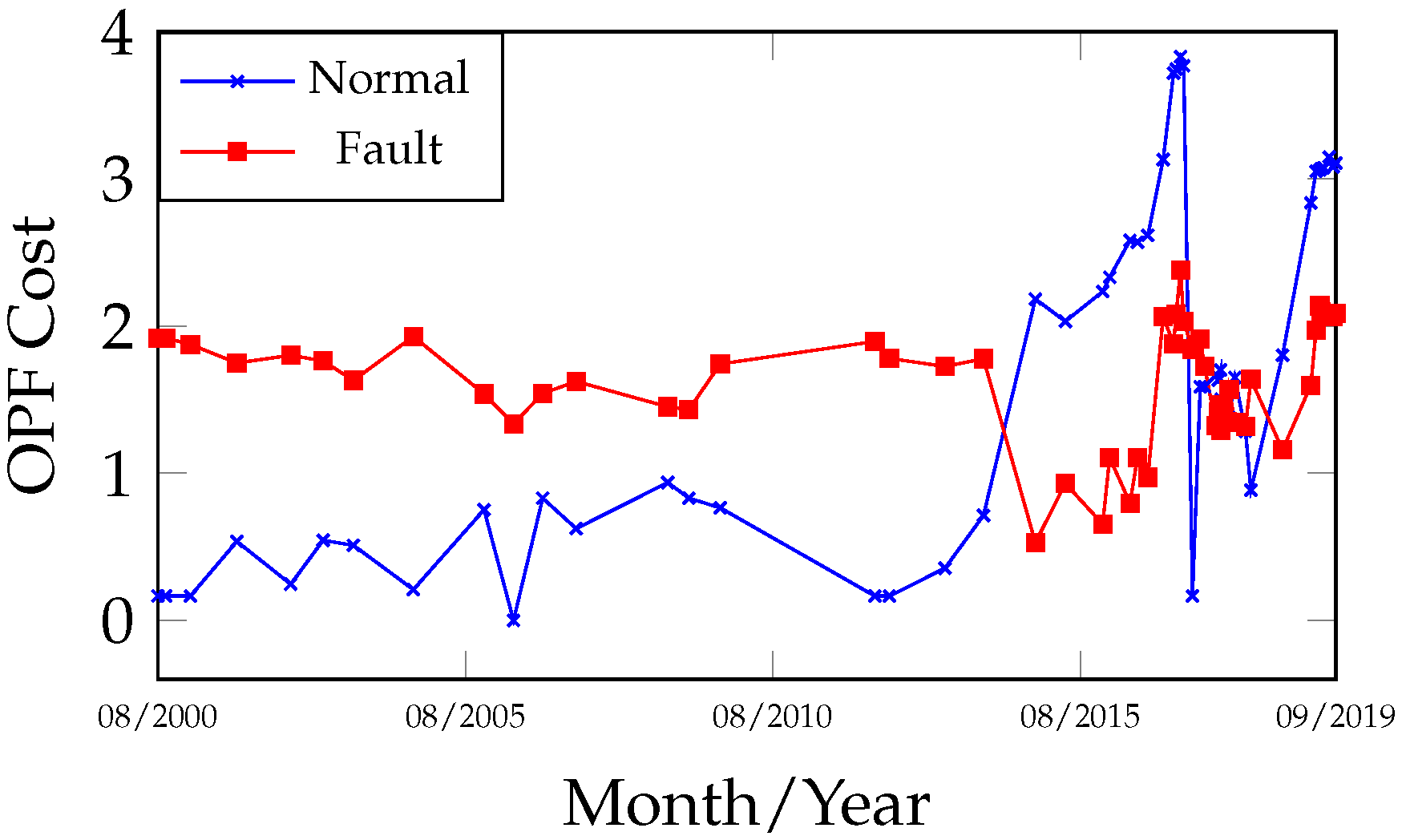
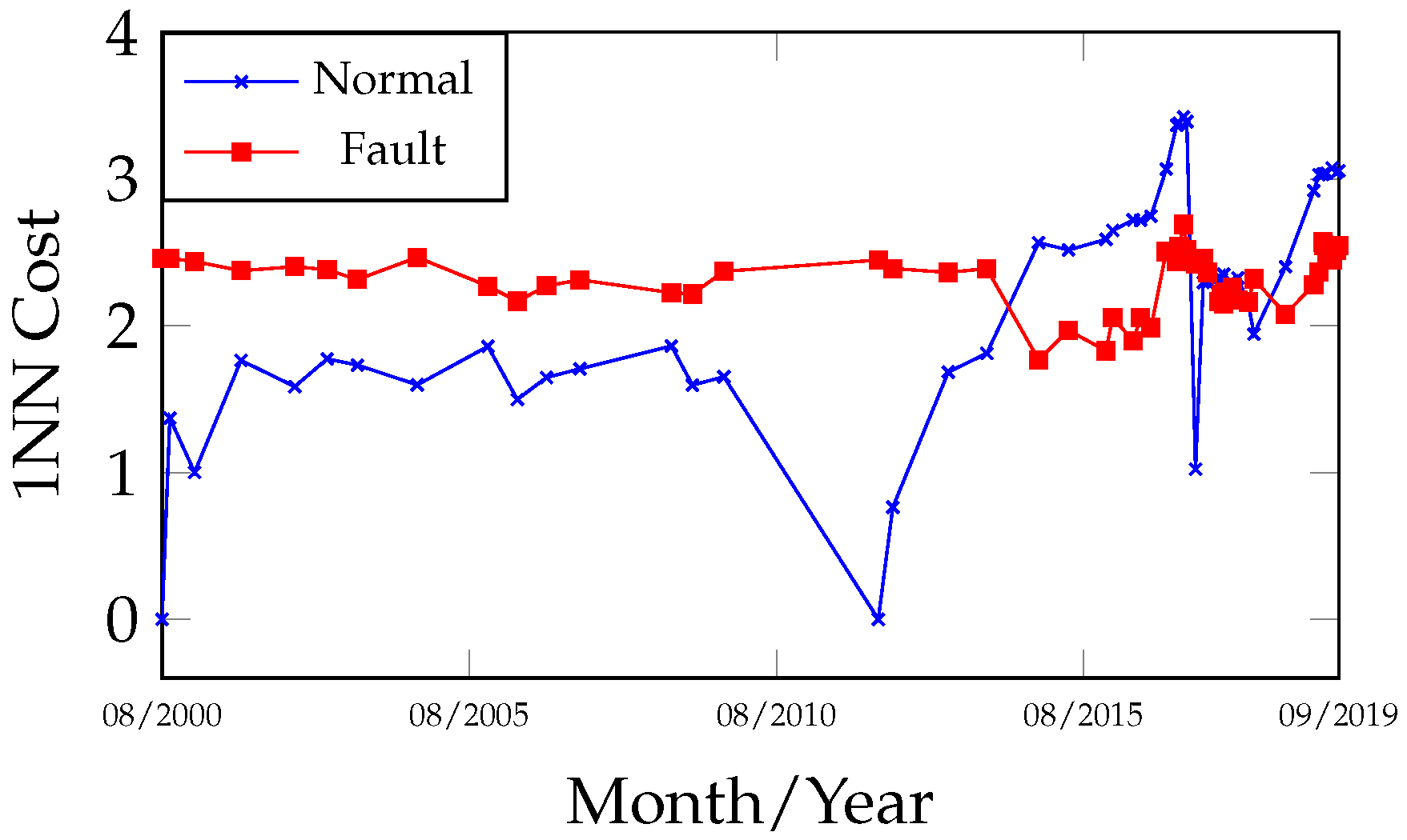
Figure 4 presents the DGA record for the equipment over the operational period from 4 August 2000 to 30 September 2019. On 1 April 2012, an oil treatment was carried out to improve its physicochemical properties and remove dissolved gases. After the equipment returned to operation, the gas evolution observed in the 15 December 2015 analysis prompted a reduction in the monitoring interval from semi-annual to quarterly, and subsequently to monthly after 8 December 2016, due to the high gas concentrations detected. An internal inspection of the equipment was performed by the electricity company only on 9 April 2017.
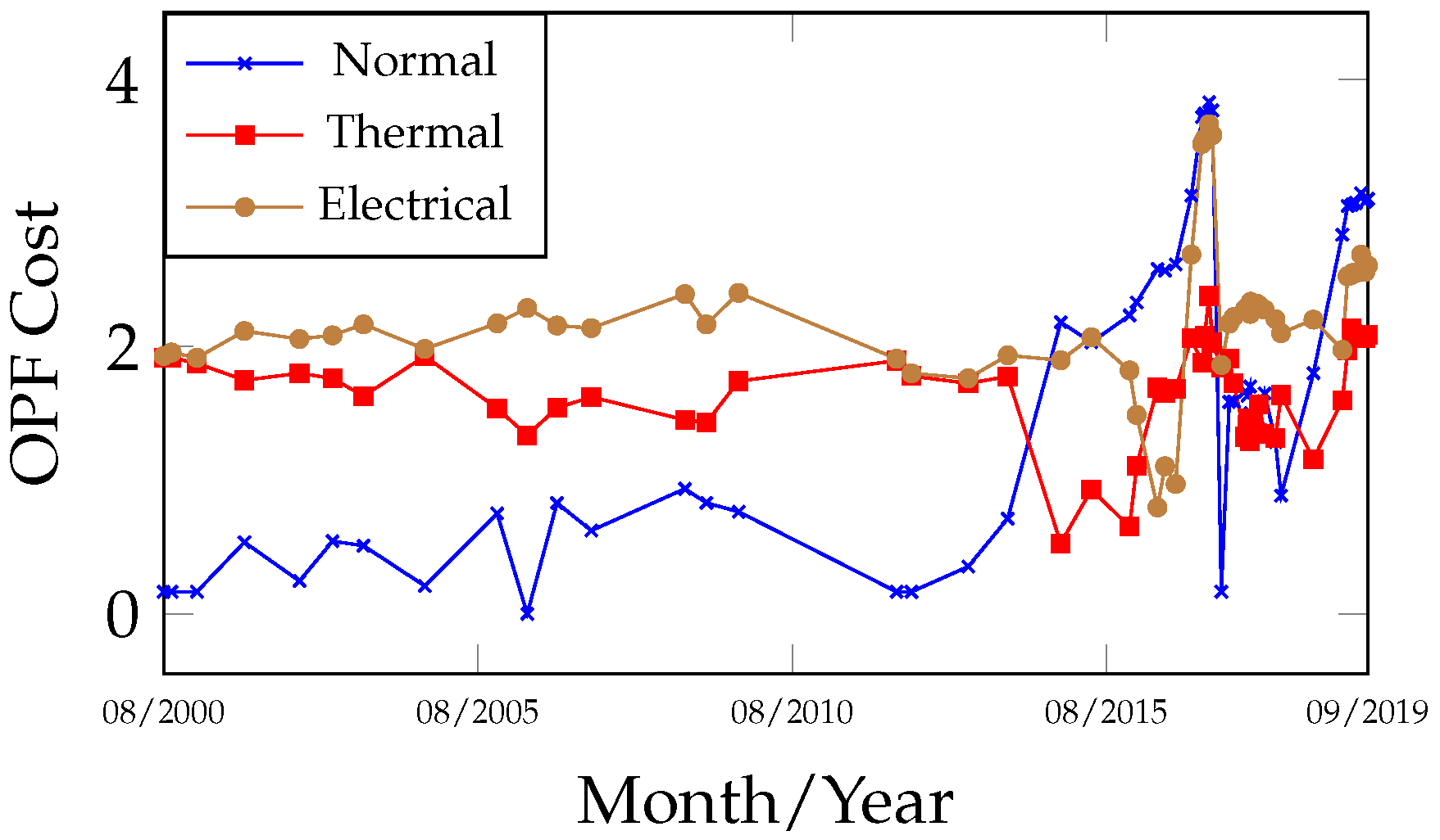
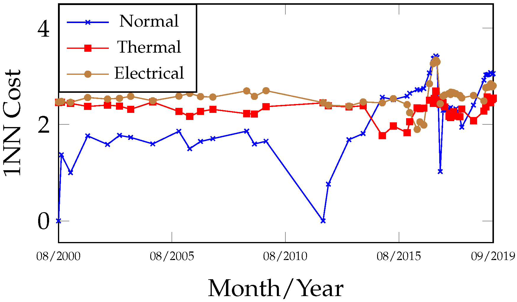
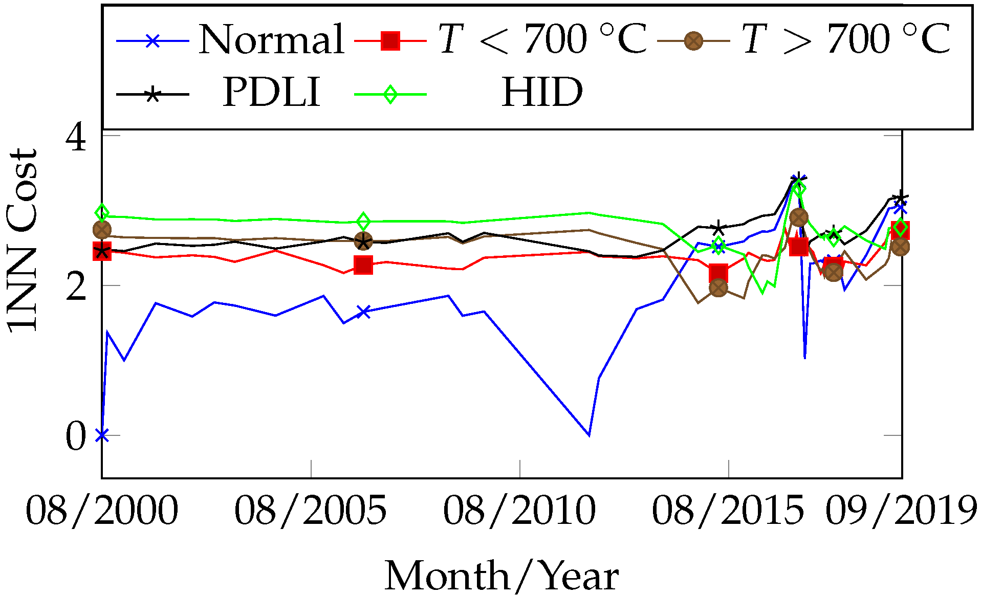
Analyzing the fault evolution curves (Figure 5 and Figure 6) for the dates 4 August 2000 and 1 April 2012, the stability and low gas concentrations in the samples evaluated by 1NN and OPF were classified as normal, as they exhibited lower cost values and were distant from the fault class within the observed interval between both curves. After the oil treatment, as gas concentrations increased, an approximation was observed between the normal curve (increasing cost) and the fault curve (decreasing cost), indicating a transition from a normal to a fault state, which occurred between 6 January 2014 and 10 November 2014, prior to the transformer’s internal inspection. Complementing Figure 5 and Figure 6, the curves in Figure 7 and Figure 8 enable the identification of the fault group involved, distinguishing between thermal and electrical faults. In this case, indications of both fault groups were observed during the period. The primary gases produced during the fault signals were CH4 and C2H4 (Figure 4), which are typically associated with thermal faults when predominant, and of moderate relevance in electrical faults. Figure 9 and Figure 10 complement the previously discussed fault curves by specifying the fault classes, revealing signals of thermal faults ( T < 700   ° C and T > 700   ° C) and high-intensity electrical discharges occurring throughout most of the transformer’s operational period. The curves from Figure 5, Figure 6, Figure 7, Figure 8, Figure 9 and Figure 10 are complementary, although they may also be interpreted independently. A comparison of the fault curves obtained from the 1NN and OPF algorithms reveals a high degree of similarity in both behavior and results.
During the internal inspection (opening) of the equipment on 9 April 2017, carbon particles were found on the shaft drive surface of the no-load tap changer, and the copper braided wire of the busbar TAP exhibited discoloration and partial breakage of its strands, providing clear evidence of overheating at T > 700   ° C. Relating the fault evidence identified in the transformer to the proposed methodology, the heating issue likely began after 6 January 2014, as indicated by Figure 5, Figure 6, Figure 7, Figure 8, Figure 9 and Figure 10. The signal of a high-intensity electrical fault (HID) may be interpreted as a classification error within the accuracy margin of the algorithms (Table A6).
The classification obtained on 8 December 2016, which preceded the inspection, shifted to T < 700 °C due to changes in gas concentrations, representing a new classification error. However, from a curve analysis perspective, it is important to note that after 8 December 2016 in the fault hierarchy of Figure 9 and Figure 10, the secondary fault T > 700 °C appears close to the primary T < 700 °C. Similarly, during the period from 6 January 2014 to 10 November 2014 in Figure 5, Figure 6, Figure 7, Figure 8, Figure 9 and Figure 10, the faults closest to the primary electrical fault were thermal (secondary and tertiary faults). In summary, the curves allow the establishment of a sequence of possible faults. After the transformer resumed operation, all fault trend curves (Figure 5, Figure 6, Figure 7, Figure 8, Figure 9 and Figure 10) after 31 May 2017 exhibited a period of curve proximity alternating between normal and fault states. This behavior is associated with the homogenization period of residual gases within the oil-impregnated paper. Nevertheless, on 17 November 2018, a new gas evolution was detected, along with an indication of a thermal fault trend: T > 700 °C (primary) and T < 700 °C (secondary). This finding suggests the need for closer monitoring with more frequent analyses until a new internal inspection is performed.

4.2.2. Case Study 2—Tranformer 230/88kV @50MVA

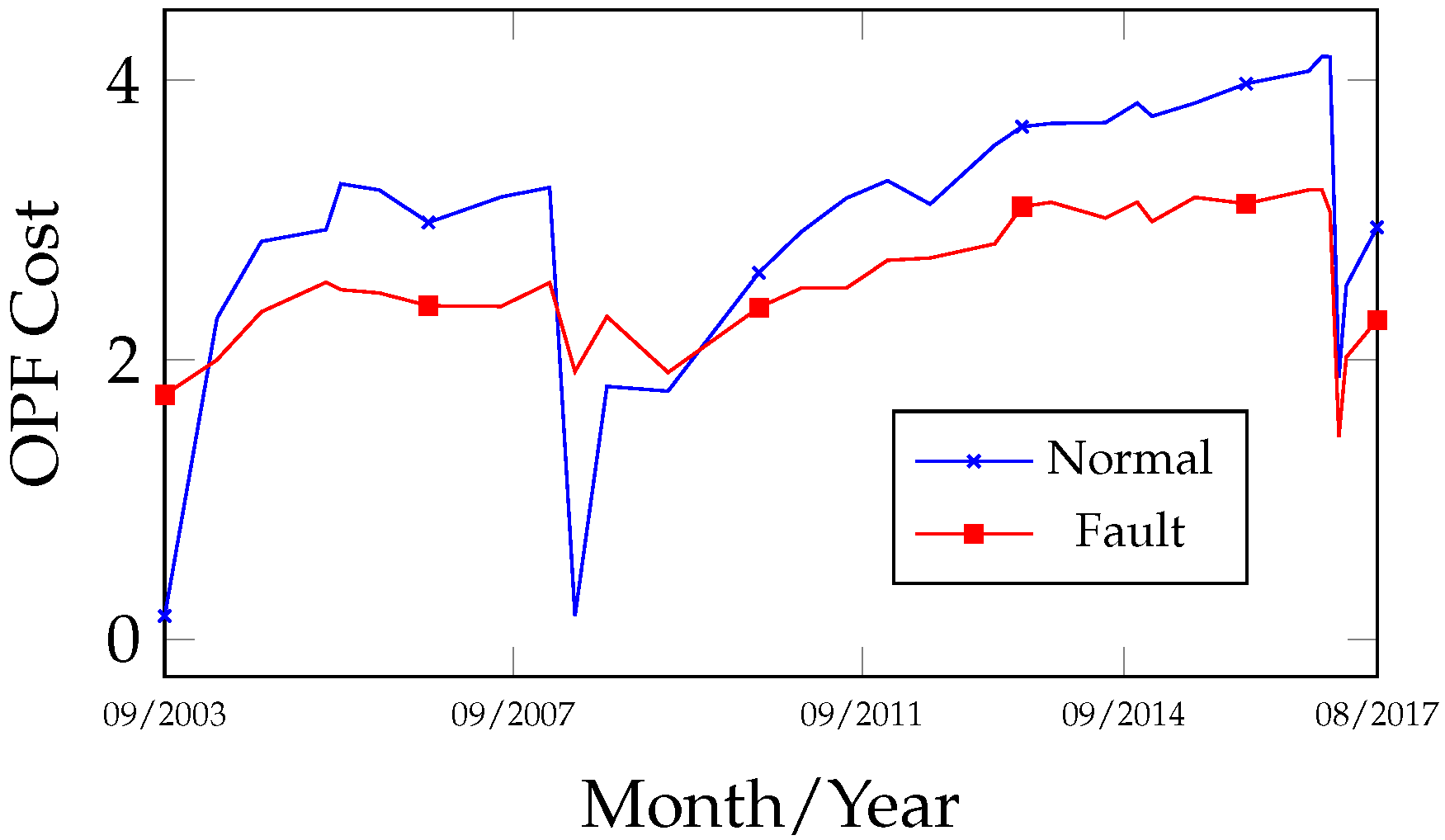
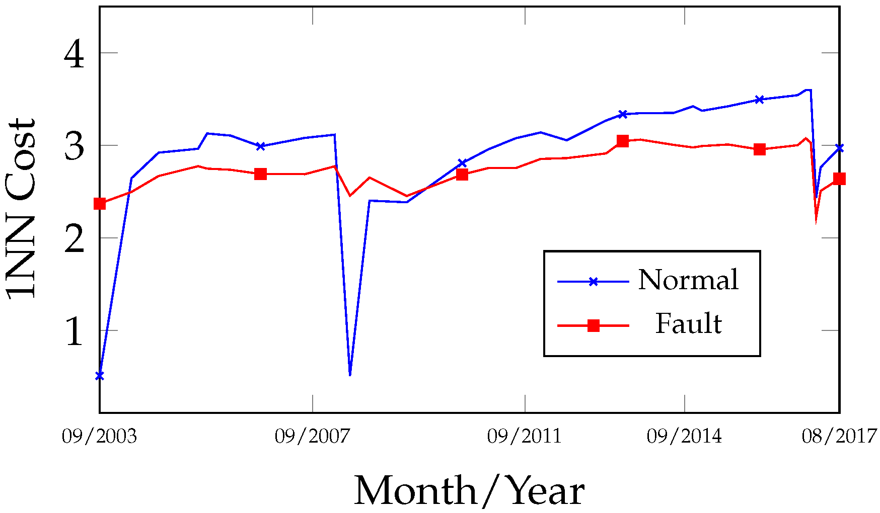
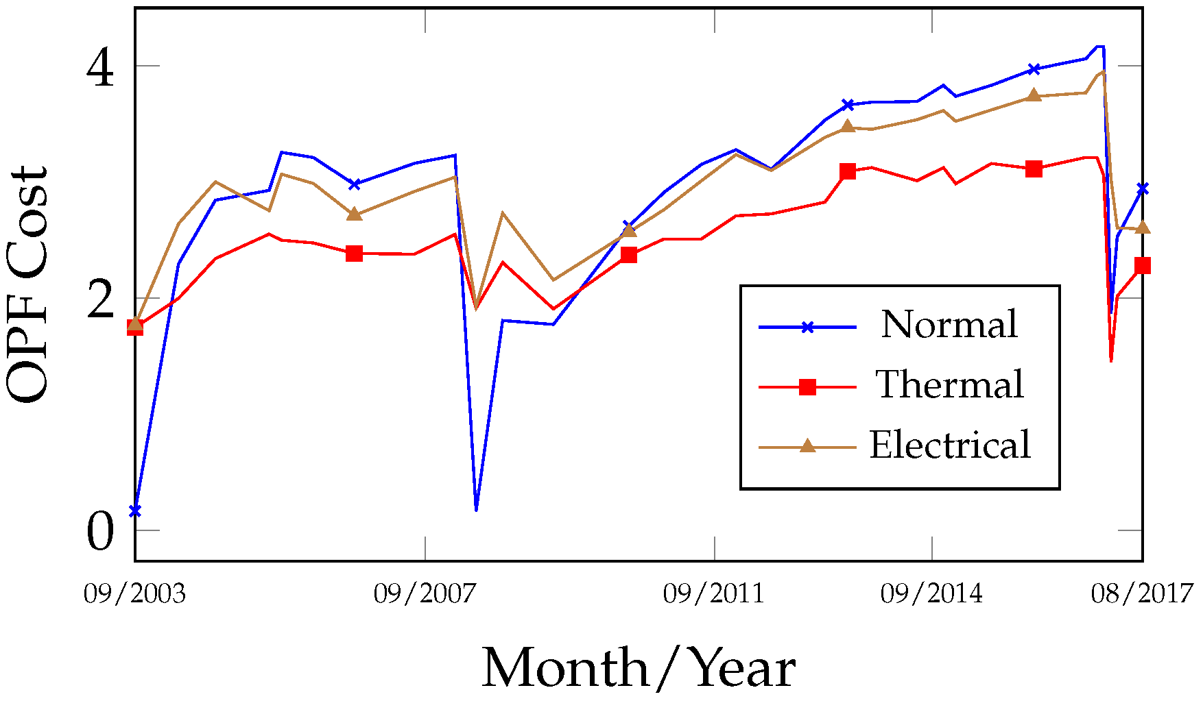
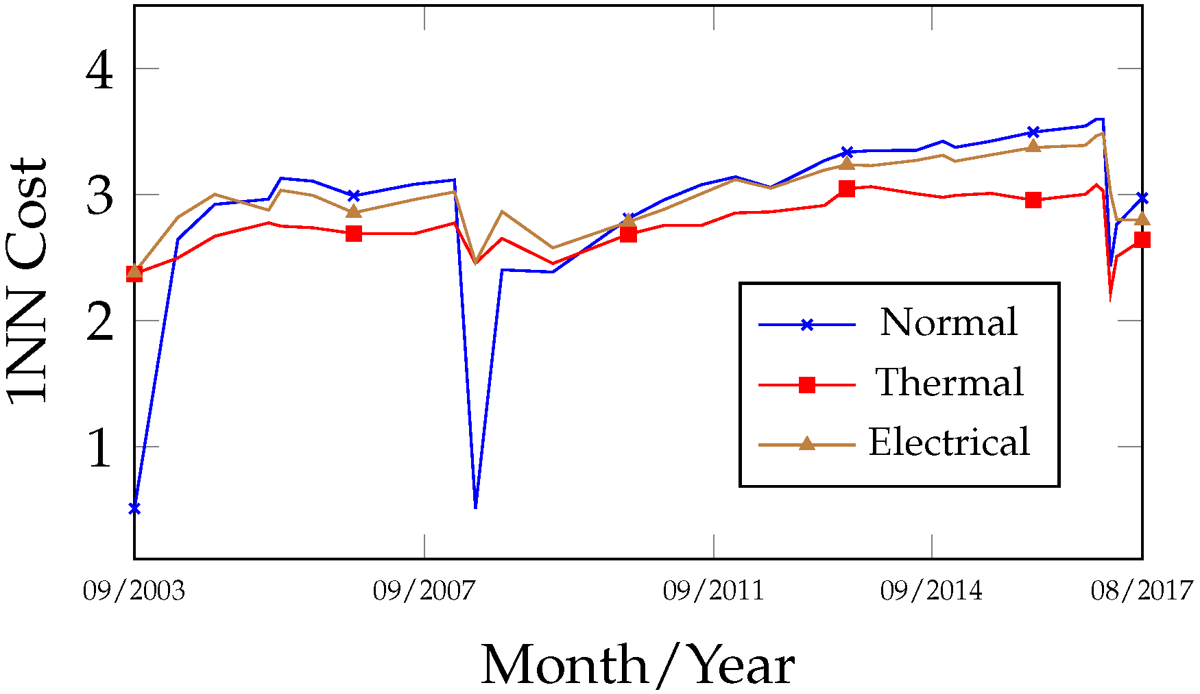
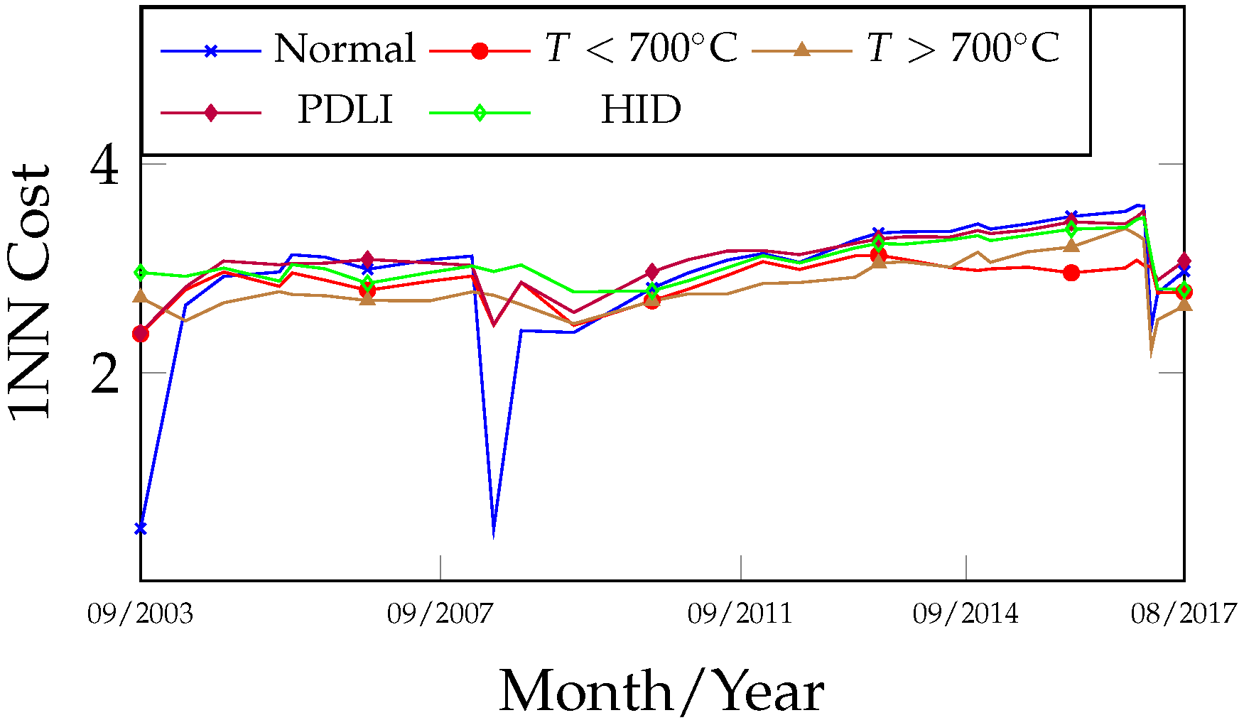
Figure 11 presents the record of gas analyses during the equipment’s operational period from 28 September 2003 to 25 August 2017. On 12 June 2008, the insulating oil was treated to improve its physicochemical properties and remove dissolved gases. Despite the gas evolution observed after the equipment returned to operation, the DGA analysis interval was maintained on a biannual basis until 23 February 2016, after which it was changed to a monthly interval until 9 February 2017, when an internal inspection was performed and maintenance was carried out by the electricity company.
Analyzing the fault trend curves in Figure 12 and Figure 13, it can be observed that as soon as the equipment began operation, on 4 May 2004, the curve already indicated the presence of a fault, and on 27 February 2008 the operation was interrupted for an oil treatment.
It is noteworthy that during this period no inspection activities were performed, probably due to the stabilization of gas evolution preceding the treatment, a condition often associated with the natural disappearance of the fault.
After 7 July 2009, a new increase in gas concentration was observed, with fault indications occurring between 23 July 2010 and the equipment opening after 9 February 2017.
The fault evolution curves in Figure 14 and Figure 15 indicate that all faults occurring between 28 September 2003 and 25 August 2017 were classified as thermal (lower cost).
The relevant gases detected during this period were H2, CH4, and C2H4, along with moderate amounts of C2H6 and traces of C2H2. Depending on their concentration, these gases may be associated with thermal faults or low/high energy discharges.
In the recognition of specific fault classes, the analyses of the curves in Figure 16 and Figure 17 reveal that alternate thermal faults occurred at different times: between 4 May 2004 and 27 February 2008, and from 23 July 2010 to 17 July 2014, thermal faults with T > 700 °C were detected, while from 17 July 2014 to 9 February 2017, thermal faults with T < 700 °C were identified.
A high degree of similarity was also verified in the behavior and results obtained between the 1NN and OPF algorithms.
During the internal inspection conducted after 9 February 2017, several occurrences with thermal fault characteristics were identified, indicating both medium- and long-term manifestations. These findings revealed degradation of the paper insulation (carbonized and lost dielectric properties) caused by overheating ( T < 700   ° C) on the X1 and X2 low-voltage bushings, with recent fault characteristics. Additionally, signs of heating were observed in the form of discoloration on screws and partial fusion of a washer on the core clamping frame ( T > 700   ° C), the latter probably originating prior to 27 February 2008, as suggested by the degree of degradation. In this context, the results obtained demonstrate consistency; however, it is noteworthy that both thermal faults (primary and secondary) consistently occurred in close proximity throughout the entire period analyzed. In November/2015, an acoustic emission test was carried out to investigate the presence of partial internal discharges associated with gas accumulation (mainly C2H2). Although no anomalies were detected, the test supported the conclusion that the fault identified prior to November/2015 was most likely thermal in nature.

4.2.3. Case Study 3—440/138kV @100MVA

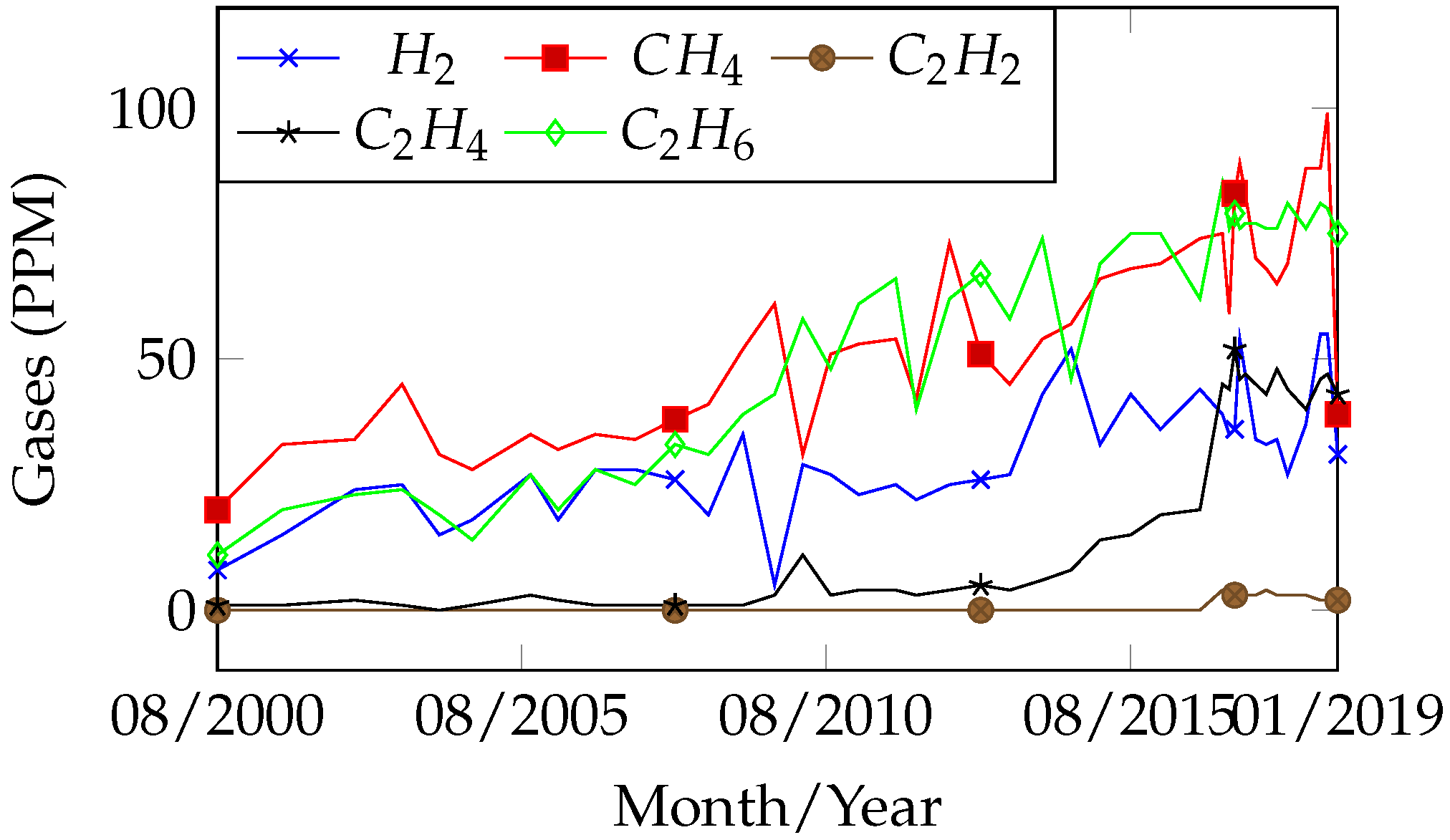
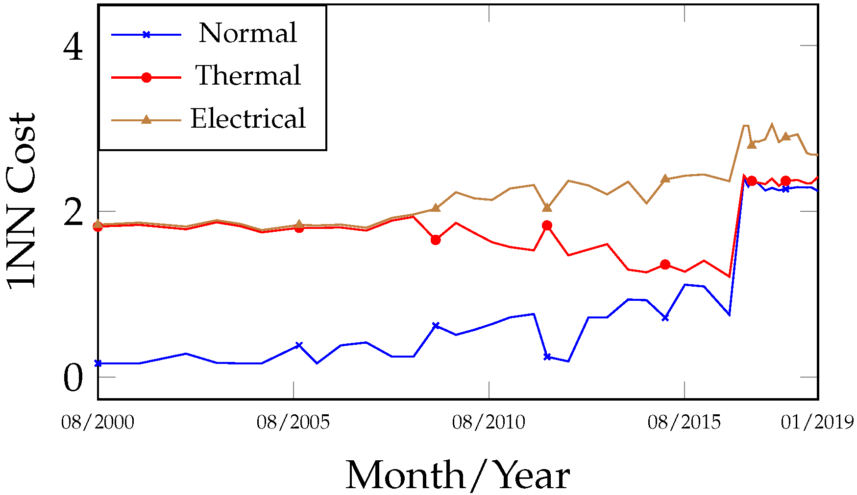
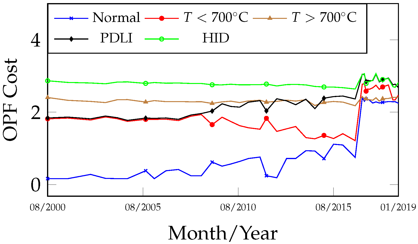
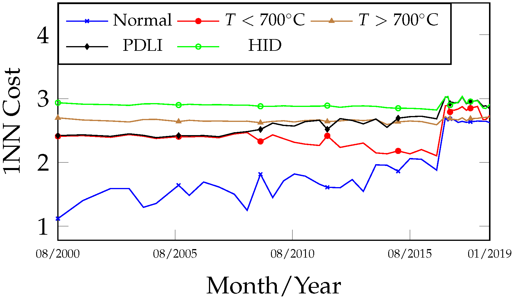
Figure 18 presents the record of gas concentration analysis throughout the operational life of the equipment, spanning from 7 August 2000 to 2 January 2019. This case refers to a transformer operating under normal conditions in the electrical system, with no anomalies recorded. In its DGA analysis, a slow increase in gas concentration can be observed; however, from 9 February 2017, there was a slight rise in CH4 and C2H6 concentrations, along with the emergence of C2H2, which is typically associated with electrical faults when significant, or with thermal faults at T < 700   ° C in smaller amounts. The presence of C2H2 is regarded as an aggravating factor for faults, generally requiring closer monitoring of the equipment. Consequently, the interval between DGA analyses is reduced to monthly. After 26 June 2017, with the stabilization of gas evolution, the analysis frequency was changed back to quarterly.
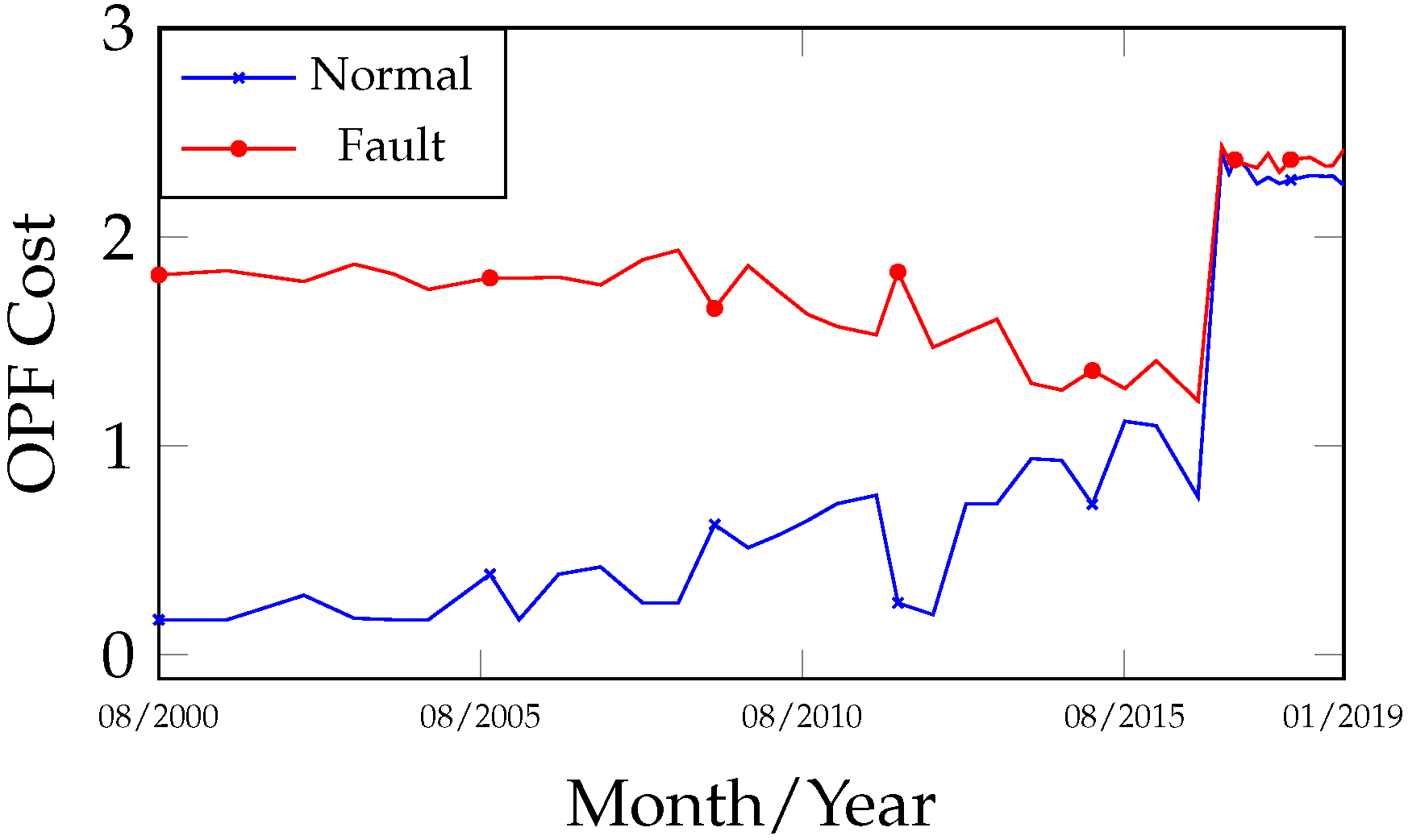
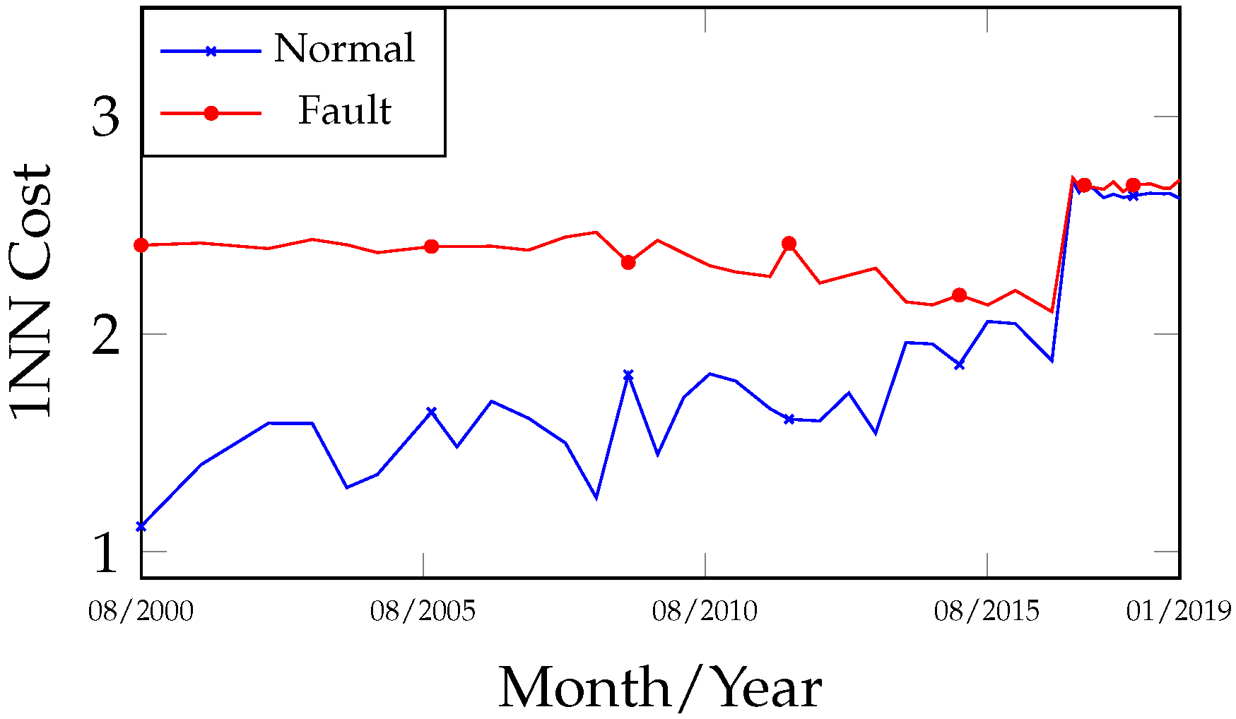
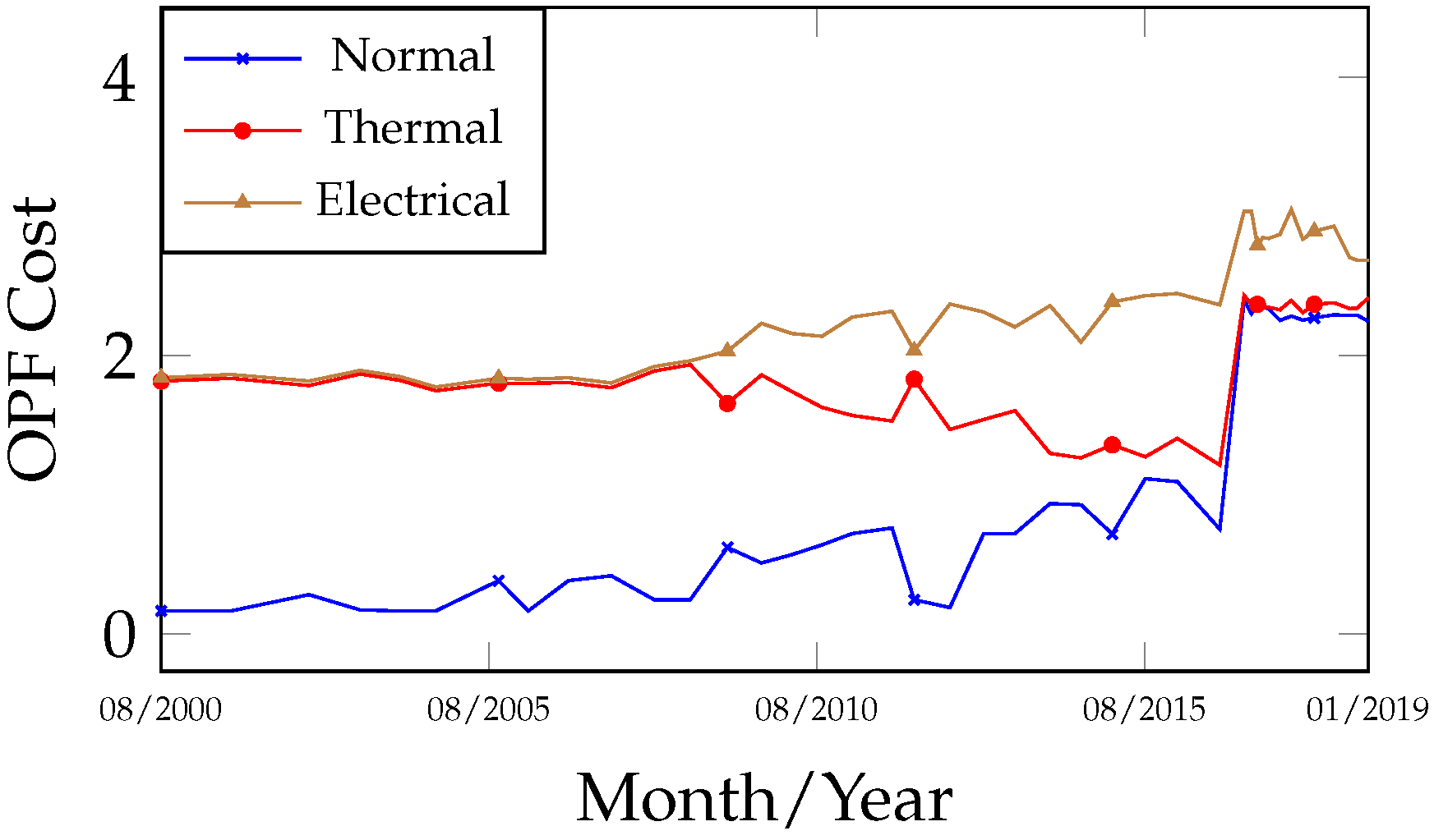
In the fault evolution curves of Figure 19 and Figure 20, between 7 August 2000 and 27 September 2016, it is possible to observe the convergence of the fault and normal curves as the gases evolved. On 9 February 2017, with the emergence of C2H2 gas in association with H2, CH4, and C2H6, a sudden convergence of the curves occurred, indicating that any variation in gas concentration could shift the state from normal to fault. Therefore, it was justifiable to adopt more rigorous monitoring. In the curves of Figure 21 and Figure 22, the evaluated samples are classified as normal between 7 August 2000 and 27 September 2016; however, they display a trend toward approximation with the thermal fault and distancing from the electrical fault. This behavior can be explained by the presence of CH4 and C2H6, which are typical of a thermal fault at T < 300   ° C. It is important to note, however, that the growth of these gases may also be associated with normal operating conditions, such as equipment overload leading to stray gassing. Nevertheless, in the analyzed transformer, the presence of C2H2 is not typical of normal operation and should be treated with caution when detected, since it contributes to the indication of a secondary fault, which shifted to T > 700   ° C after 9 February 2017, as illustrated in the curves of Figure 23 and Figure 24. After the 1 November 2008 analysis, a decrease in gas concentration was observed, initiating a gradual separation between the normal and fault states. When comparing the results of the fault curves obtained by 1NN and OPF, the behaviors and outcomes were once again very similar.

4.2.4. Others Experiments Results

Other pieces of equipment were analyzed using the method proposed in this paper, and Table A7 presents a summary of the predicted and actual faults identified during internal inspections (equipment opening) performed on the transformers. Analyzing the results, it can be observed that for all evaluated equipment, the diagnostic accuracy regarding fault presence—based on the analysis of the Normal vs. Fault curves—was 100.00%. For the Normal vs. Fault Thermal and Electrical condition, the accuracy reached 88.90%, while for the Normal vs. 5 Faults condition, it was 66.70%. These outcomes can be considered satisfactory, highlighting the distinguishing advantage of fault trend analysis, which reveals both primary and secondary faults. It is important to emphasize that a well-labeled dataset is a necessary prerequisite and exerts a strong influence on the final results (see Appendix A for the table of results).
5. Conclusions

Unlike conventional DGA interpretation methods using machine learning algorithms, which merely assign a label (class) to specific fault types occurring in transformers based on successive analyses of gas evolution samples, the proposed dissolved gas interpretation method explores the feature space and classification heuristics of OPF and KNN algorithms, converting them into graphical representations that enable behavioral analysis of different types of incipient faults throughout the operational life of the transformer.
This characteristic makes it possible to estimate the trend of potential fault situations, not limited to a single class type, but by observing the sequence of faults determined by their associated costs, ranging from lower (main fault) to higher (secondary, tertiary, and other faults). In this way, the method provides insight into the possible proximity scenarios among them.
In these cases, the use of three different curves for recognizing the evolution of fault types aims to simplify the analysis and more effectively explore the gas information, as they are subjected to varying levels of accuracy. Specifically, for all evaluated transformers, the diagnostic accuracy was 100.00% for two classes (normal and fault), 91.20% for three classes, and 66.67% for five classes.
When compared with results reported by other authors, the proposed method demonstrates competitive and, in some cases, superior performance. For instance, Ref. [8] reported 76% accuracy with Multilayer ANN and 81.4% with SVM applied to DGA data. More recently, Ref. [11] introduced a causal reasoning framework reaching 95.8%. In this context, our method achieved 100% accuracy in binary classification (normal/fault), surpassing traditional machine learning models, and provided robust performance for three-class classification (91.20%), which is comparable to the most advanced approaches in the literature. Although the five-class scenario reached 66.67%, the method still offers valuable insights by enabling graphical behavioral analysis throughout the transformer’s operational life, something not addressed by conventional classification techniques.
Thus, with knowledge of this information, it becomes possible to plan new maintenance actions, including specific complementary tests, and to schedule inspections and maintenance in order to reduce the likelihood of unexpected transformer removal from the electrical system due to a fault.
Although the proposed methodology was validated using historical datasets, it is worth highlighting that the framework can be extended to real-time applications. The integration of online monitoring data would enable continuous assessment of transformer conditions, allowing not only fault detection but also the prediction of state evolution and the identification of incipient trends. This perspective opens opportunities for further development of the method as an advanced tool for predictive maintenance in power transformers.
Regarding the 1NN and OPF algorithms, both exhibited strong similarities in their results, which supports the use of either algorithm for the diagnosis of incipient faults in transformers.
Although the proposed methodology was validated using historical datasets, it is worth highlighting that the framework can be extended to real-time applications. Future work will analyze the behavior of the classifiers by employing hyperplanes in the construction of the feature space. Moreover, the integration of online monitoring data would enable continuous assessment of transformer conditions, allowing not only fault detection but also the prediction of state evolution and the identification of incipient trends. This perspective opens opportunities for further development of the method as an advanced tool for predictive maintenance in power transformers.

Author Contributions

Conceptualization, A.G. and M.A.I.; methodology, A.G. and M.A.I.; software, A.N.d.S.; validation, A.G., M.A.I. and F.T.N.; formal analysis, A.N.d.S.; investigation, D.S.G.; resources, V.H.S.Y. and W.B.; data curation, M.A.I.; writing—original draft preparation, A.N.d.S.; writing—review and editing, F.T.N. and P.d.C.J.; visualization, D.S.G. and A.N.d.S.; supervision, T.M.; project administration, P.d.C.J.; funding acquisition, T.M. All authors have read and agreed to the published version of the manuscript.

Funding

This work was supported by São Paulo State University (UNESP), Brazil.

Institutional Review Board Statement

Not applicable.

Informed Consent Statement

Not applicable.

Data Availability Statement

No data is used in this article.

Acknowledgments

The authors would like to thank the financial support via São Paulo State University—UNESP—PROPe.

Conflicts of Interest

The authors declare that they have no competing interest.

Abbreviations

The following abbreviations are used in this manuscript:
1NN1-Nearest Neighbor
1D-CNNOne-Dimensional Convolutional Neural Network
ANNArtificial Neural Network
BPNNBackpropagation Neural Network
CORALCorrelation Alignment
CSCuckoo Search
DGADissolved Gas Analysis
DLDeep Learning
ELMExtreme Learning Machine
GAGenetic Algorithm
GSAGravitational Search Algorithm
GWOGray Wolf Optimization
HIDHigh Intensity Discharge
KNNk-Nearest Neighbors
LGBMLight Gradient Boosting Machine
LSTMLong Short-Term Memory
MLPMultilayer Perceptron
MMDMaximum Mean Discrepancy
MSTMinimum Spanning Tree
NNormal
NGO-GBDTNorthern Goshawk Optimization—Gradient Boosting Decision Tree
OPFOptimum-Path Forest
PCAPrincipal Component Analysis
PDLIPartial Discharges and Low-Intensity Discharges
PRNPattern Recognition Neural Network
PSOParticle Swarm Optimization
RBFRadial Basis Function
RFRandom Forest
SHAPSHapley Additive exPlanations
SVMSupport Vector Machine
TThermal Fault
T < 700 °CThermal Fault Below 700 °C
T > 700 °CThermal Fault Above 700 °C
TgTotal Combustible Gases
TEThermal and Electrical Fault
TRTransformer
XGBoostExtreme Gradient Boosting

Appendix A

Table A1. Gas importance by faults in power transformers (adapted from [2]).
Cause of Gas GenerationMain Gas TypeMedium Gas TypeMinor Gas Type
Catalytic reactions (<100 °C)H2--
Partial Discharge—CoronaH2-CH4, C2H6
Stray Gassing—T < 200 °CH2CH4C2H4, C2H6
Thermal fault—T < 300 °CC2H6CH4H2, C2H4
Overheating of paper 1 or mineral oilC2H6CH4H2, C2H4
Carbonization of paper 1CH4C2H4, C2H6H2
Thermal fault—300 °C < T < 700 °CCH4, C2H4H2, C2H6-
Thermal fault—T > 700 °CC2H4H2, CH4C2H2, C2H6
Discharge Low Energy or sparkingH2C2H2, C2H4CH4
Discharge High Energy (arcing)H2, C2H2CH4, C2H4-
1 Paper overheating, carbonization or aging can produce CO and CO2.
Table A2. Percentile of gas concentrations for normal samples classes ( μ L/L or PPM).
PercentileH2CH4C2H2C2H4C2H6
66th40.4347.380.6540.8976.04
95th66.8379.441.2067.15134.63
97.5th93.22111.501.7593.41193.22
Table A3. KNN and OPF accuracy for pre-processing and raw data.
AlgorithmDataset1NN3NN5NN7NN9NN
KNNRaw Data81.1 ± 2.8 @1NN77.8 ± 2.7 @3NN77.7 ± 2.9 @5NN77.5 ± 2.7 @7NN76.6 ± 2.7 @9NN
95th84.7 ± 2.8 @1NN82.0 ± 2.8 @3NN80.8 ± 2.8 @5NN80.7 ± 2.8 @7NN80.1 ± 2.9 @9NN
OPFRaw Data80.5 ± 3.1
95th84.0 ± 2.7
Table A4. Feature selection algorithm for 95th dataset with 5 fault types.
AlgorithmMinMaxBestBest Consistency (%)Mean Accuracy (%)Gas Ratio
CS + 1NN7985587.3 ± 2.7H2, CH4, C2H2, C2H4, C2H6, Tg, C2H2/CH4, C2H2/C2H4
GA + 1NN61083387.3 ± 2.8
Algorithms Parameters Configuration: 1NN@50 simulations, CS/GA@30 simulations and 20 iterations; CS: nests = 30, mutation number = 10, Levy coefficient λ = 1, step size α = 1; GA: particles = 30, mutation rate = 0.1, crossover rate = 0.9.
Table A5. Accuracy and Configuration of Classifiers with Selected Features.
AlgorithmFeaturesMean Accuracy (%)Basic Parameters Configurations for Best Accuracy (50 Simulations Each)
ANN MLP586.5 ± 1.41 hidden layer, 9 neurons, Levenberg–Marquardt, hyperbolic tangent
885.2 ± 1.51 hidden layer, 7 neurons, Levenberg–Marquardt, hyperbolic tangent
ELM kernel581.5 ± 0.8Regularization coefficient = 256, RBF kernel, kernel coefficient = 0.015625
883.0 ± 0.7Regularization coefficient = 4, RBF kernel, kernel coefficient = 0.015625
SVM kernel587.5 ± 0.8Regularization coefficient = 428.06, RBF kernel, kernel coefficient = 0.125220, one-vs-one strategy
888.6 ± 0.8Regularization coefficient = 0.191710, RBF kernel, kernel coefficient = 0.007785, one-vs-one strategy
Näive Bayes579.6 ± 0.8Kernel density estimation
882.0 ± 0.6
Table A6. Confusion matrix for 2, 3 and 5 status/fault diagnosis for 95th dataset.
AlgorithmDatasetFeatureLabelMean Accuracy (%)Status/Fault Confusion Matrix
NTE---
1NNRaw Data5291.4 ± 2.6N403.66.2---
TE7.842.0---
1NN95th8297.8 ± 1.5N363.20.4---
TE1.944.1---
OPF95th8297.7 ± 1.5N363.10.5---
TE1.944.1---
AlgorithmDatasetFeatureLabelMean Accuracy (%)Status/FaultNTE--
1NNRaw Data5388.2 ± 2.4N403.65.50.7--
T6.313.72.0--
E1.42.324.1--
1NN95th8394.1 ± 2.0N363.10.30.2--
T1.614.52.1--
E0.32.525.0--
OPF95th8394.1 ± 1.8N363.40.40.4--
T1.415.03.2--
E0.51.925.6--
AlgorithmDatasetFeatureLabelMean Accuracy (%)Status/FaultNT < 700 °CT > 700 °CPDLIHID
1NNRaw Data5381.1 ± 2.8N403.84.41.00.60.1
T < 700 °C5.34.51.31.30.3
T > 700 °C1.11.46.50.20.2
PDLI1.21.60.27.43.6
HID0.30.20.32.810.3
1NN95th5387.3 ± 2.7N363.20.00.30.10.1
T < 700 °C0.75.21.41.20.3
T > 700 °C0.80.97.00.40.2
PDLI0.01.40.39.62.7
HID0.20.30.52.310.5
OPF95th5386.9 ± 2.6N363.60.10.20.10.0
T < 700 °C0.54.52.11.40.4
T > 700 °C1.01.07.70.20.1
PDLI0.01.30.110.02.6
HID0.10.30.52.510.6
N—Normal, T—Thermal, E—Electrical, TE—Thermal + Electrical, PDLI—Partial Discharge and Low Intensity Discharge, HID—High Intensity Discharge, Thermal = T < 700 °C + T > 700 °C, Electrical = PDLI + HID.
Table A7. Results of predicted and real failures in more power transformers.
Characteristics2 State Fault Trend3 State Fault Trend5 State Fault TrendReal Fault
TR 550kV @300MVAFaultElectricalPDLI 1, HID 2HID
TR-A 345/230kV @100MVAFaultElectricalPDLI 1, HID 2PDLI and HID (minor)
TR-B 345/230kV @100MVAFaultElectricalPDLI 1, HID 2PDLI and HID (minor)
TR-A 345/88kV @133.33MVANormalNormalNormal 1, T < 700 °C 2Normal
TR-B 345/88kV @133.33MVAFaultElectricalHID 1, T < 700 °C 2<700 °C
TR-C 345/88kV @133.33MVAFaultElectricalPDLI 1, HID 2HID
TR 138/13.8kV @18.5MVANormalNormalNormal 1, T < 700 °C 2Normal
TR 69/13.8kVFaultElectricalHID 1, PDLI 2HID
TR 34.5/13.8kV @5MVANormalNormalNormal 1, T < 700 °C 2Normal
1 Main Fault, 2 Secondary Fault.

References

  1. Yong, H.J.; Yousof, M.F.M.; Rahman, R.A.; Azis, N.; Talib, M.A. The effect of thermal stress and transformer materials towards stray gassing formation in uninhibited and inhibited oil. J. Teknol. (Sci. Eng.) 2023, 85, 33–41. [Google Scholar] [CrossRef]
  2. IEEE Std C57.104-2019 (Revision of IEEE Std C57.104-2008); IEEE Guide for the Interpretation of Gases Generated in Mineral Oil-Immersed Transformers. IEEE: Piscataway, NJ, USA, 2019; pp. 1–98. [CrossRef]
  3. IEC 60509; Mineral Oil-Filled Electrical Equipment in Service: Guidance on the Interpretation of Dissolved and Free Gases Analysis, 3rd ed. IEC: Geneva, Switzerland, 2015.
  4. Dladla, V.M.N.; Thango, B.A. Fault Classification in Power Transformers via Dissolved Gas Analysis and Machine Learning Algorithms: A Systematic Literature Review. Appl. Sci. 2025, 15, 2395. [Google Scholar] [CrossRef]
  5. Ali, M.S.; Bakar, A.H.A.; Omar, A.; Jaafar, A.S.A.; Mohamed, S.H. Conventional methods of dissolved gas analysis using oil-immersed power transformer for fault diagnosis: A review. Electr. Power Syst. Res. 2023, 216, 109064. [Google Scholar] [CrossRef]
  6. Suwarno, H.; Sutikno, H.; Prasojo, R.A.; Abu-Siada, A. Machine learning based multi-method interpretation to enhance dissolved gas analysis for power transformer fault diagnosis. Heliyon 2024, 10, e25975. [Google Scholar] [CrossRef] [PubMed]
  7. Gifalli, A.; Bonini Neto, A.; de Souza, A.N.; de Mello, R.P.; Ikeshoji, M.A.; Garbelini, E.; Neto, F.T. Fault Detection and Normal Operating Condition in Power Transformers via Pattern Recognition Artificial Neural Network. Appl. Syst. Innov. 2024, 7, 41. [Google Scholar] [CrossRef]
  8. Saravanan, D.; Hasan, A.; Singh, A.; Hannan, M.; Shaw, R.N. Fault Prediction of Transformer Using Machine Learning and DGA. In Proceedings of the 2020 IEEE International Conference on Computing, Power and Communication Technologies (GUCON), Greater Noida, India, 2–4 October 2020; pp. 171–175. [Google Scholar] [CrossRef]
  9. Li, Y. The state of the art in transformer fault diagnosis with artificial intelligence and dissolved gas analysis: A review of the literature. arXiv 2023, arXiv:2304.11880. [Google Scholar] [CrossRef]
  10. Hu, D.; Yang, Y.; DAI, H.; Tang, C.; Xie, J. An interpretable machine learning method for fault diagnosis of oil-immersed transformers based on edge inference. Int. J. Electr. Power Energy Syst. 2025, 168, 110647. [Google Scholar] [CrossRef]
  11. Jiao, F.; Ma, Z.; Chen, Q.; Zhang, F.; Zhao, D. A causal reasoning approach for power transformer failure diagnosis. Front. Energy Res. 2024, 12, 1340421. [Google Scholar] [CrossRef]
  12. Liu, C.; Yang, W. Transformer fault diagnosis using machine learning: A method combining SHAP feature selection and intelligent optimization of LGBM. Energy Inform. 2025, 8, 52. [Google Scholar] [CrossRef]
  13. Mahmoodiyan, H.; Ahang, M.; Abbasi, M.; Najjaran, H. Feature-weighted MMD-CORAL for domain adaptation in power transformer fault diagnosis. arXiv 2025, arXiv:2505.14896. [Google Scholar] [CrossRef]
  14. Saravanan, B.; Pasanth Kumar, M.D.; Vengateson, A. Benchmarking traditional machine learning and deep learning models for fault detection in power transformers. arXiv 2025, arXiv:2505.06295. [Google Scholar] [CrossRef]
  15. Atanasova-Höhlein, I. Stray gassing cases of insulating liquids in HV equipment. IEEE Trans. Dielectr. Electr. Insul. 2015, 22, 2718–2722. [Google Scholar] [CrossRef]
  16. Gou, J.; Du, L.; Zhang, Y.; Xiong, T. A new distance-weighted k-nearest neighbor classifier. J. Inf. Compul. Sci. 2012, 9, 1420–1436. [Google Scholar]
  17. Papa, J.P.; Falcão, A.X.; Suzuki, C.T.N. Supervised pattern classification based on optimum-path forest. Int. J. Imaging Syst. Technol. 2009, 19, 120–131. [Google Scholar] [CrossRef]
  18. Yang, X.S.; Deb, S. Cuckoo search: Recent advances and applications. Neural Comput. Appl. 2014, 24, 169–174. [Google Scholar] [CrossRef]
  19. Salesi, S.; Cosma, G. A novel extended binary cuckoo search algorithm for feature selection. In Proceedings of the 2017 2nd International Conference on Knowledge Engineering and Applications (ICKEA), London, UK, 21–23 October 2017; pp. 6–12. [Google Scholar] [CrossRef]
  20. Kaveh, A.; Bakhishpoori, T. An efficient multi-objective cuckoo search algorithm for design optimization. Adv. Comput. Des. 2016, 1, 87–103. [Google Scholar] [CrossRef]
  21. Haldurai, L.; Madhubala, T.; Rajalakshmi, R. A Study on Genetic Algorithm and its Applications. Int. J. Comput. Sci. Eng. 2016, 4, 139–143. [Google Scholar]
  22. Yang, X.-S. Genetic Algorithms. In Nature-Inspired Optimization Algorithms; Elsevier: Amsterdam, The Netherlands, 2014; pp. 77–87. [Google Scholar]
  23. Melanie, M. An Introduction to Genetic Algorithms; MIT Press: Cambridge, MA, USA, 1998. [Google Scholar] [CrossRef]
  24. Liu, H.; Zhou, M.; Liu, Q. An embedded feature selection method for imbalanced data classification. IEEE/CAA J. Autom. Sin. 2019, 6, 703–715. [Google Scholar] [CrossRef]
  25. Duval, M.; DePablo, A. Interpretation of gas-in-oil analysis using new IEC publication 60599 and IEC TC 10 databases. IEEE Electr. Insul. Mag. 2001, 17, 31–41. [Google Scholar] [CrossRef]
  26. Li, E. Dissolved Gas Data in Transformer Oil: Fault Diagnosis of Power Transformers with Membership Degree. Available online: http://dx.doi.org/10.21227/h8g0-8z59 (accessed on 13 March 2020).
  27. Filho, G.L. Comparação Entre os Critérios de Diagnósticos por Análise Cromatográfica de Gases Dissolvidos em óleo Isolante de Transformador de Potência. Master’s Thesis, Universidade de São Paulo, São Paulo, Brazil, 2012. [Google Scholar][Green Version]
  28. Equbal, M.D.; Khan, S.A.; Islam, T. Transformer incipient fault diagnosis on the basis of energy-weighted DGA using an artificial neural network. Turk. J. Electr. Eng. Comput. Sci. 2018, 26, 77–88. [Google Scholar] [CrossRef]
  29. Soni, R.; Chaudhari, K. An Approach to Diagnose Incipient Faults of Power Transformer Using Dissolved Gas Analysis of Mineral Oil by Ratio Methods Using Fuzzy Logic. In Proceedings of the 2016 International Conference on Signal Processing, Communication, Power and Embedded System (SCOPES), Paralakhemundi, India, 3–5 October 2016; pp. 1894–1899. [Google Scholar] [CrossRef]
  30. Aguinis, H.; Gottfredson, R.K.; Joo, H. Best-Practice Recommendations for Defining, Identifying, and Handling Outliers. Organ. Res. Methods 2013, 16, 270–301. [Google Scholar] [CrossRef]
  31. Souza, R.; Rittner, L.; Lotufo, R. A comparison between k-Optimum Path Forest and k-Nearest Neighbors supervised classifiers. Pattern Recognit. Lett. 2014, 39, 2–10. [Google Scholar] [CrossRef]
Figure 1. Simplified representation of the bi-dimensional features space for pattern classifiers: (a) Feature space with different classes (P1 to P4 discrete values) separated by hyperplanes; (b) Feature space with different classes (P1 to P4 sequetials or continuous values) separated by hyperplanes; (c) Feature space with different classes (P1 to P4 discrete values) modeling by graph nodes; (d) Feature space with different classes (P1 to P4 sequential or continuous values) modeling by graph nodes. The symbol ‘+’ denotes the data samples (individual observations) used to represent and separate the different classes in the feature space.
Make 07 00102 g001
Figure 2. Evolution of fault classes over time.
Make 07 00102 g002
Figure 3. Block diagram for proposed DGA fault diagnosis method.
Make 07 00102 g003
Figure 4. Evolution of combustible gases for Transformer TR1.
Make 07 00102 g004
Figure 5. OPF’s 2 faults diagnosis trend map for Transformer TR1.
Make 07 00102 g005
Figure 6. 1NN’s 2 faults diagnosis trend map for Transformer TR1.
Make 07 00102 g006
Figure 7. OPF’s 3 faults diagnosis trend map for Transformer TR1.
Make 07 00102 g007
Figure 8. 1NN’s 3 faults diagnosis trend map for Transformer TR1.
Make 07 00102 g008
Figure 9. OPF’s 5 faults diagnosis trend map for Transformer TR1.
Make 07 00102 g009
Figure 10. 1NN’s 5 faults diagnosis trend map for Transformer TR1.
Make 07 00102 g010
Figure 11. Evolution of combustible gases for Transformer TR2.
Make 07 00102 g011
Figure 12. OPF’s 2 faults diagnosis trend map for Transformer TR2.
Make 07 00102 g012
Figure 13. 1NN’s 2 faults diagnosis trend map for Transformer TR2.
Make 07 00102 g013
Figure 14. OPF’s 3 faults diagnosis trend map for Transformer TR2.
Make 07 00102 g014
Figure 15. 1NN’s 3 faults diagnosis trend map for Transformer TR2.
Make 07 00102 g015
Figure 16. OPF’s 5 faults diagnosis trend map for Transformer TR2.
Make 07 00102 g016
Figure 17. 1NN’s 5 faults diagnosis trend map for Transformer TR2.
Make 07 00102 g017
Figure 18. Evolution of combustible gases for Transformer TR3.
Make 07 00102 g018
Figure 19. OPF’s 2 faults diagnosis trend map for Transformer TR3.
Make 07 00102 g019
Figure 20. 1NN’s 2 faults diagnosis trend map for Transformer TR3.
Make 07 00102 g020
Figure 21. OPF’s 3 faults diagnosis trend map for Transformer TR3.
Make 07 00102 g021
Figure 22. 1NN’s 3 faults diagnosis trend map for Transformer TR3.
Make 07 00102 g022
Figure 23. OPF’s 5 faults diagnosis trend map for Transformer TR3.
Make 07 00102 g023
Figure 24. 1NN’s 5 faults diagnosis trend map for Transformer TR3.
Make 07 00102 g024
Disclaimer/Publisher’s Note: The statements, opinions and data contained in all publications are solely those of the individual author(s) and contributor(s) and not of MDPI and/or the editor(s). MDPI and/or the editor(s) disclaim responsibility for any injury to people or property resulting from any ideas, methods, instructions or products referred to in the content.