Factors Associated with COVID-19 Mortality in Mexico: A Machine Learning Approach Using Clinical, Socioeconomic, and Environmental Data
Abstract
1. Introduction
- (i)
- Basic interpretable models: Decision trees and logistic regression are commonly used for their simplicity and interpretability [3].
- (ii)
- (iii)
- Distance-based models: Support vector machines (SVMs) and k-nearest neighbors (KNN) classify cases based on mathematical distances between data points, allowing pattern recognition in clinical datasets [8].
- (iv)
- (v)
- (vi)
- Class-balancing techniques: SMOTE (synthetic minority oversampling technique) has addressed the imbalance in the dataset between the number of deaths and survivors by generating synthetic cases to better represent deaths [15].
- Wollenstein-Betech et al. [3] studied a small first-wave dataset (91,000 cases) from Mexico using logistic regression without class balancing, identifying age, diabetes, renal failure, and immunosuppression as key risk factors for hospitalization and mortality. Their model achieved approximately 79% accuracy in mortality prediction. Rojas-García et al. [7] analyzed 11,564 COVID-19 cases without intubation and ICU from Morelos, Mexico, using XGBoost and SHAP without class balancing, reporting an AUC of 0.85 and highlighting diabetes and chronic kidney disease as major risk factors. Carvantes et al. [11] analyzed a larger dataset (5,566,732 cases) of confirmed COVID-19 patients in Mexico across four epidemiologic waves (February 2020–April 2022), developing predictive models with XGBoost and SHAP. Their best models achieved AUC values between 0.83 and 0.86, identifying pneumonia and advanced age as the highest risk factors and identifying medical unit type (IMSS vs. SSA) as a significant risk or protective factor. Other contributing risk factors included intubation (notably in the first wave), diabetes, obesity, hypertension, and residence in low-HDI municipalities.
- Khadem et al. [4] studied 505 COVID-19 patients with and without diabetes mellitus (DM) in a UK hospital during the first wave, identifying neutrophil-lymphocyte ratio (NLR), and sodium as mortality risk factors in DM patients, while albumin, estimated glomerular filtration rate (eGFR), and age were identified as risk factors non-DM patients. They used random forests without class balancing, SHAP for interpretation, and K-means for risk stratification.
- Barría-Sandoval et al. [5] analyzed 57,623 records on chronic diseases and COVID-19 mortality from Chile, identifying age and place of death as primary predictors using XGBoost, BorutaSHAP, and SHAP without class balancing.
- Datta et al. [6] studied 5371 hospitalized COVID-19 patients in South Florida, highlighting age, diabetes, hypertension, and chronic kidney disease as risk factors using Random Forest and SMOTE for class balancing.
- Sharifi-Kia et al. [9] examined 678 COVID-19 patients with a smoking history across six Iranian hospitals, identifying age, smoking, oxygen saturation, body mass index (BMI), and blood pressure as risk factors using SMOTE, XGBoost, and SHAP.
- Casillas et al. [10] analyzed 684 ICU COVID-19 patients in two Spanish hospitals across six pandemic waves, identifying age, BMI, ferritin, lactate dehydrogenase, C-reactive protein levels, invasive ventilation, and clotting times as key predictors using XGBoost.
- Zhou et al. [12] analyzed global data from 156 countries with XGBoost and SHAP, identifying vaccination, population aging, and healthcare coverage as global risk factors and highlighting distinct geographical patterns in mortality rates.
- Chu et al. [13] reported correlations between COVID-19 hospitalization rates, atmospheric NO2 concentration, and workforce education at the municipal level in Germany, suggesting that socioeconomic and air quality factors play a role in pandemic mortality patterns.
2. Methods and Materials
2.1. Databases
2.1.1. Database Download
- (a)
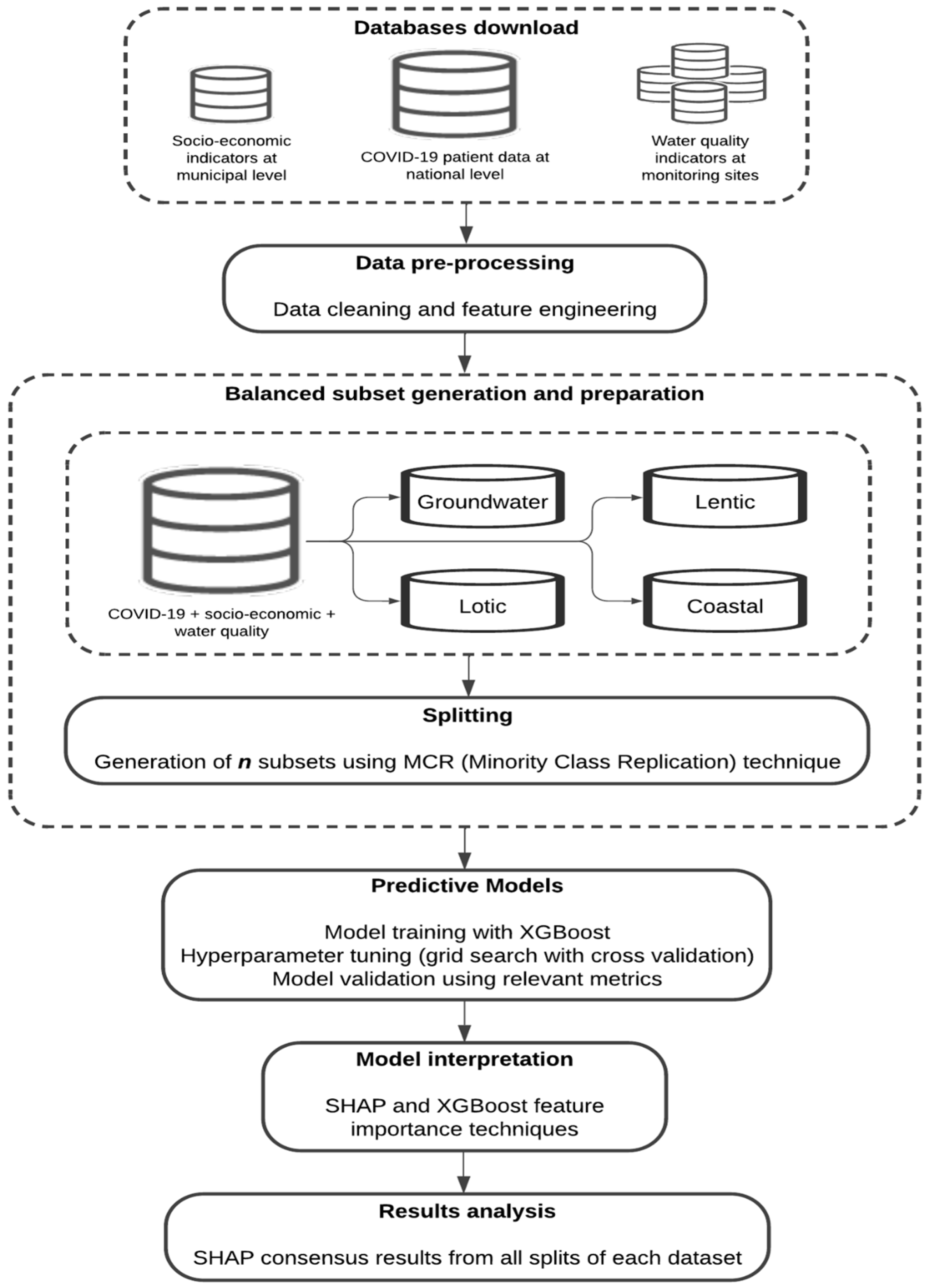
- COVID-19 database. This database, containing all confirmed, suspected, negative, and death cases, was downloaded from the Mexican government website [16].
- (b)
- Socioeconomic indicators. Municipal-level Human Development Index (HDI), and health (HS) and income (IS) subindexes, reported by the United Nations Development Programme [17] and collected by the National Council for Social Development Policy Evaluation [18], were assigned to each patient according to their municipality of residence. The most recent socioeconomic data from 2020 were used, as these are reported every 5 years. Four levels were defined for each variable, ranging from 0 to 1: very high (0.800–1.000), high (0.700–0.799), medium (0.551–0.699), and low (0.000–0.550). These indices were added as additional patient characteristics to analyze the impact of socioeconomic vulnerability on COVID-19 mortality, considering that impoverished populations often face greater health risks than those with better economic opportunities [19].
- (c)
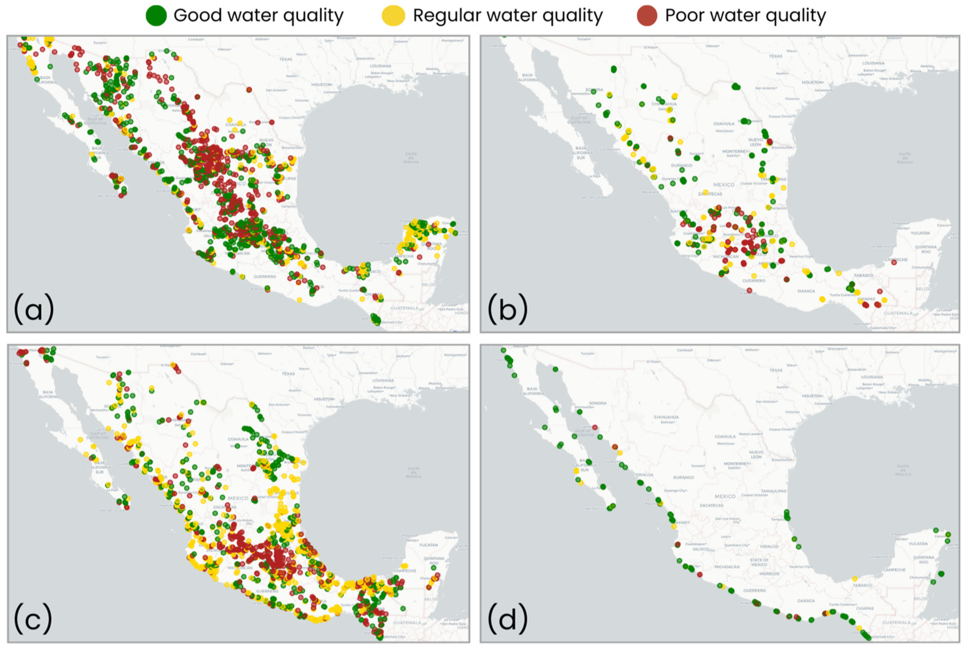
- Water quality parameters. The National Water Commission database [20] reports various contaminants and classifies water as good, regular, or poor at monitoring sites for four water body types: groundwater, lentic, lotic, and coastal (Table A1; [21]). The most recent data from 2018 to 2022 were used. Water quality classification was assigned as follows: (i) Groundwater: Regular quality indicates non-compliance with permitted levels for any of the following contaminants: alkalinity (Alk), conductivity (Cond), hardness (Hard), total dissolved solids (TDS), iron (Fe), or manganese (Mn). Poor quality indicates non-compliance for fluorides (F), fecal coliforms (FC), nitrate-nitrogen, or heavy metals such as arsenic (As), cadmium (Cd), chromium (Cr), mercury (Hg), and lead (Pb). (ii) Surface (lentic, lotic, and coastal) water: Regular quality indicates non-compliance for total suspended solids (TSS), FC, Escherichia coli (ECOLI), or percent oxygen saturation (surface ODs, medium ODm, and background ODb levels). Poor quality indicates non-compliance for any of the following higher risk parameters: 5-day biochemical oxygen demand (BOD5), chemical oxygen demand (COD), fecal enterococci (FE), or toxicity (Daphnia Magna 48 h, Vibrio Fischeri 15 min). Finally, good water quality is defined by compliance with all physicochemical and microbiological contaminants (Table A1).
2.1.2. Data Cleaning and Imputation
- (i)
- COVID-19 data cleaning: Only confirmed positive cases between 19 February 2020, and 28 February 2023, were considered, totaling 13,494,572 cases, of which 990,542 were hospitalized and 436,138 deceased. The selected variables included: (i) comorbidities: diabetes, hypertension, obesity, cardiovascular disease, chronic kidney disease (CKD), smoking, chronic obstructive pulmonary disease (COPD), asthma, and immunosuppression); (ii) patient characteristics: sex, age, hospitalized or outpatient status, pneumonia, intubation, and intensive care unit (ICU) admission; (iii) medical units: IMSS (Mexican Social Security Institute), ISSSTE (Institute of Social Security and Services for State Workers), SSA (Secretariat of Health), military, private, and other; and (iv) outcome variable: patient survival status (alive or dead). Cases with missing values in any of the selected variables were excluded from the analysis.
- (ii)
- Socioeconomic data imputation: For 570 municipalities in Oaxaca, socioeconomic indicators (HDI, HS, and IS) are reported by region [18]. Therefore, the state average was assigned to these municipalities.
- (iii)
- Water quality data imputation: Due to missing values across multiple municipalities, a state-label imputation was applied separately for each water body type. For states with >30% missing data, values were imputed based on geographic proximity by copying data from neighboring municipalities. For states with ≤30% missing data, the proportion of water quality ratings was calculated at the state level, and missing values were assigned randomly while maintaining the original distribution.
2.1.3. Feature Engineering
2.1.4. Integration of COVID-19 and Water Quality Databases
2.1.5. Demographic and Clinical Features Description Across Datasets
2.1.6. Balanced Subsets Generation and Preparation
2.2. XGBoost Models Training
Hyperparameter Tuning and Cross-Validation
- max_depth: Maximum tree depth (default = 6; range: [0, ∞]; values evaluated: [3–10]).
- min_child_weight: Minimum sum of instance weights in a child node (default = 1, range = [0, ∞]; values: [3–6]).
- gamma: Minimum loss reduction to create a partition (default = 0, range = [0, ∞]; values: [0–0.5 in increments of 0.1]).
- subsample: Fraction of training samples per tree (default = 1, range = [0, 1]; values: [0.1–1.0 in increments of 0.1]).
- colsample_bytree: Fraction of features used per tree (default = 1, range = [0, 1]; values [0.2–1.0 in increments of 0.1]).
- reg_lambda: L2 regularization on weights (default = 1, range = [0, ∞]; values: [0.3–1.0 in increments of 0.1]).
- n_estimators: Number of boosting iterations (default = 100, range = [1, ∞]; values: [50, 100, 150]).
2.3. XGBoost Model Evaluation
2.4. XGBoost Model Interpretation with SHAP
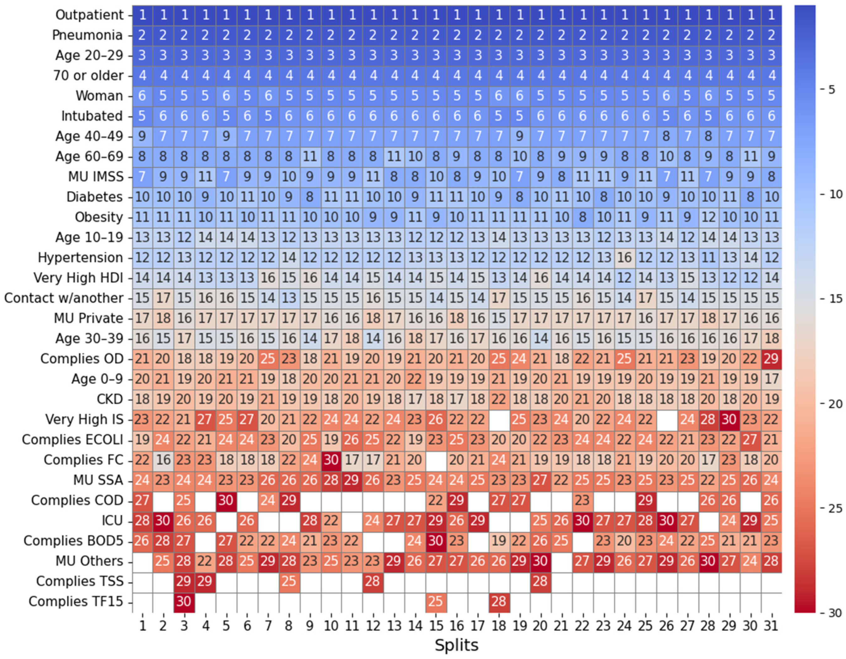
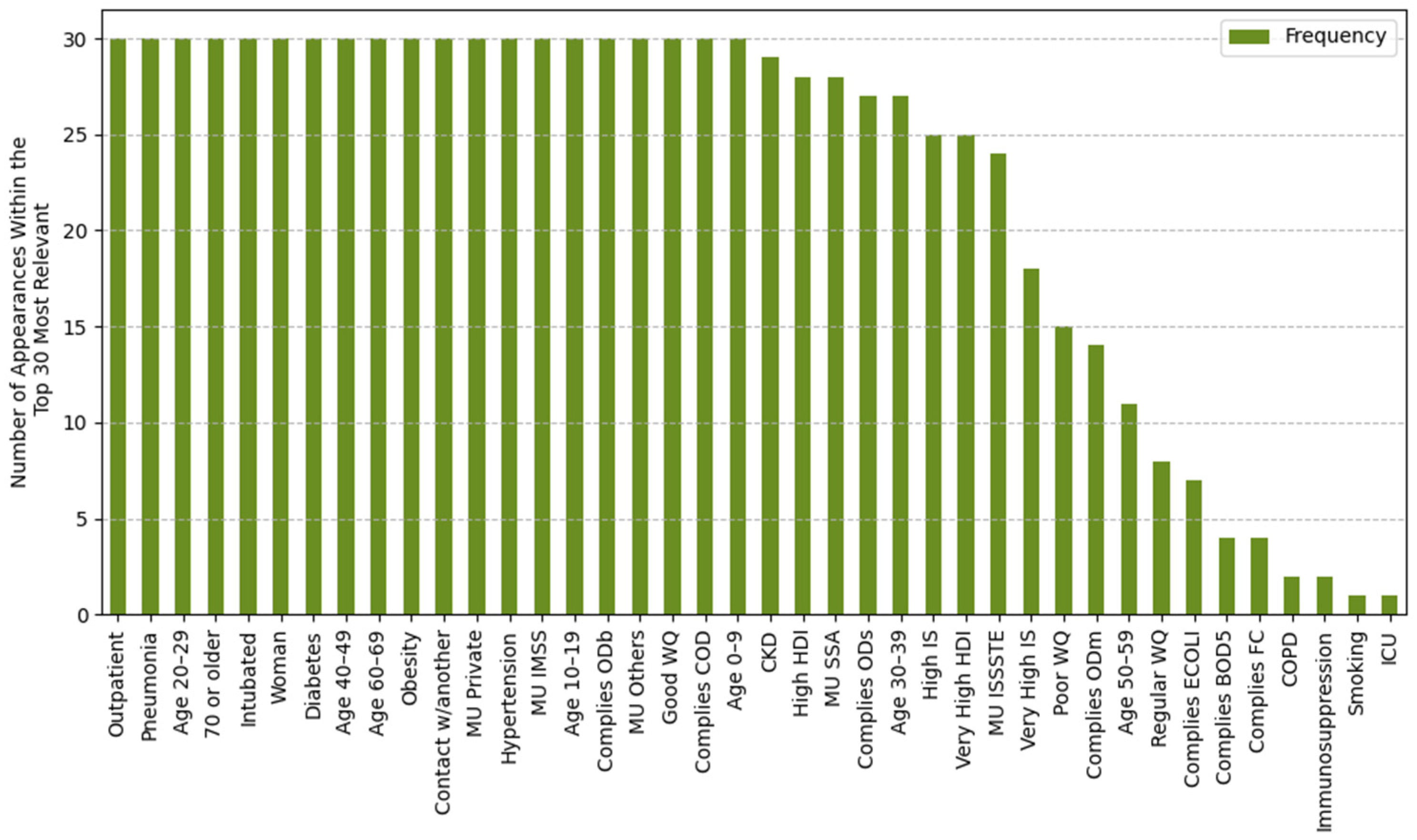
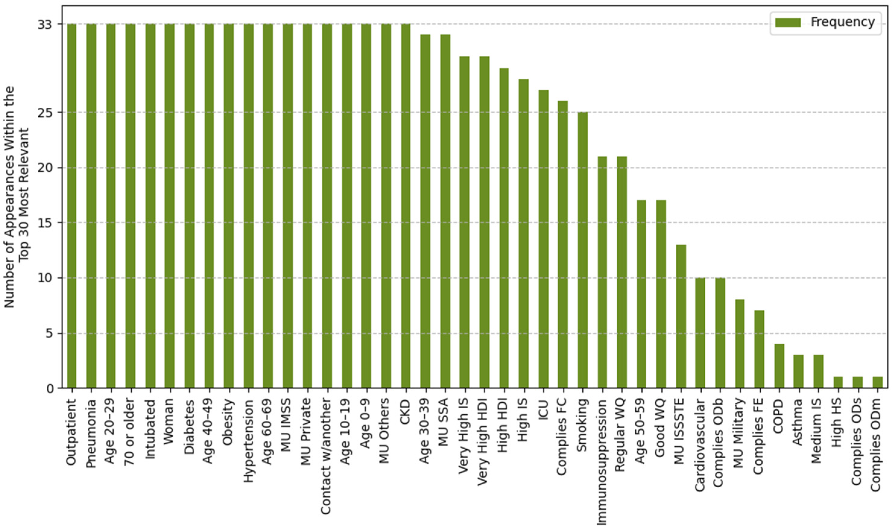
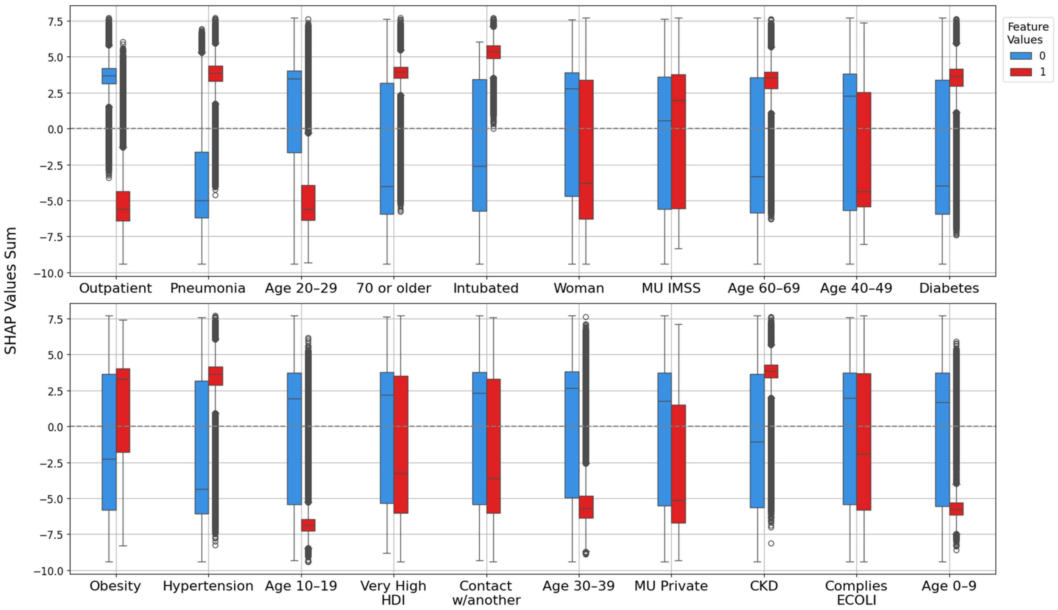
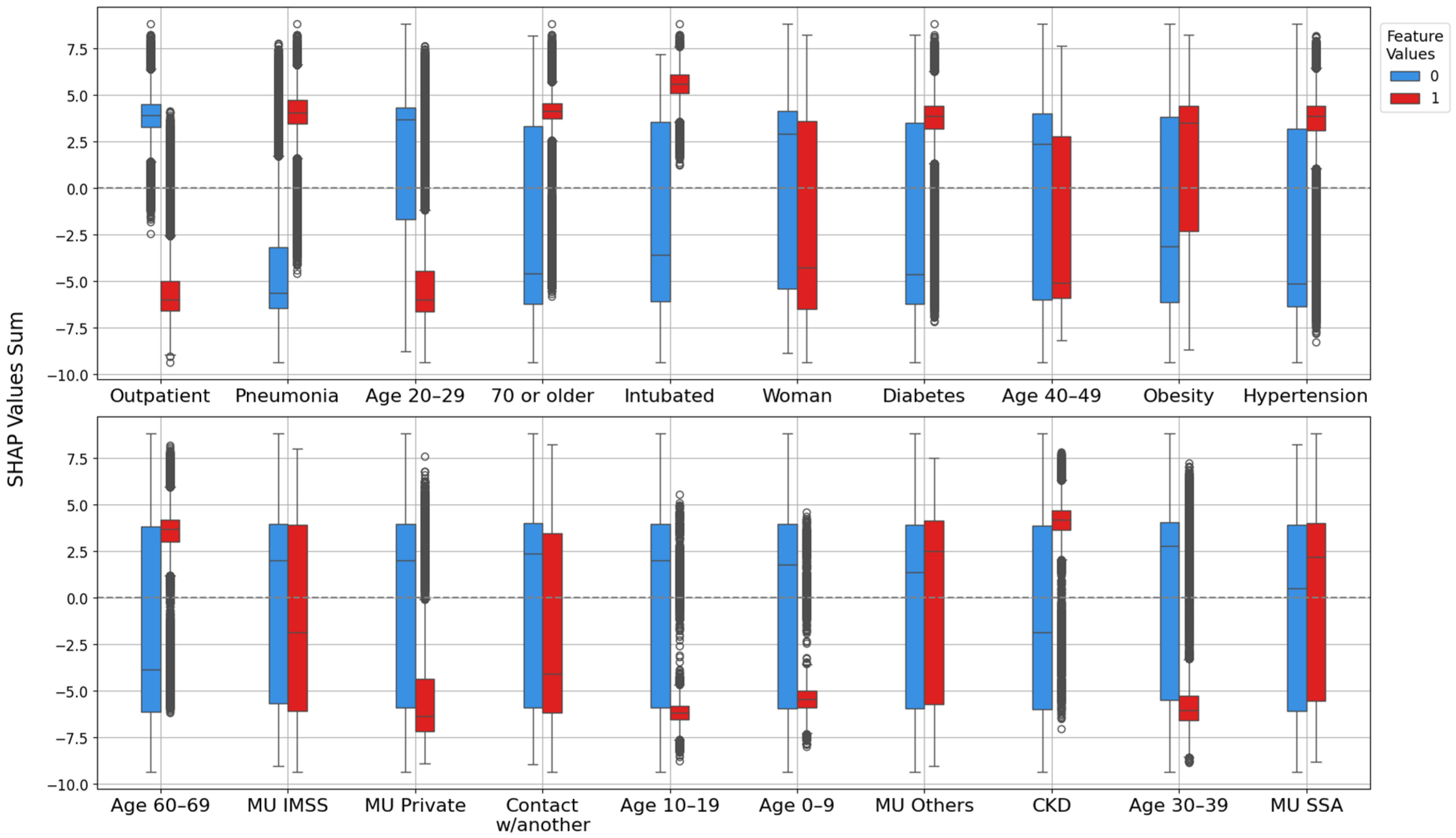
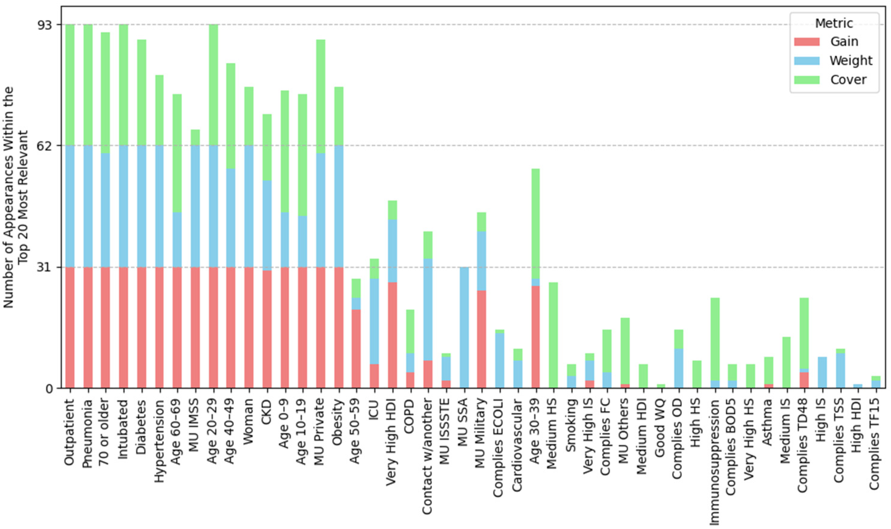
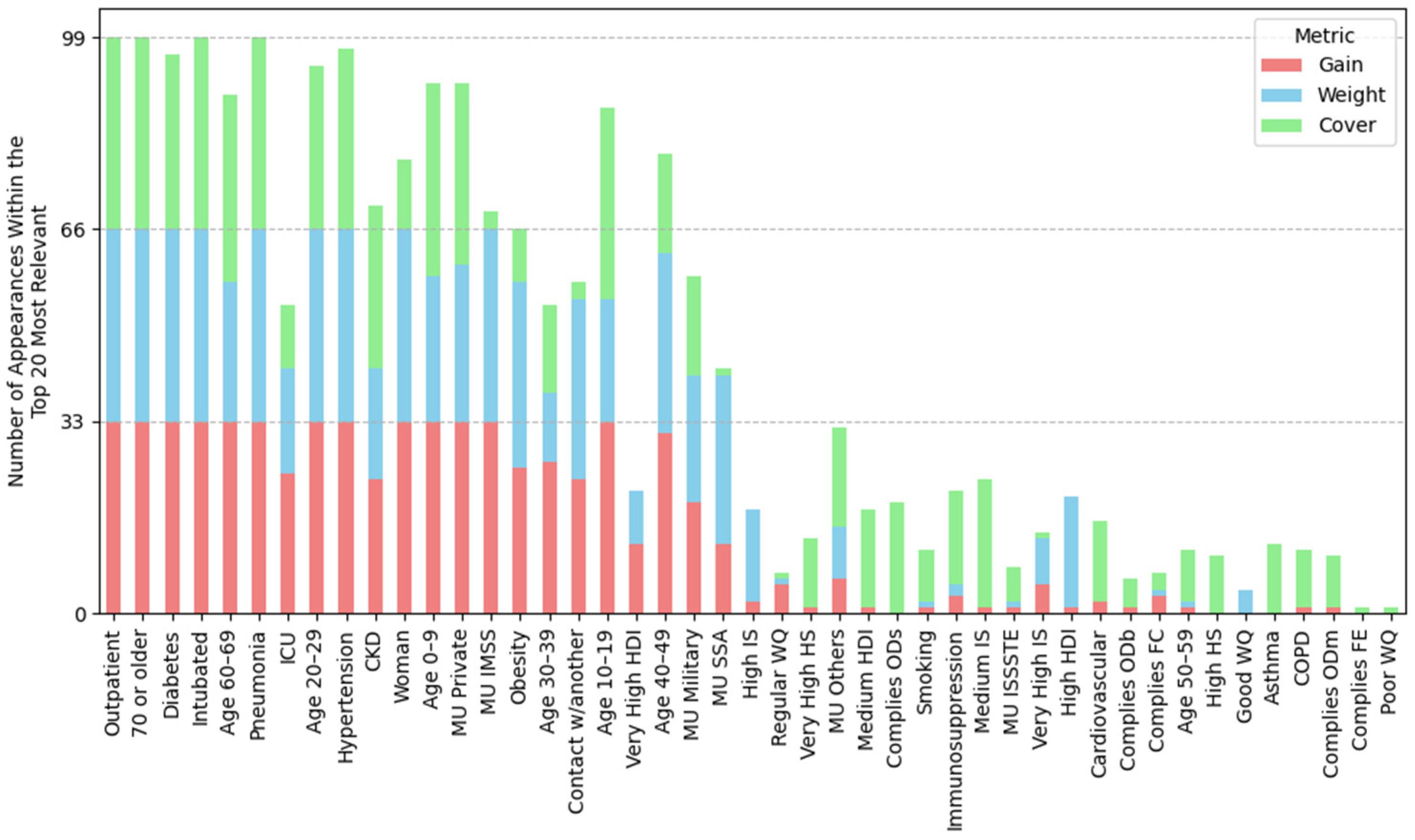
2.4.1. Feature Importance Based on Top 30 SHAP Rankings Across All Splits
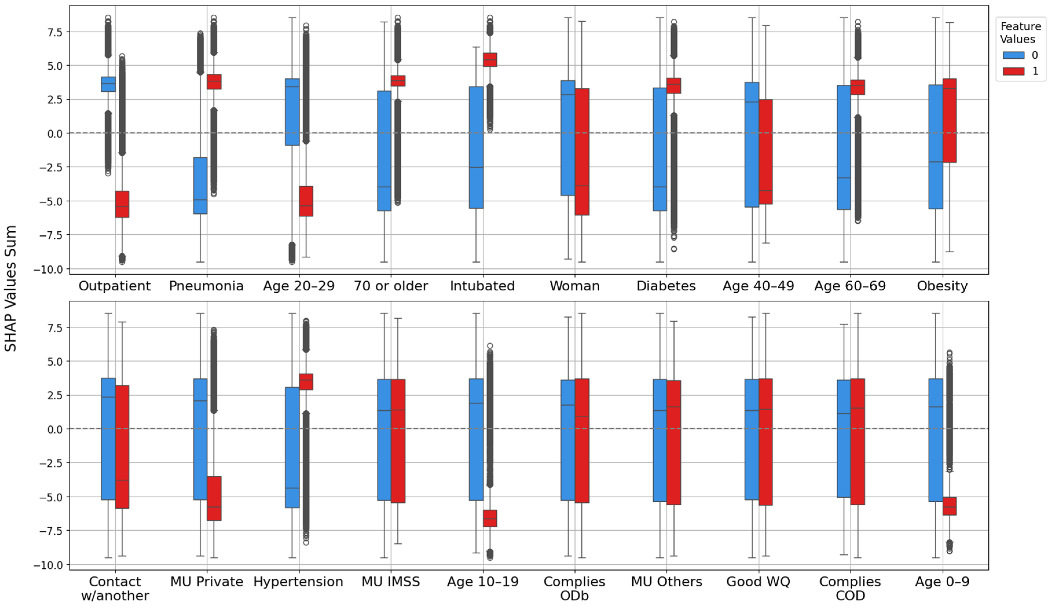
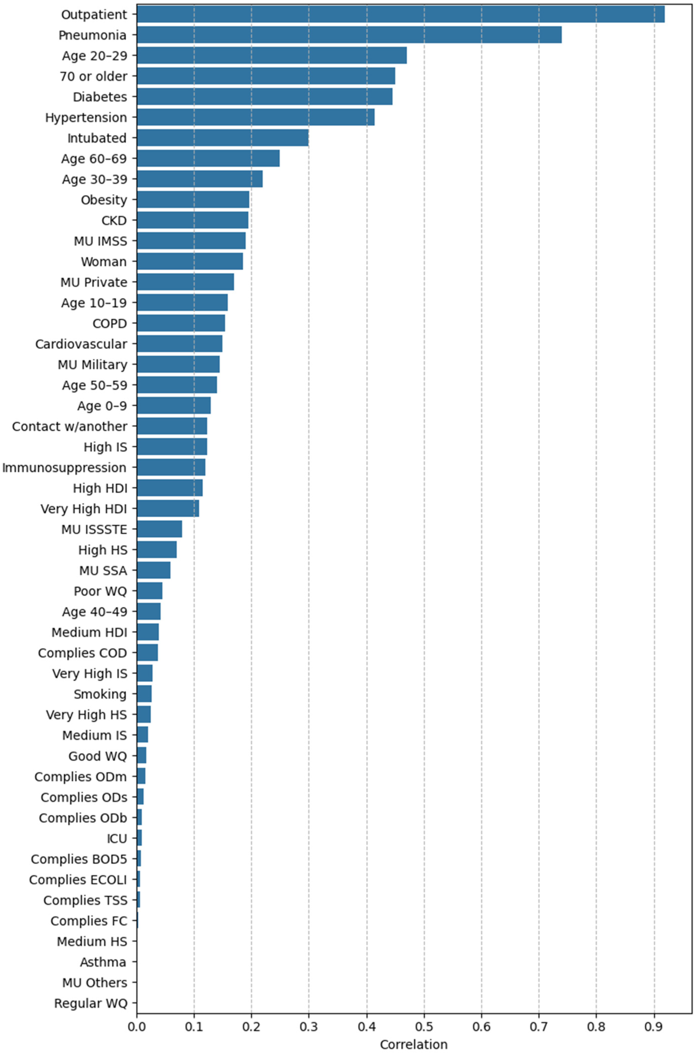
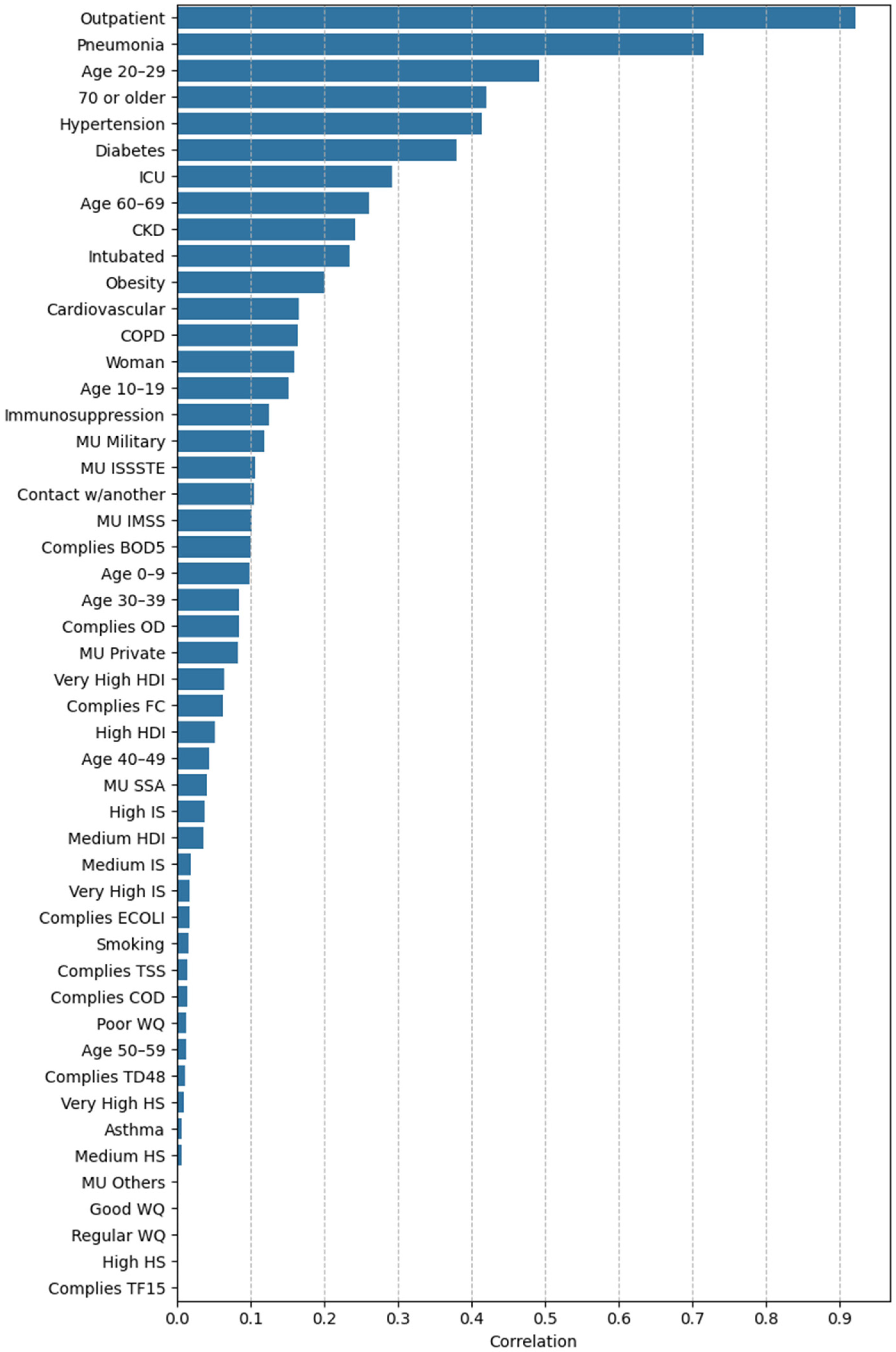
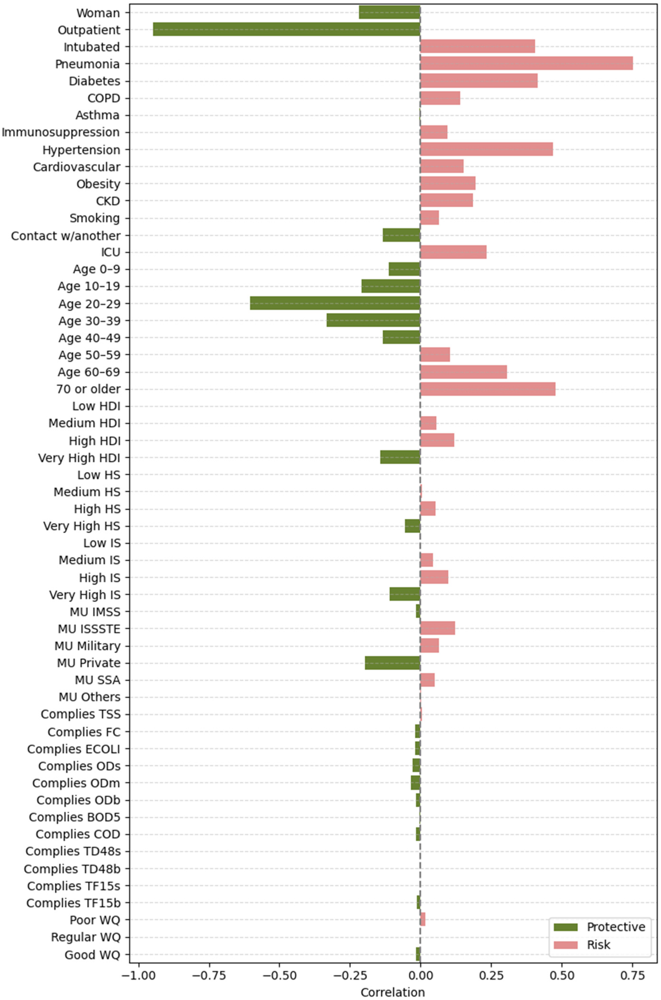
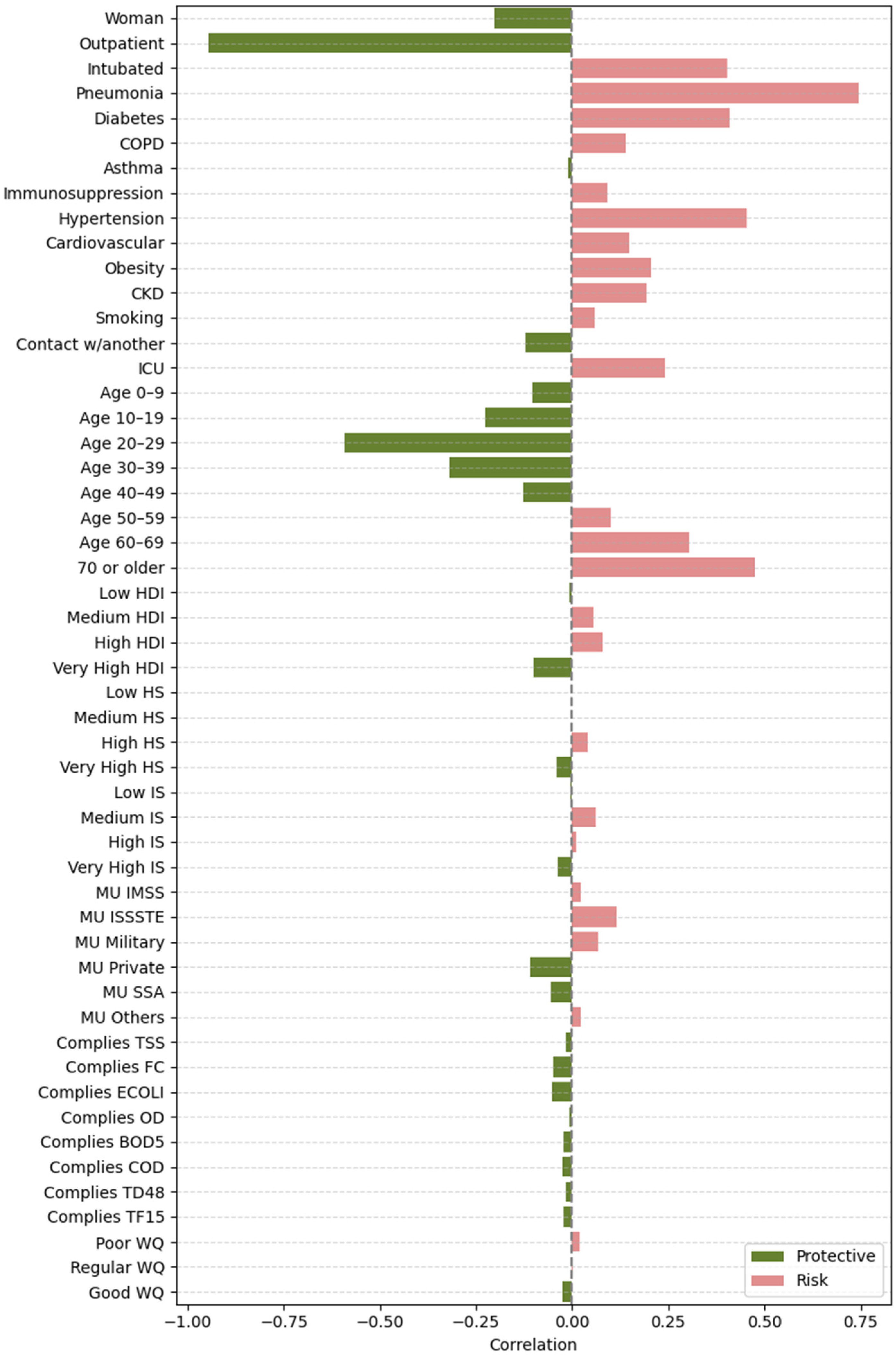
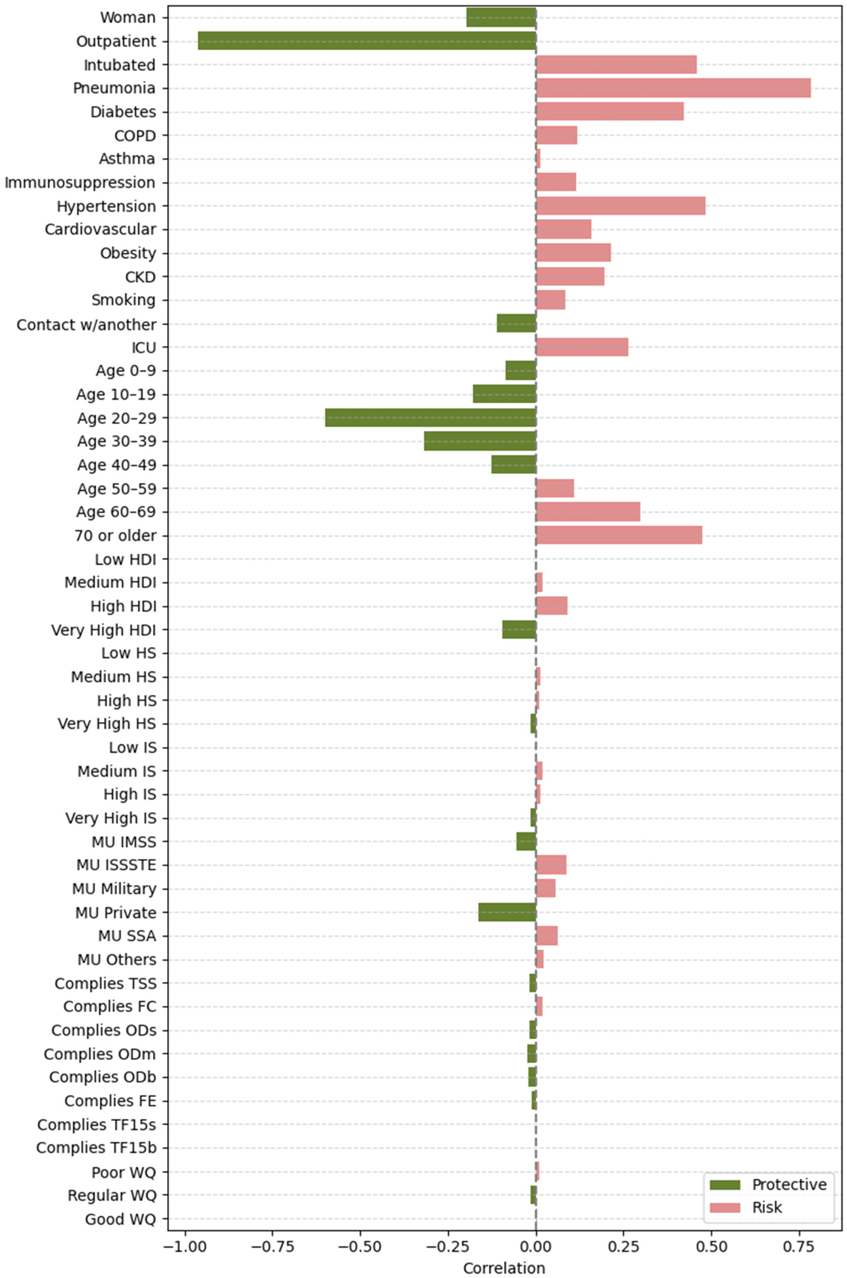
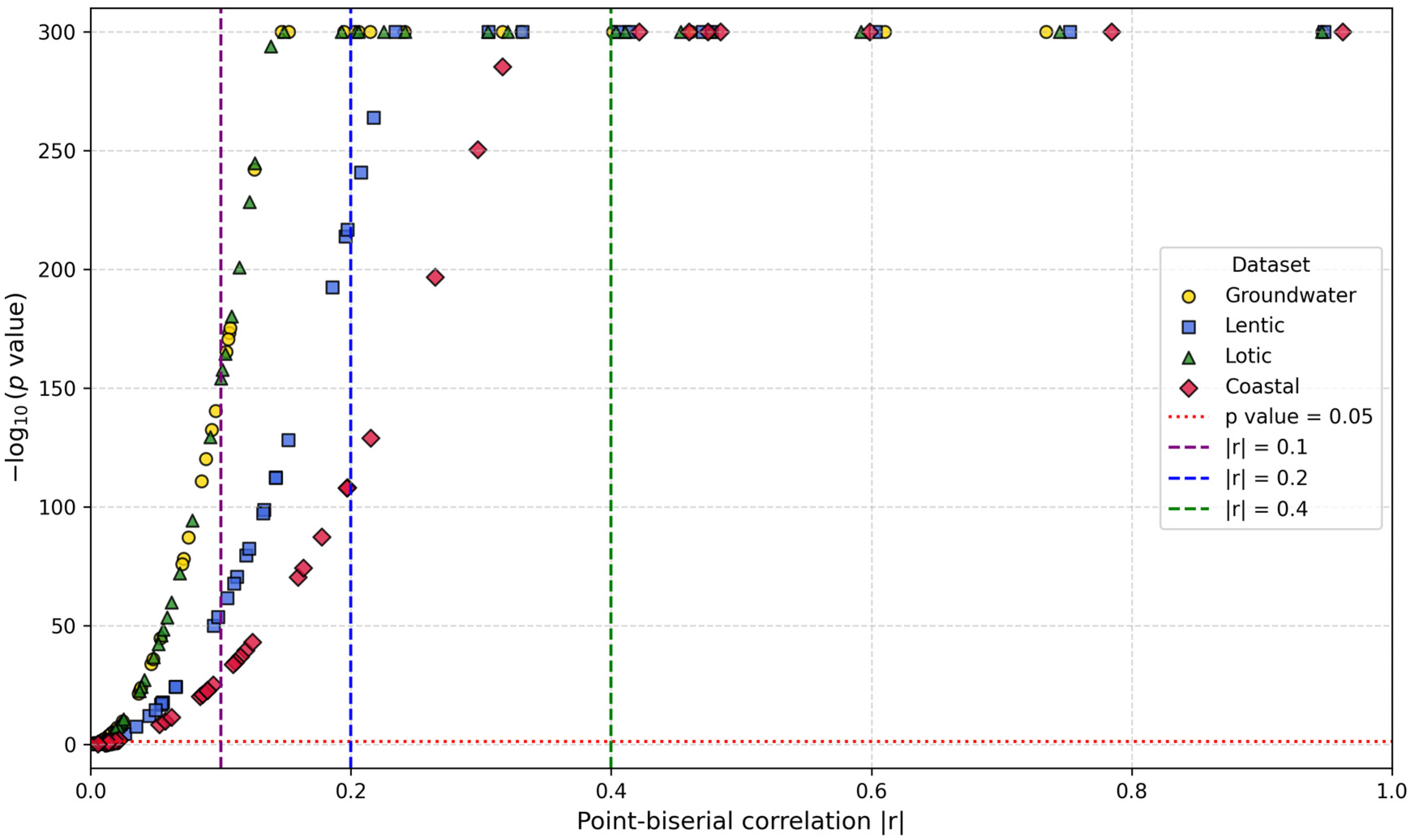
2.4.2. Feature Importance Based on Point-Biserial Correlation Across All Splits
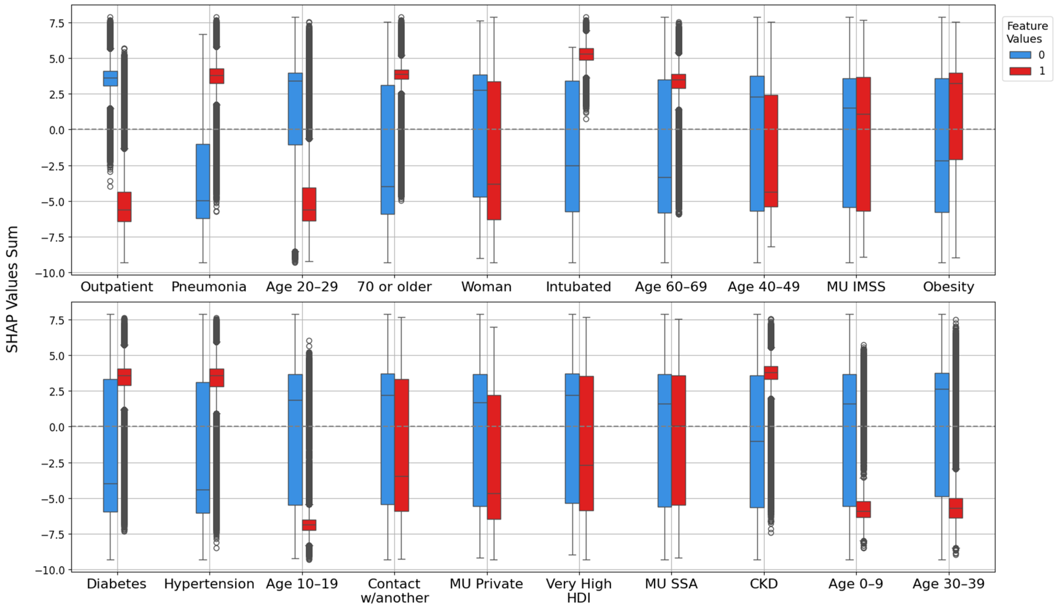
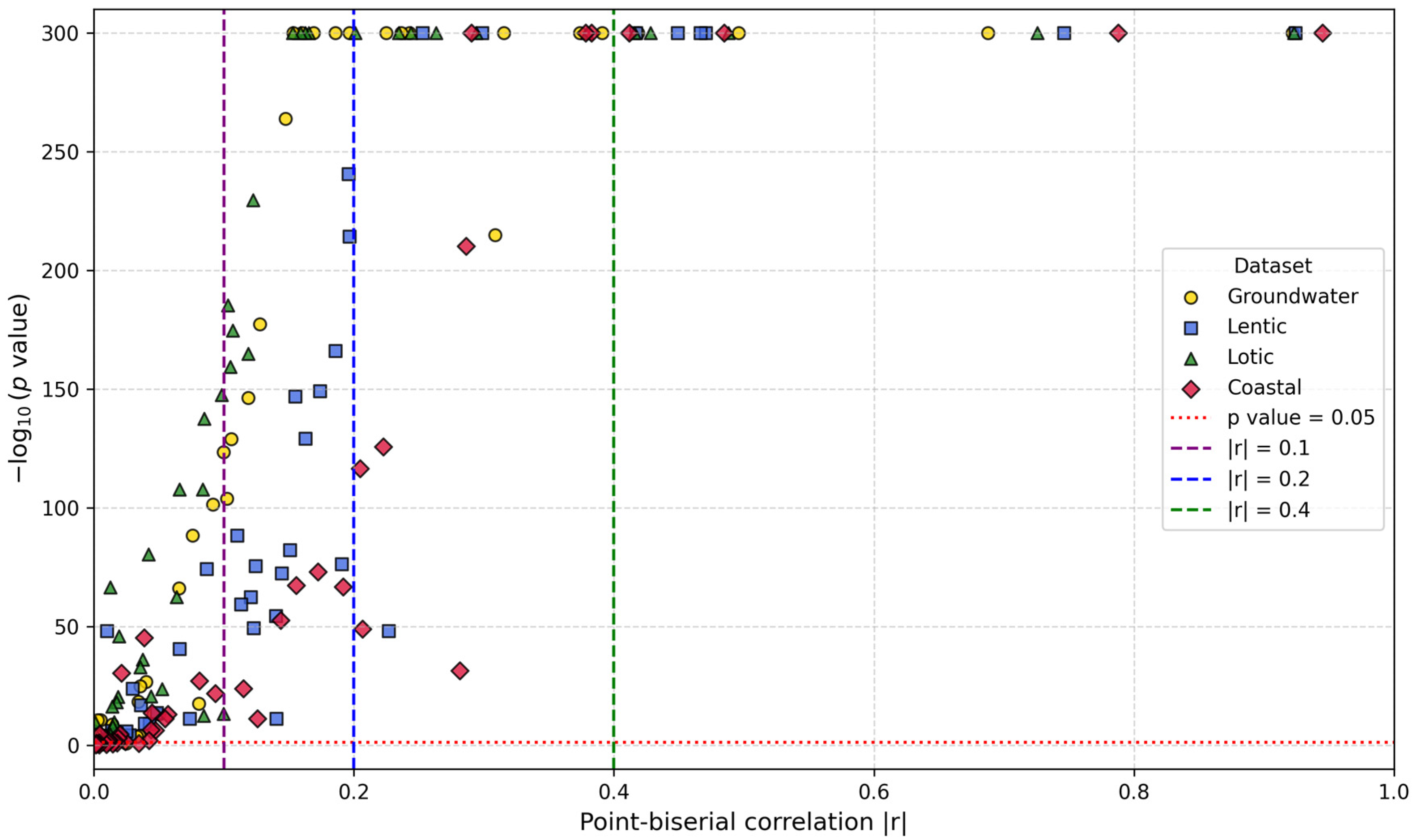
- SHAP vs. target: Correlation between each feature’s SHAP values and patient outcomes. This analysis highlights whether higher SHAP values for a feature are associated with increased or decreased mortality risk.
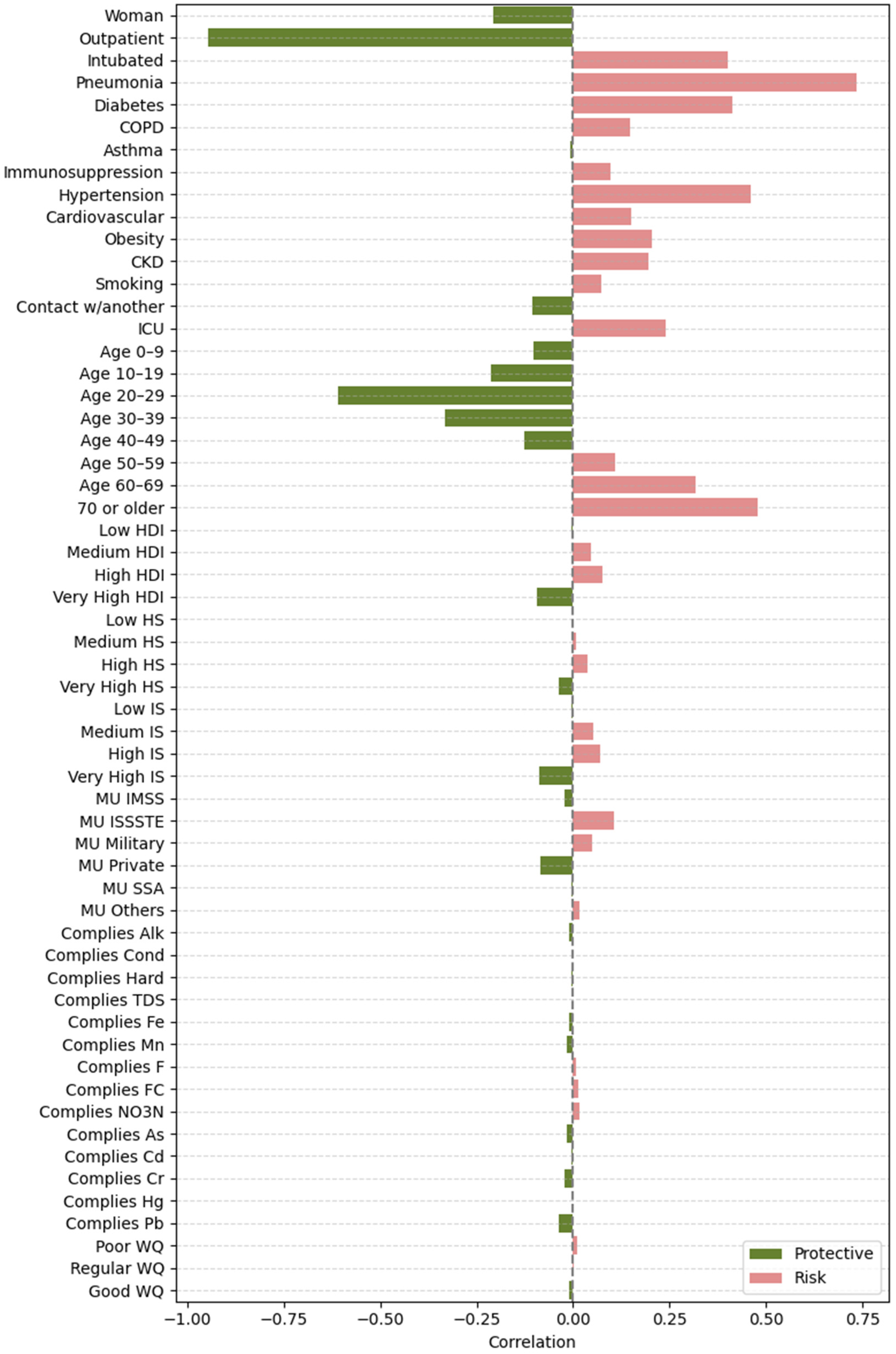
- Feature vs. SHAP: Correlation between binary feature values and the aggregated SHAP values: individual SHAP values provided a weighted measure of feature importance. Positive correlations indicated risk factors; negative correlations indicated protective factors.
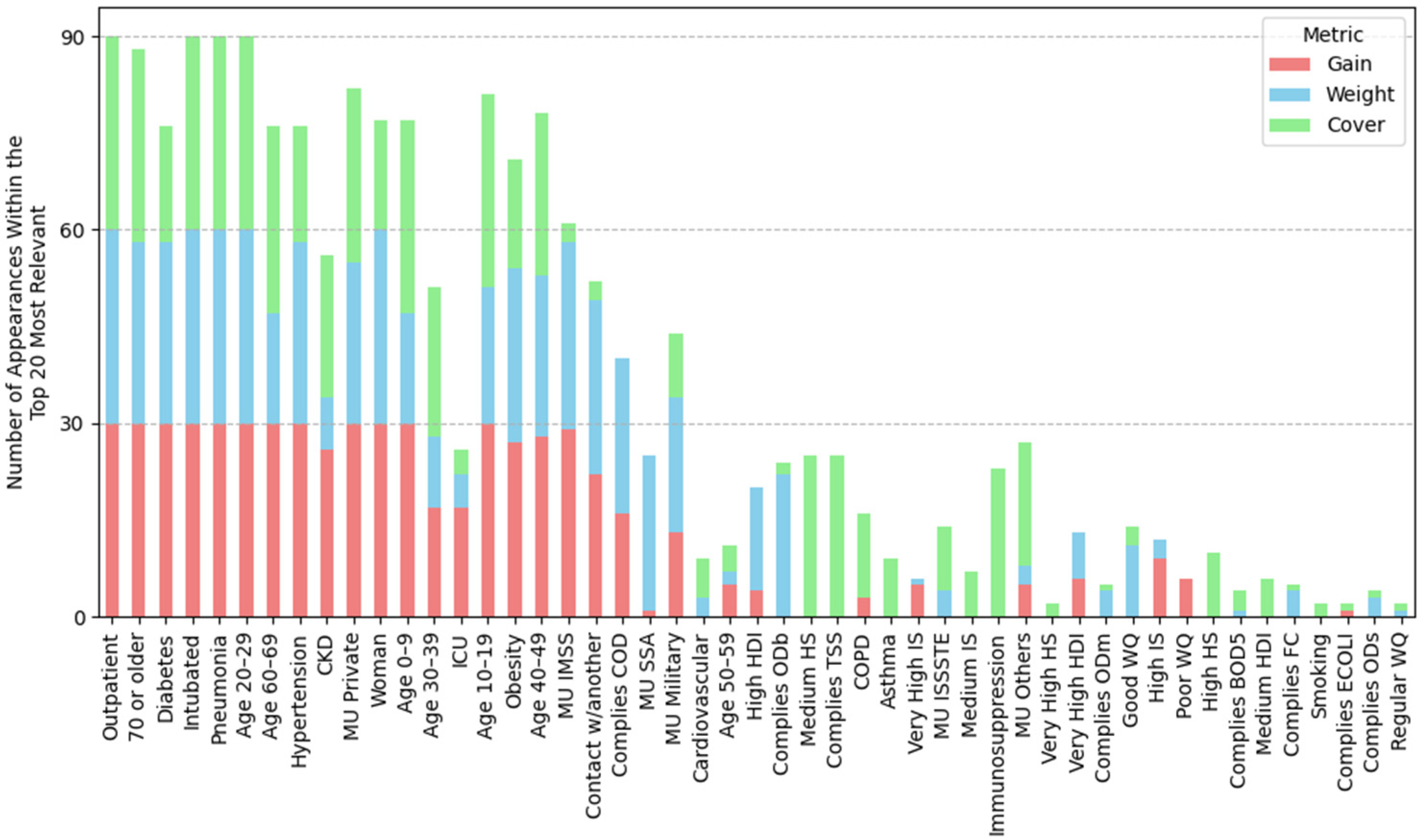
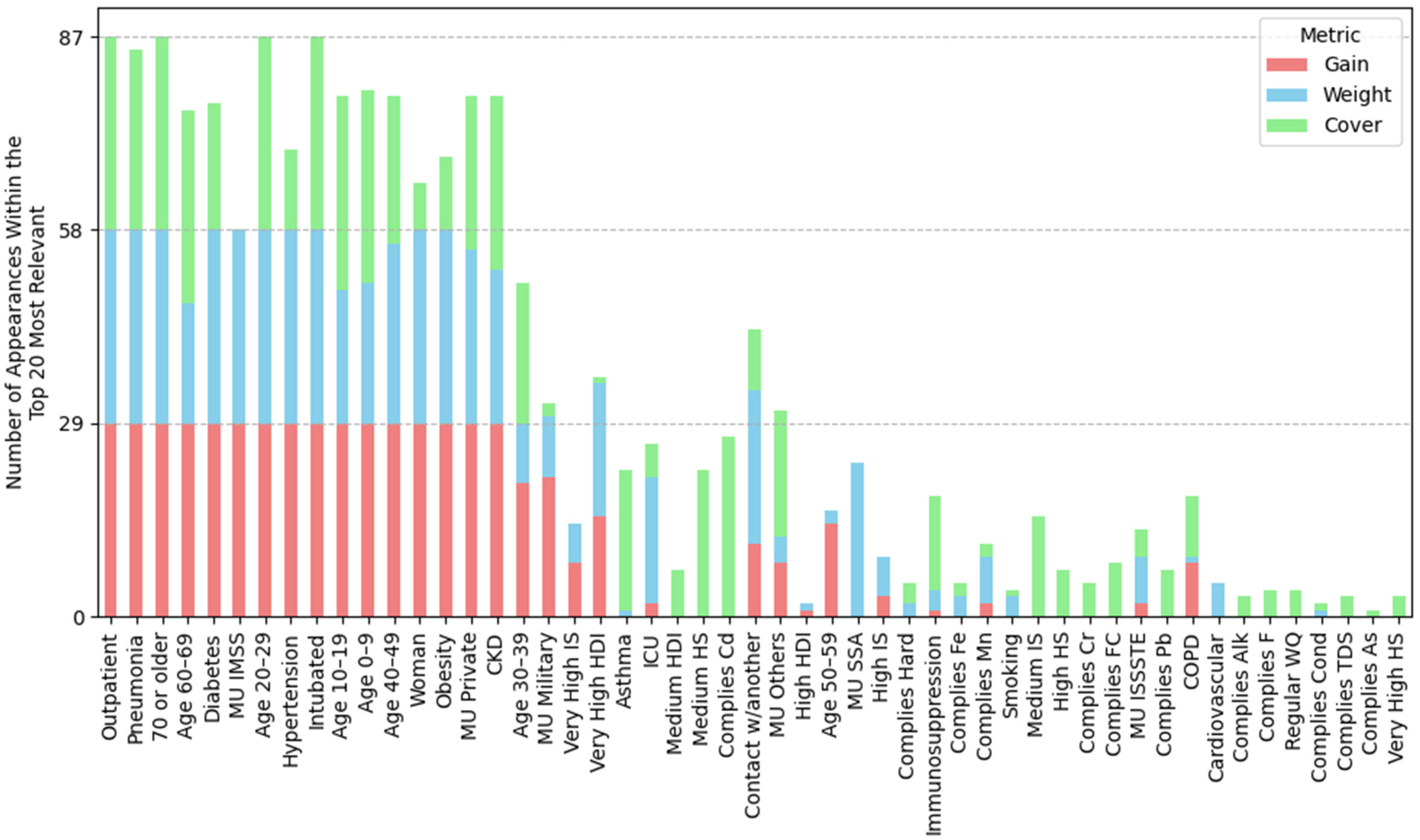
2.5. XGBoost Models Interpretation Using Tree-Related Metrics
3. Results
3.1. XGBoost Model Performance
- Groundwater: The F1 Score values were 0.971 (±5.0 × 10⁻⁴) for training and 0.970 (±1.1 × 10⁻³) for testing. MCC values were 0.942 (±1.0 × 10⁻³) and 0.940 (±2.2 × 10⁻³), respectively.
- Lentic: The F1 Score values were 0.973 (±3.0 × 10⁻⁴) for training and 0.972 (±5.0 × 10⁻⁴) for testing. MCC values were 0.946 (±5.0 × 10⁻⁴) and 0.944 (±1.0 × 10⁻³), respectively.
- Lotic: The F1 Score values were 0.972 (±3.0 × 10⁻⁴) for training and 0.972 (±3.0 × 10⁻⁴) for testing. MCC values were 0.944 (±6.0 × 10⁻⁴) and 0.943 (±8.0 × 10⁻⁴).
- Coastal: The F1 Score values were 0.979 (±3.0 × 10⁻⁴) for training and 0.978 (±4.0 × 10⁻⁴) for testing. MCC values were 0.958 (±6.0 × 10⁻⁴) and 0.956 (±8.0 × 10⁻⁴).
| Metric | Groundwater | Lentic | Lotic | Coastal |
|---|---|---|---|---|
| (A) Mean (standard deviation) performance metrics for XGBoost models across different datasets: | ||||
| Training accuracy | 0.971 5.16 × 10⁻⁴ | 0.973 2.78 × 10⁻⁴ | 0.972 3.21 × 10⁻⁴ | 0.979 3.21 × 10⁻⁴ |
| Testing accuracy | 0.970 1.143 × 10⁻³ | 0.972 5.08 × 10⁻⁴ | 0.972 3.16 × 10⁻⁴ | 0.978 3.94 × 10⁻⁴ |
| Training precision | 0.968 8.99 × 10⁻⁴ | 0.970 4.68 × 10⁻⁴ | 0.969 4.35 × 10⁻⁴ | 0.973 4.98 × 10⁻⁴ |
| Testing precision | 0.968 2.13 × 10⁻³ | 0.970 9.13 × 10⁻⁴ | 0.968 6.59 × 10⁻⁴ | 0.973 7.03 × 10⁻⁴ |
| Training recall | 0.974 3.65 × 10⁻⁴ | 0.976 1.94 × 10⁻⁴ | 0.976 3.44 × 10⁻⁴ | 0.985 3.12 × 10⁻⁴ |
| Testing recall | 0.972 6.77 × 10⁻⁴ | 0.975 2.82 × 10⁻⁴ | 0.975 2.05 × 10⁻⁴ | 0.983 2.48 × 10⁻⁴ |
| Training F1 score | 0.971 5.01 × 10⁻⁴ | 0.973 2.69 × 10⁻⁴ | 0.972 2.98 × 10⁻⁴ | 0.979 3.13 × 10⁻⁴ |
| Testing F1 score | 0.970 1.105 × 10⁻³ | 0.972 4.88 × 10⁻⁴ | 0.972 3.4 × 10⁻⁴ | 0.978 3.8 × 10⁻⁴ |
| Training MCC | 0.942 1.014 × 10⁻³ | 0.946 5.47 × 10⁻⁴ | 0.944 5.78 × 10⁻⁴ | 0.958 6.36 × 10⁻⁴ |
| Testing MCC | 0.940 2.237 × 10⁻³ | 0.944 9.94 × 10⁻⁴ | 0.943 8.02 × 10⁻⁴ | 0.956 7.73 × 10⁻⁴ |
| (B) Most frequently selected hyperparameter values for XGBoost models across different datasets: | ||||
| max_depth | 8 (37%), 4 (24%), 10 (17%) | 4 (33%), 3 (23%), 7 (16%) | 6 (25%), 9 (22%), 5 (22%) | 3 (74%), 4 (12%), 6 (6%) |
| mid_child_weight | 6 (41%), 5 (37%), 4 (10%) | 4 (33%), 3 (26%), 6 (23%) | 3 (35%), 6 (32%), 4 (22%) | 4 (42%), 5 (33%), 3 (12%) |
| gamma | 0.0 (37%), 0.1 (24%), 0.3 (13%) | 0.0 (33%), 0.2 (30%), 0.4 (13%) | 0.0 (38%), 0.1 (25%), 0.2 (22%) | 0.2 (33%), 0.5 (21%), 0.4 (15%) |
| colsample_bytree | 0.7 (37%), 1.0 (31%), 0.8 (13%) | 1.0 (36%), 0.4 (23%), 0.3 (13%) | 1.0 (45%), 0.6 (19%), 5 (16%) | 0.6 (24%), 0.3 (24%), 0.5 (21%) |
| subsample | 0.7 (82%), 1.0 (13%), 0.8 (3%) | 1.0 (70%), 0.8 (10%), 0.7 (10%) | 1.0 (64%), 0.9 (25%), 0.8 (6%) | 1.0 (63%), 0.9 (21%), 0.8 (6%) |
| n_estimators | 100 (75%), 50 (13%), 150 (10%) | 100 (83%), 150 (13%), 50 (3%) | 100 (90%), 150 (9%) | 100 (54%), 50 (27%), 150 (18%) |
| reg_lambda | 0.5 (55%), 0.4 (17%), 0.8 (10%) | 0.6 (43%), 1.0 (16%), 0.7 (13%) | 1.0 (51%), 0.9 (12%), 0.5 (12%) | 1.0 (42%), 0.9 (15%), 0.4 (12%) |
3.2. Model Explanation with SHAP Values
3.2.1. Feature Importance Analysis via SHAP Rankings Across All Splits
3.2.2. Feature Importance via Point-Biserial Correlation Across All Splits
3.3. Feature Importance via XGBoost Tree-Related Metrics
3.4. Condensed Analysis of Feature Importance Across All Datasets
3.4.1. Feature Importance by Position Rank
3.4.2. Water Quality and Socioeconomic Feature Importance
4. Discussion
4.1. Clinical and Demographic Factors
4.2. Environmental Factors
4.3. Socioeconomic Factors
4.4. Feature Importance Methodologies: A Comparative Analysis
4.5. Complementary Analysis: Evaluating Pre-Infection Predictors by Excluding Clinical Outcome Variables
5. Conclusions
Author Contributions
Funding
Data Availability Statement
Acknowledgments
Conflicts of Interest
Appendix A
| Pollutant Parameter | Units | Limits for Good Water Quality | Water Quality Classification for Non-Compliance |
|---|---|---|---|
| (a) Groundwater | |||
| Alkalinity (Alk) | mg CaCO3/L | 20 ≤ Alk ≤ 400 | Regular |
| Electrical conductivity (Cond) | μS/cm | Cond ≤ 2000 | Regular |
| Total hardness (Hard) | mg CaCO3/L | Hard ≤ 500 | Regular |
| Total dissolved solids (TDS) | mg/L | TDS ≤ 2000 | Regular |
| Iron (Fe) | mg/L | Fe ≤ 0.30 | Regular |
| Manganese (Mn) | mg/L | Mn ≤ 0.15 | Regular |
| Fluorides (F) | mg/L | F < 1.5 | Poor |
| Fecal coliforms (FC) | NMP/100_mL | FC ≤ 1000 | Poor |
| Nitrate-nitrogen (NO3-N) | mg/L | NO3-N ≤ 11 | Poor |
| Arsenic (As) | mg/L | As ≤ 0.025 | Poor |
| Cadmium (Cd) | mg/L | Cd ≤ 0.005 | Poor |
| Chromium (Cr) | mg/L | Cr ≤ 0.05 | Poor |
| Mercury (Hg) | mg/L | Hg ≤ 0.006 | Poor |
| Lead (Pb) | mg/L | Pb ≤ 0.01 | Poor |
| (b) Lotic water | |||
| Total suspended solids (TSS) | mg/L | TSS ≤ 150 | Regular |
| Fecal coliforms (FC) | NMP/100_mL | FC ≤ 1000 | Regular |
| Escherichia coli (ECOLI) | NMP/100 ml | ECOLI ≤ 850 | Regular |
| % oxygen demand saturation (OD%) | % Saturation | 30 < OD% ≤ 130 | Regular |
| 5-day biochemical oxygen demand (BOD5) | mg/L | BOD5 ≤ 30 | Poor |
| Chemical oxygen demand (COD) | mg/L | COD ≤ 40 | Poor |
| Toxicity Daphnia Magna, 48 h (TD48) | UT | TD48 < 5 | Poor |
| Toxicity Vibrio Fischeri, 15 min (TF15) | UT | TF15 < 5 | Poor |
| (c) Lentic water | |||
| Total suspended solids (TSS) | mg/L | TSS ≤ 150 | Regular |
| Fecal coliforms (FC) | NMP/100_mL | FC ≤ 1000 | Regular |
| Escherichia soli (ECOLI) | NMP/100 ml | ECOLI ≤ 850 | Regular |
| % OD at surface (ODs%) | % Saturation | 30 < ODs% ≤ 130 | Regular |
| % OD at medium (ODm%) | % Saturation | 30 < ODm% ≤ 130 | Regular |
| % OD at background (ODb%) | % Saturation | 30 < ODb% ≤ 130 | Regular |
| BOD5 | mg/L | BOD5 ≤ 30 | Poor |
| Chemical oxygen demand (COD) | mg/L | COD > 40 | Poor |
| TD48 at surface (TD48s) | UT | TD48s < 5 | Poor |
| TD48 at background (TD48b) | UT | TD48b < 5 | Poor |
| TF15 at surface (TF15s) | UT | TF15s < 5 | Poor |
| TF15 at background (TF15b) | UT | TF15b < 5 | Poor |
| (d) Coastal water | |||
| Total suspended solids (TSS) | mg/L | TSS ≤ 150 | Regular |
| Fecal coliforms (FC) | NMP/100_mL | FC ≤ 1000 | Regular |
| % OD at surface (ODs%) | % Saturation | 30 < ODs% ≤ 130 | Regular |
| % OD at medium (ODm%) | % Saturation | 30 > ODm% ≤ 130 | Regular |
| % OD at background (ODb%) | % Saturation | 30 > ODb% ≤ 130 | Regular |
| Fecal enterococci (FE) | NMP/100 ml | FE ≤ 200 | Poor |
| TF15 at surface (TF15s) | UT | TF15s < 5 | Poor |
| TF15 at background (TF15b) | UT | TF15b < 5 | Poor |




References
- PAHO. WHO Characterizes COVID-19 as a Pandemic. Available online: https://www.paho.org/en/news/11-3-2020-who-characterizes-covid-19-pandemic (accessed on 25 April 2025).
- WHO. WHO Coronavirus (COVID-19) Dashboard. Available online: https://covid19.who.int/ (accessed on 25 April 2025).
- Wollenstein-Betech, S.; Cassandras, C.G.; Paschalidis, I.C. Personalized predictive models for symptomatic COVID-19 patients using basic preconditions: Hospitalizations, mortality, and the need for an ICU or ventilator. Int. J. Med. Inform. 2020, 142, 104258. [Google Scholar] [CrossRef] [PubMed]
- Khadem, H.; Nemat, H.; Eissa, M.R.; Elliott, J.; Benaissa, M. COVID-19 mortality risk assessments for individuals with and without diabetes mellitus: Machine learning models integrated with interpretation framework. Comput. Biol. Med. 2022, 144, 105361. [Google Scholar] [CrossRef] [PubMed]
- Barría-Sandoval, C.; Ferreira, G.; Espinoza Venegas, M.; Marchant, V. Interpretable machine learning for mortality modeling on patients with chronic diseases considering the COVID-19 pandemic in a region of Chile: A Shapley value based approach. Res. Stat. 2023, 1, 2240334. [Google Scholar] [CrossRef]
- Datta, D.; George Dalmida, S.; Martinez, L.; Newman, D.; Hashemi, J.; Khoshgoftaar, T.M.; Shorten, C.; Sareli, C.; Eckardt, P. Using machine learning to identify patient characteristics to predict mortality of in-patients with COVID-19 in south Florida. Front. Digit. Health 2023, 5, 1193467. [Google Scholar] [CrossRef] [PubMed]
- Rojas-García, M.; Vázquez, B.; Torres-Poveda, K.; Madrid-Marina, V. Lethality risk markers by sex and age-group for COVID-19 in Mexico: A cross-sectional study based on machine learning approach. BMC Infect. Dis. 2023, 23, 18. [Google Scholar] [CrossRef] [PubMed]
- Li, H.; Ashrafi, N.; Kang, C.; Zhao, G.; Chen, Y.; Pishgar, M. A machine learning-based prediction of hospital mortality in mechanically ventilated ICU patients. PLoS ONE 2024, 19, e0309383. [Google Scholar] [CrossRef] [PubMed]
- Sharifi-Kia, A.; Nahvijou, A.; Sheikhtaheri, A. Machine learning-based mortality prediction models for smoker COVID-19 patients. BMC Med. Inform. Decis. Mak. 2023, 23, 129. [Google Scholar] [CrossRef] [PubMed]
- Casillas, N.; Ramón, A.; Torres, A.M.; Blasco, P.; Mateo, J. Predictive model for mortality in severe COVID-19 patients across the six pandemic waves. Viruses 2023, 15, 2184. [Google Scholar] [CrossRef] [PubMed]
- Carvantes-Barrera, A.; Díaz-González, L.; Rosales-Rivera, M.; Chávez-Almazán, L.A. Risk factors associated with COVID-19 lethality: A machine learning approach using Mexico database. J. Med. Syst. 2023, 47, 90. [Google Scholar] [CrossRef] [PubMed]
- Zhou, C.; Wheelock, Å.M.; Zhang, C.; Ma, J.; Li, Z.; Liang, W.; Gao, J.; Xu, L. Country-specific determinants for COVID-19 case fatality rate and response strategies from a global perspective: An interpretable machine learning framework. Popul. Health Metr. 2024, 22, 10. [Google Scholar] [CrossRef] [PubMed]
- Chu, L.; Nelen, J.; Crivellari, A.; Masiliūnas, D.; Hein, C.; Lofi, C. Relationships between geo-spatial features and COVID-19. hospitalisations revealed by machine learning models and SHAP values. Int. J. Digit. Earth 2024, 17, 2358851. [Google Scholar] [CrossRef]
- Effrosynidis, D.; Arampatzis, A. An evaluation of feature selection methods for environmental data. Ecol. Inform. 2021, 61, 101224. [Google Scholar] [CrossRef]
- Chawla, N.V.; Bowyer, K.W.; Hall, L.O.; Kegelmeyer, W.P. SMOTE: Synthetic Minority Over-sampling Technique. J. Artif. Intell. Res. 2002, 16, 321–357. [Google Scholar] [CrossRef]
- National Epidemiological Surveillance System. Datos Abiertos-Bases Históricas-Dirección General de Epidemiología. Available online: https://www.gob.mx/salud/documentos/datos-abiertos-bases-historicas-direccion-general-de-epidemiologia (accessed on 4 November 2024).
- United Nations Development Programme. Índice de Desarrollo Humano (IDH) Municipal Resultados 2010–2020 [Dataset]. Available online: https://drive.google.com/drive/folders/1GRxyxSIPAL629vOnMLsLZgX70iqVo5ZX (accessed on 4 November 2024).
- United Nations Development Programme. Informe de Desarrollo Humano Municipal 2010–2020: Una Década de Transformaciones Locales en México. Programa de las Naciones Unidas para el Desarrollo, p. 99. Available online: https://www.undp.org/es/mexico/publicaciones/informe-de-desarrollo-humano-municipal-2010-2020-una-decada-de-transformaciones-locales-en-mexico-0 (accessed on 4 November 2024).
- Pérez-Tamayo, R. Patología de la Pobreza; Fondo de Cultura Económica: Mexico City, Mexico, 2016; p. 57. [Google Scholar]
- Comisión Nacional del Agua. Resultados de la Red Nacional de medición de Calidad del Agua (RENAMECA). Available online: https://www.gob.mx/conagua/articulos/resultados-de-la-red-nacional-de-medicion-de-calidad-del-agua-renameca?idiom=es (accessed on 11 February 2025).
- Díaz-González, L.; Aguilar-Rodríguez, R.A.; Pérez-Sansalvador, J.C.; Lakouari, N. AQuA-P: A machine learning-based tool for water quality assessment. J. Contam. Hydrol. 2025, 269, 104498. [Google Scholar] [CrossRef] [PubMed]
- Chen, T.; Guestrin, C. XGBoost: A scalable tree boosting system. In Proceedings of the ACM SIGKDD International Conference on Knowledge Discovery and Data Mining, San Francisco, CA, USA, 13–17 August 2016; pp. 785–794. [Google Scholar] [CrossRef]
- Russell, S.; Norvig, P. (Eds.) Decision Trees. In Artificial Intelligence: A Modern Approach, 4th ed.; Pearson: Boston, MA, USA, 2020; p. 1136. [Google Scholar]
- XGBoost Python Package. Available online: https://xgboost.readthedocs.io/en/stable/python/index.html (accessed on 11 June 2025).
- Anggoro, D.A.; Mukti, S.S. Performance Comparison of Grid Search and Random Search Methods for Hyperparameter Tuning in Extreme Gradient Boosting Algorithm to Predict Chronic Kidney Failure. Int. J. Intell. Eng. Syst. 2021, 14, 201. [Google Scholar] [CrossRef]
- XGBoost Contributors. XGBoost Parameters. Available online: https://xgboost.readthedocs.io/en/stable/parameter.html (accessed on 11 February 2025).
- Bishop, C.M. Pattern Recognition and Machine Learning; Springer: New York, NY, USA, 2006; p. 738. [Google Scholar]
- Lundberg, S.M.; Lee, S.I. A unified approach to interpreting model predictions. In Advances in Neural Information Processing Systems; Curran Associates, Inc.: Long Beach, CA, USA, 2017; Available online: https://arxiv.org/abs/1705.07874 (accessed on 11 June 2025).
- Shapley, L.S. A value for n-person games. In The Shapley Value; Thomson, R.E., Ed.; Cambridge University Press: Cambridge, UK, 2009; pp. 31–40. [Google Scholar] [CrossRef]
- Kornbrot, D. Point Biserial Correlation. In Wiley StatsRef: Statistics Reference Online; Wiley: Hoboken, NJ, USA, 2014. [Google Scholar] [CrossRef]
- Toribio-Colin, Y.S. Factors Associated with COVID-19 Mortality in Mexico: A Machine Learning Approach Using Clinical, Socioeconomic, and Environmental Data [Dataset]. Zenodo 2025. [Google Scholar] [CrossRef]
- Casini, F.; Roccetti, M. Reopening Italy’s schools in September 2020: A Bayesian estimation of the change in the growth rate of new SARS-CoV-2 cases. BMJ Open 2021, 11, e051458. [Google Scholar] [CrossRef] [PubMed]
- Gandini, S.; Rainisio, M.; Iannuzzo, M.L.; Bellerba, F.; Cecconi, F.; Scorrano, L. A cross-sectional and prospective cohort study of the role of schools in the SARS-CoV-2 second wave in Italy. Lancet Reg. Health Eur. 2021, 5, 100092. [Google Scholar] [CrossRef] [PubMed]


| Reference | Analysis Approach | Analysis Techniques | Identified Risk Factors |
|---|---|---|---|
| Wollenstein-Betech et al., 2020 [3] | Basic interpretable models | Logistic regression | Age, diabetes, renal failure, and immunosuppression are risk factors for hospitalization and mortality. |
| Khadem et al., 2022 [4] | Basic interpretable methods, ensemble models, and model explanation techniques | Random forest, SHAP, K-means | Neutrophil-lymphocyte ratio (NLR) and sodium are mortality risk factors in diabetic patients; estimated glomerular filtration rate (eGFR), albumin, and age in non-diabetic patients. |
| Barría-Sandoval et al., 2023 [5] | Ensemble models and model explanation techniques | XGBoost, SHAP, BorutaSHAP | Age and place of death as predictors of chronic disease and COVID-19 mortality. |
| Datta et al., 2023 [6] | Ensemble models and class-balancing techniques | Random forest, SMOTE | Age, diabetes, hypertension, and chronic kidney disease are risk factors for mortality. |
| Rojas-García et al., 2023 [7] | Ensemble models and model explanation techniques | XGBoost, SHAP | Diabetes and chronic kidney disease are risk factors in cases without intubation and ICU. |
| Li et al., 2024 [8] | Basic interpretable models, ensemble models, distance-based models, and class-balancing techniques | CatBoost, XGBoost, decision tree, random forest, SVMs, KNN, logistic regression, SMOTE | Age, vital signs, key laboratory values (bicarbonate, creatinine, electrolytes), specific disease counts, and comorbidities (e.g., organ failure, sepsis, hypertension, respiratory dysfunction). |
| Sharifi-Kia et al., 2023 [9] | Ensemble models, model explanation and class-balancing techniques | XGBoost, SMOTE, SHAP | Age, smoking, oxygen saturation, body mass index (BMI), and blood pressure are risk factors. |
| Casillas et al., 2023 [10] | Ensemble models | XGBoost | Age, BMI, ferritin, Lactate Dehydrogenase, C-Reactive Protein, invasive ventilation, and clotting times are predictors in ICU patients. |
| Carvantes et al., 2023 [11] | Ensemble models, model explanation, and class-balancing techniques | XGBoost, SHAP, and dataset splitting for class balancing | Age, pneumonia, medical unit (IMSS vs. SSA), and residence in very-low-HDI municipalities are mortality risk factors. |
| Zhou et al., 2024 [12] | Ensemble models and model explanation techniques | XGBoost, SHAP | Vaccination, age, and healthcare coverage are global risk factors, revealing geographical patterns in mortality. |
| Chu et al., 2024 [13] | Distance-based models, ensemble models, and model explanation techniques | Support vector regressor, random forest, light gradient boosting machine, SHAP | Correlations between COVID-19 hospitalization rate, atmospheric NO2 concentration, and education level. |
| Groundwater | Lentic | Lotic | Coastal | |
|---|---|---|---|---|
| (A) Description of the datasets used | ||||
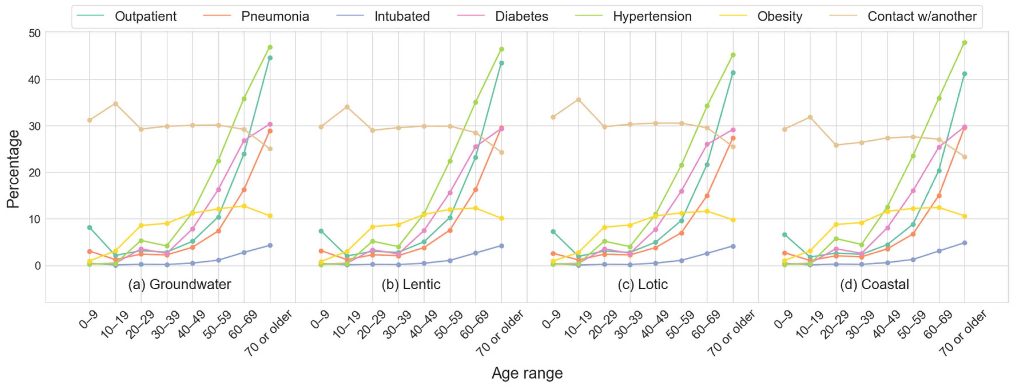
| Deaths | 173,209 (3.33% *) | 62,457 (3.22% *) | 173,844 (3.12% *) | 30,963 (2.94% *) |
| Survivors | 5,023,061 | 1,873,710 | 5,389,164 | 1,021,779 |
| Splits ** | 29 | 30 | 31 | 33 |
| (B) Description of cases for each dataset | ||||
| Outpatients | 4,803,252 | 1,793,986 | 5,164,581 | 986,164 |
| Hospitalized | 393,018 (7.56%) | 142,181 (7.34%) | 398,427 (7.16%) | 66,578 (6.32%) |
| Intubated | 37,691 (0.73%) | 13,512 (0.70%) | 39,462 (0.71%) | 8333 (0.79%) |
| Pneumonia | 271,642 (5.23%) | 100,555 (5.19%) | 281,343 (5.06%) | 49,223 (4.68%) |
| Hypertension | 587,770 (11.31%) | 214,885 (11.10%) | 613,269 (11.02%) | 120,638 (11.46%) |
| Obesity | 465,924 (8.97%) | 168,431 (8.70%) | 470,336 (8.45%) | 95,498 (9.07%) |
| Diabetes | 408,016 (7.85%) | 145,425 (7.51%) | 434,971 (7.82%) | 78,997 (7.50%) |
| Smoking | 237,501 (4.57%) | 93,173 (4.81%) | 262,268 (4.71%) | 38,129 (3.62%) |
| (C) Patients by medical units | ||||
| IMSS | 2,962,163 (57%) | 1,078,820 (55.72%) | 2,953,889 (53.10%) | 624,435 (59.32%) |
| ISSSTE | 168,299 (3.24%) | 57,734 (2.98%) | 162,208 (2.92%) | 36,640 (3.48%) |
| Military | 21,489 (0.41%) | 8686 (0.45%) | 23,616 (0.42%) | 8031 (0.76%) |
| Private | 268,790 (5.17%) | 192,214 (9.93%) | 301,219 (5.41%) | 71,945 (6.83%) |
| SSA | 1,620,706 (31.19%) | 514,482 (26.57%) | 1,960,516 (35.24%) | 280,491 (26.64%) |
| Others | 154,882 (2.98%) | 84,231 (4.35%) | 161,559 (2.90%) | 31,200 (2.96%) |
| Groundwater | Lentic | Lotic | Coastal | |
|---|---|---|---|---|
| (A) Mean position rank of features | ||||
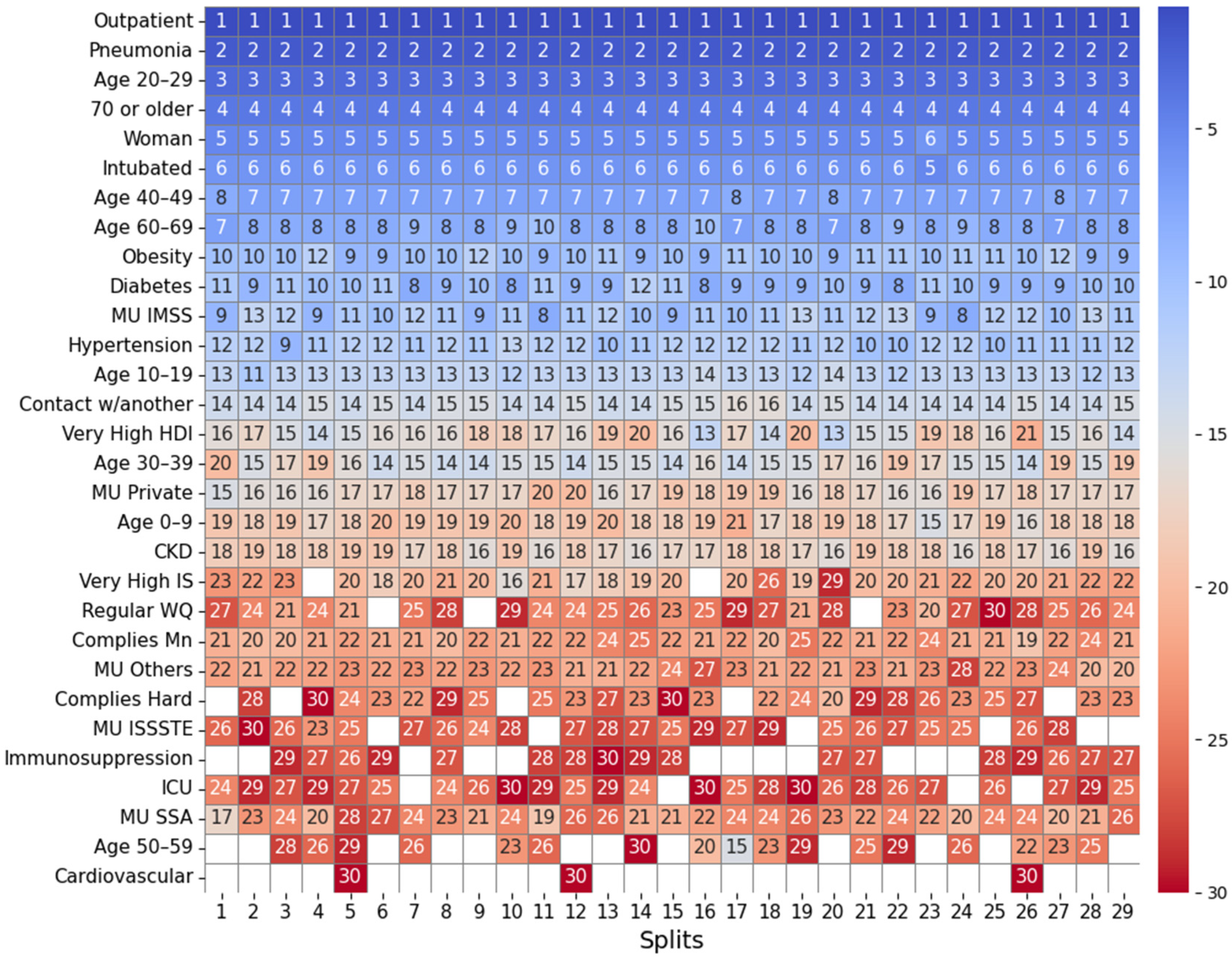
| Highest importance (1st–8th place) | Outpatient, pneumonia, age 20–29, 70 or older, woman, intubated, age 40–49, age 60–69 | Outpatient, pneumonia, age 20–29, 70 or older, woman, intubated, age 40–49, age 60–69 | Outpatient, pneumonia, age 20–29, 70 or older, woman, intubated, age 40–49, age 60–69 | Outpatient, pneumonia, age 20–29, intubated, 70 or older, woman, age 40–49, hypertension |
| High importance (9th–14th place) | Obesity, diabetes, MU IMSS, hypertension, age 10–19, contact w/another | Obesity, diabetes, hypertension, contact w/another, MU Private, age 10–19 | MU IMSS, diabetes, obesity, hypertension, age 10–19, very high HDI | age 60–69, diabetes, obesity, MU IMSS, age 10–19, MU Private |
| Mid-high importance (15th–19th place) | Very high HDI, age 30–39, MU private, age 0–9, CKD | MU IMSS, ODb, COD, good WQ, age 0–9 | Contact w/another, age 30–39, MU Private, CKD, age 0–9 | Contact w/another, age 0–9, CKD, MU SSA, age 30–39 |
| Mid importance (20th place and below) | MU SSA, Mn, MU Others, very high IS, regular water quality, ICU, hard, MU ISSSTE | MU Others, CKD, MU SSA, high HDI, ODs, age 30–39 | OD, ECOLI, MU SSA, FC, very high IS, MU Others, BOD5 | MU Others, very high IS, very high HDI, high IS, ICU, FC |
| (B) Frequency of water-related and socioeconomic features in the SHAP Top-30; the percentage of splits in which the variable ranked in the top 30 is shown in parentheses. | ||||
| Groundwater (total splits: 29) | Lentic (total splits: 30) | Lotic (total splits: 31) | Coastal (total splits: 33) | |
| Water-related features | Mn (ranked in the top-30 in 100% of splits), Hard (83%), F (48%), Fe (34%), TDS (14%), Cond (10%), As (3%), regular WQ (90%), good WQ (17%), poor water quality (14%) | ODb (ranked in the top-30 in 100% of splits), COD (100%), ODs (90%), ODm, (47%), ECOLI (23%), BOD5 (10%), good WQ (100%), poor WQ (50%), regular WQ (27%) | OD (ranked in the top-30 in 100% of splits), ECOLI (100%), FC (97%), BOD5 (84%), COD (45%), TD48 (22%), TSS (16%), TF15 (9%), regular WQ (39%), poor WQ (26%), good WQ (6%) | FC (ranked in the top-30 in 79% of splits), ODb (30%), FE (21%), ODs (3%), ODm (3%), regular WQ (64%), good WQ (52%) |
| Socioeconomic features | Very high HDI (100%), very high IS (93%), high IS (41%), high HDI (17%), medium HDI (7%) | High HDI (93%), high IS (83%), very high HDI (83%), very high IS (60%) | Very high HDI (100%), very high IS (93%), high IS (45%), medium IS (22%), high HDI (22%) | Very high IS (91%), very high HDI (91%), high IS (88%), medium IS (9%), high HS (3%) |
Disclaimer/Publisher’s Note: The statements, opinions and data contained in all publications are solely those of the individual author(s) and contributor(s) and not of MDPI and/or the editor(s). MDPI and/or the editor(s) disclaim responsibility for any injury to people or property resulting from any ideas, methods, instructions or products referred to in the content. |
© 2025 by the authors. Licensee MDPI, Basel, Switzerland. This article is an open access article distributed under the terms and conditions of the Creative Commons Attribution (CC BY) license (https://creativecommons.org/licenses/by/4.0/).
Share and Cite
Díaz-González, L.; Toribio-Colin, Y.S.; Pérez-Sansalvador, J.C.; Lakouari, N. Factors Associated with COVID-19 Mortality in Mexico: A Machine Learning Approach Using Clinical, Socioeconomic, and Environmental Data. Mach. Learn. Knowl. Extr. 2025, 7, 55. https://doi.org/10.3390/make7020055
Díaz-González L, Toribio-Colin YS, Pérez-Sansalvador JC, Lakouari N. Factors Associated with COVID-19 Mortality in Mexico: A Machine Learning Approach Using Clinical, Socioeconomic, and Environmental Data. Machine Learning and Knowledge Extraction. 2025; 7(2):55. https://doi.org/10.3390/make7020055
Chicago/Turabian StyleDíaz-González, Lorena, Yael Sharim Toribio-Colin, Julio César Pérez-Sansalvador, and Noureddine Lakouari. 2025. "Factors Associated with COVID-19 Mortality in Mexico: A Machine Learning Approach Using Clinical, Socioeconomic, and Environmental Data" Machine Learning and Knowledge Extraction 7, no. 2: 55. https://doi.org/10.3390/make7020055
APA StyleDíaz-González, L., Toribio-Colin, Y. S., Pérez-Sansalvador, J. C., & Lakouari, N. (2025). Factors Associated with COVID-19 Mortality in Mexico: A Machine Learning Approach Using Clinical, Socioeconomic, and Environmental Data. Machine Learning and Knowledge Extraction, 7(2), 55. https://doi.org/10.3390/make7020055


