Article

Factors Associated with COVID-19 Mortality in Mexico: A Machine Learning Approach Using Clinical, Socioeconomic, and Environmental Data

by
Lorena Díaz-González
1,*,
Yael Sharim Toribio-Colin
2,
Julio César Pérez-Sansalvador
3,4,* and
Noureddine Lakouari
3,4,*
1
Centro de Investigación en Ciencias, Universidad Autónoma del Estado de Morelos, Cuernavaca 62209, Morelos, Mexico
2
Licenciatura en Ciencias, Instituto de Investigación en Ciencias Básicas Aplicadas (IICBA), Universidad Autónoma del Estado de Morelos, Cuernavaca 62209, Morelos, Mexico
3
Department of Computer Science, Instituto Nacional de Astrofísica, Óptica y Electrónica, Luis Enrique Erro 1, Tonantzintla 72840, Puebla, Mexico
4
Secretaría de Ciencia, Humanidades, Tecnología e Innovación (SECIHTI), Insurgentes Sur 1582, Ciudad de Mexico 03940, Mexico
*
Authors to whom correspondence should be addressed.
Mach. Learn. Knowl. Extr. 2025, 7(2), 55; https://doi.org/10.3390/make7020055
Submission received: 26 April 2025 / Revised: 5 June 2025 / Accepted: 12 June 2025 / Published: 15 June 2025
(This article belongs to the Section Learning)

Abstract

COVID-19 mortality is a complex phenomenon influenced by multiple factors. This study aimed to identify factors associated with death in COVID-19 patients by considering clinical, demographic, environmental, and socioeconomic conditions, using machine learning models and a national dataset from Mexico covering all pandemic waves. We integrated data from the national COVID-19 dataset, municipal-level socioeconomic indicators, and water quality contaminants (physicochemical and microbiological). Patients were assigned to one of four datasets (groundwater, lentic, lotic, and coastal) based on their municipality of residence. We trained XGBoost models to predict patient death or survival on balanced subsets of each dataset. Hyperparameters were optimized using a grid search and cross-validation, and feature importance was analyzed using SHAP values, point-biserial correlation, and XGBoost metrics. The models achieved strong predictive performance (F1 score > 0.97). Key risk factors included older age (≥50 years), pneumonia, intubation, obesity, diabetes, hypertension, and chronic kidney disease, while outpatient status, younger age (<40 years), contact with a confirmed case, and care in private medical units were associated with survival. Female sex showed a protective trend. Higher socioeconomic levels appeared protective, whereas lower levels increased risk. Water quality contaminants (e.g., manganese, hardness, fluoride, dissolved oxygen, fecal coliforms) ranked among the top 30 features, suggesting an association between environmental factors and COVID-19 mortality.

1. Introduction

COVID-19 is a respiratory illness caused by the SARS-CoV-2 virus. On 30 January 2020, the World Health Organization (WHO) declared the COVID-19 epidemic a public health emergency of international concern, categorizing it as a pandemic on 11 March 2020, and subsequently announcing its end on 5 May 2023 [1,2]. The COVID-19 pandemic has profoundly impacted health systems globally, revealing vulnerabilities across varied socioeconomic contexts. In response to the crisis, numerous studies [3,4,5,6,7,8,9,10,11,12,13] have evaluated mortality factors associated with COVID-19, including clinical, comorbidities, socioeconomic, and environmental factors. These factors interact in complex ways and affect populations differently depending on their demographic and socioeconomic context [13]. However, many studies have focused on cohorts from the early pandemic stages within specific populations (e.g., smokers, hospitalized patients, or with specific comorbidities), leaving a gap in research that analyzes national databases from all COVID-19 waves, considering clinical, demographic, socioeconomic, healthcare access, and environmental factors.
Machine learning (ML) techniques have demonstrated significant effectiveness in identifying patterns within complex datasets and developing predictive models. The studies presented in this section applied ML methods to COVID-19 databases to identify factors associated with mortality risk, providing insight into clinical and socioeconomic influences. These studies employed diverse approaches:
(i)
Basic interpretable models: Decision trees and logistic regression are commonly used for their simplicity and interpretability [3].
(ii)
Ensemble models: Random forests and gradient boosting (e.g., CatBoost and eXtreme Gradient Boosting, XGBoost) are used for their superior accuracy and ability to capture complex interactions between variables [4,5,6,7,8,9,10,11,12,13].
(iii)
Distance-based models: Support vector machines (SVMs) and k-nearest neighbors (KNN) classify cases based on mathematical distances between data points, allowing pattern recognition in clinical datasets [8].
(iv)
Model explanation techniques: SHAP (Shapley additive explanations) has been used to quantify the feature contribution to COVID-19 mortality [4,5,7,9,11,12,13].
(v)
Feature selection techniques: BorutaSHAP [5,14] has been used to select the most relevant variables and improve model interpretability.
(vi)
Class-balancing techniques: SMOTE (synthetic minority oversampling technique) has addressed the imbalance in the dataset between the number of deaths and survivors by generating synthetic cases to better represent deaths [15].
The main factors associated with adverse outcomes are as follows: age; comorbidities such as diabetes, hypertension, chronic kidney disease (CKD), cardiovascular disease, and chronic obstructive pulmonary disease (COPD); inflammatory markers; socioeconomic factors such as HDI (Human Development Index); lifestyle factors such as smoking, dietary habits and body mass index (BMI); treatment; and level of care.
A detailed description of the main findings of each work follows:
  • Wollenstein-Betech et al. [3] studied a small first-wave dataset (91,000 cases) from Mexico using logistic regression without class balancing, identifying age, diabetes, renal failure, and immunosuppression as key risk factors for hospitalization and mortality. Their model achieved approximately 79% accuracy in mortality prediction. Rojas-García et al. [7] analyzed 11,564 COVID-19 cases without intubation and ICU from Morelos, Mexico, using XGBoost and SHAP without class balancing, reporting an AUC of 0.85 and highlighting diabetes and chronic kidney disease as major risk factors. Carvantes et al. [11] analyzed a larger dataset (5,566,732 cases) of confirmed COVID-19 patients in Mexico across four epidemiologic waves (February 2020–April 2022), developing predictive models with XGBoost and SHAP. Their best models achieved AUC values between 0.83 and 0.86, identifying pneumonia and advanced age as the highest risk factors and identifying medical unit type (IMSS vs. SSA) as a significant risk or protective factor. Other contributing risk factors included intubation (notably in the first wave), diabetes, obesity, hypertension, and residence in low-HDI municipalities.
  • Khadem et al. [4] studied 505 COVID-19 patients with and without diabetes mellitus (DM) in a UK hospital during the first wave, identifying neutrophil-lymphocyte ratio (NLR), and sodium as mortality risk factors in DM patients, while albumin, estimated glomerular filtration rate (eGFR), and age were identified as risk factors non-DM patients. They used random forests without class balancing, SHAP for interpretation, and K-means for risk stratification.
  • Barría-Sandoval et al. [5] analyzed 57,623 records on chronic diseases and COVID-19 mortality from Chile, identifying age and place of death as primary predictors using XGBoost, BorutaSHAP, and SHAP without class balancing.
  • Datta et al. [6] studied 5371 hospitalized COVID-19 patients in South Florida, highlighting age, diabetes, hypertension, and chronic kidney disease as risk factors using Random Forest and SMOTE for class balancing.
  • Sharifi-Kia et al. [9] examined 678 COVID-19 patients with a smoking history across six Iranian hospitals, identifying age, smoking, oxygen saturation, body mass index (BMI), and blood pressure as risk factors using SMOTE, XGBoost, and SHAP.
  • Casillas et al. [10] analyzed 684 ICU COVID-19 patients in two Spanish hospitals across six pandemic waves, identifying age, BMI, ferritin, lactate dehydrogenase, C-reactive protein levels, invasive ventilation, and clotting times as key predictors using XGBoost.
  • Zhou et al. [12] analyzed global data from 156 countries with XGBoost and SHAP, identifying vaccination, population aging, and healthcare coverage as global risk factors and highlighting distinct geographical patterns in mortality rates.
  • Chu et al. [13] reported correlations between COVID-19 hospitalization rates, atmospheric NO2 concentration, and workforce education at the municipal level in Germany, suggesting that socioeconomic and air quality factors play a role in pandemic mortality patterns.
These studies e.g., [4,5,7,8,9,11,12] have demonstrated the utility of SHAP values in identifying important risk factors for COVID-19 mortality. For instance, Khadem et al. identified key biomarkers in diabetic and non-diabetic COVID-19 patients, while Rojas-García et al. identified diabetes and chronic kidney disease as risk factors in a specific subgroup of COVID-19 patients (non-intubated and non-ICU).
These previous studies underscore the need for a comprehensive analysis including clinical, comorbidities, socioeconomic, and environmental factors to improve risk prediction in future epidemiological crises, reduce mortality in vulnerable populations, and optimize public health strategies, especially in countries such as Mexico, which experienced high COVID-19 lethality. This study addresses these gaps by analyzing a comprehensive national database from Mexico, covering all waves of COVID-19, including clinical, demographic, socioeconomic, healthcare access, and water quality factors. These data were sourced from the National Epidemiologic Surveillance System [16], including only laboratory-confirmed or epidemiologically associated COVID-19 cases. This study covers the period from 19 February 2020, to 28 February 2023, with a total of 9,963,368 survivors and 307,204 deaths.

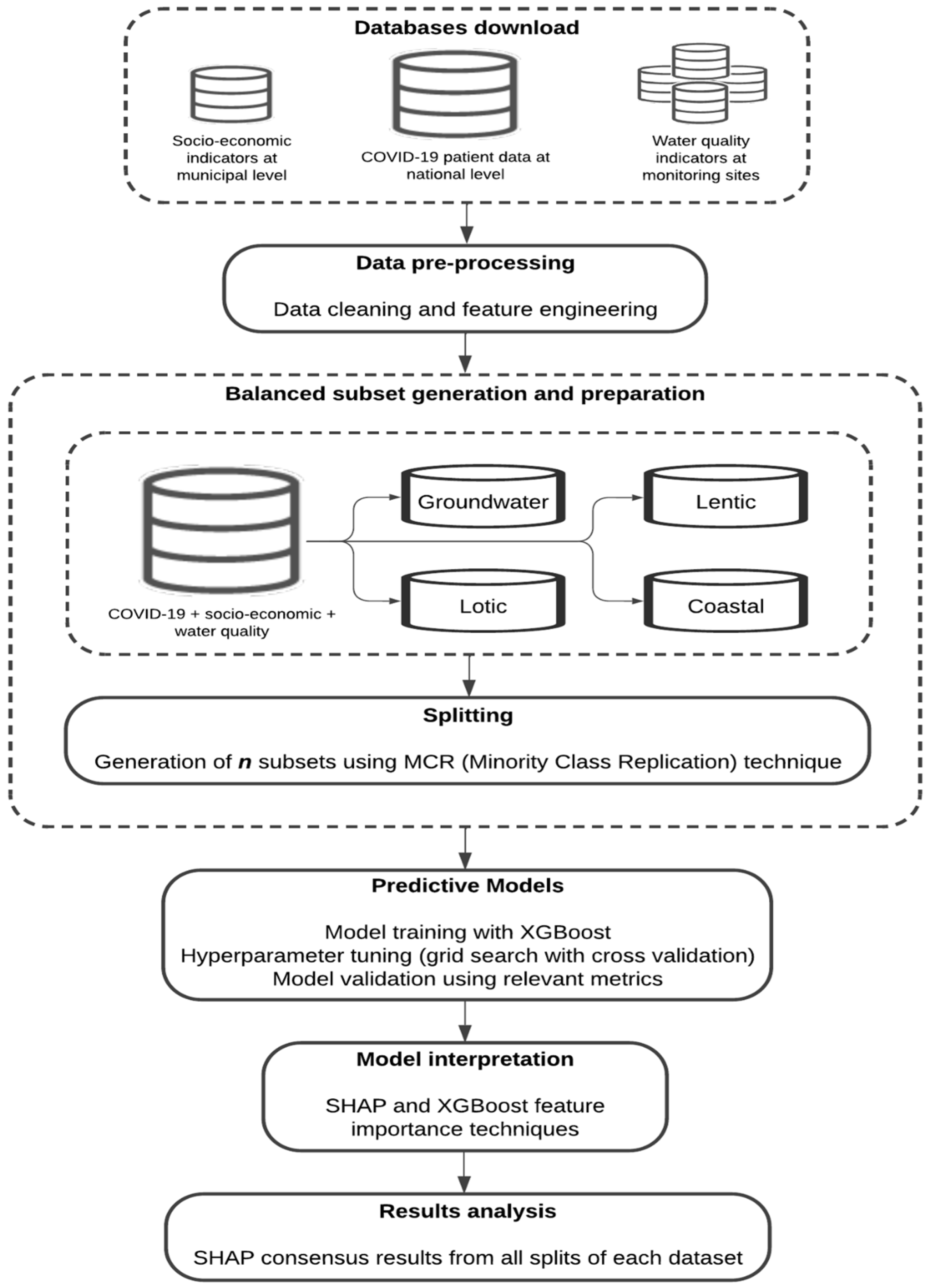
2. Methods and Materials

Figure 1 illustrates the general methodology applied in this study.

2.1. Databases

This section details the preprocessing and analysis steps applied to the datasets, including database download, data cleaning, feature engineering, dataset segmentation, balanced subset generation, and data preparation for machine learning tasks.

2.1.1. Database Download

Three data sources were used in this research:
(a)
COVID-19 database. This database, containing all confirmed, suspected, negative, and death cases, was downloaded from the Mexican government website [16].
(b)
Socioeconomic indicators. Municipal-level Human Development Index (HDI), and health (HS) and income (IS) subindexes, reported by the United Nations Development Programme [17] and collected by the National Council for Social Development Policy Evaluation [18], were assigned to each patient according to their municipality of residence. The most recent socioeconomic data from 2020 were used, as these are reported every 5 years. Four levels were defined for each variable, ranging from 0 to 1: very high (0.800–1.000), high (0.700–0.799), medium (0.551–0.699), and low (0.000–0.550). These indices were added as additional patient characteristics to analyze the impact of socioeconomic vulnerability on COVID-19 mortality, considering that impoverished populations often face greater health risks than those with better economic opportunities [19].
(c)
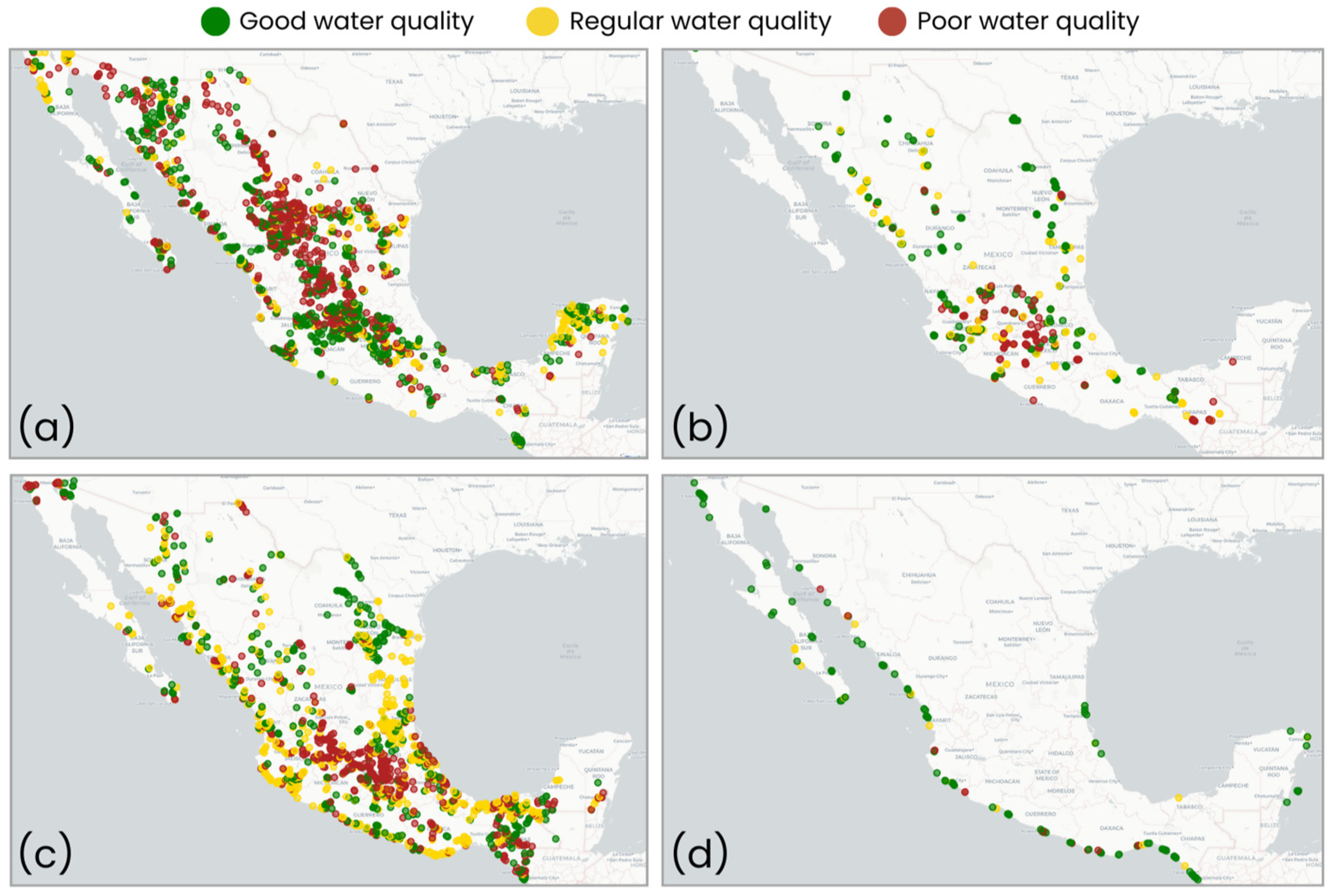
Water quality parameters. The National Water Commission database [20] reports various contaminants and classifies water as good, regular, or poor at monitoring sites for four water body types: groundwater, lentic, lotic, and coastal (Table A1; [21]). The most recent data from 2018 to 2022 were used. Water quality classification was assigned as follows: (i) Groundwater: Regular quality indicates non-compliance with permitted levels for any of the following contaminants: alkalinity (Alk), conductivity (Cond), hardness (Hard), total dissolved solids (TDS), iron (Fe), or manganese (Mn). Poor quality indicates non-compliance for fluorides (F), fecal coliforms (FC), nitrate-nitrogen, or heavy metals such as arsenic (As), cadmium (Cd), chromium (Cr), mercury (Hg), and lead (Pb). (ii) Surface (lentic, lotic, and coastal) water: Regular quality indicates non-compliance for total suspended solids (TSS), FC, Escherichia coli (ECOLI), or percent oxygen saturation (surface ODs, medium ODm, and background ODb levels). Poor quality indicates non-compliance for any of the following higher risk parameters: 5-day biochemical oxygen demand (BOD5), chemical oxygen demand (COD), fecal enterococci (FE), or toxicity (Daphnia Magna 48 h, Vibrio Fischeri 15 min). Finally, good water quality is defined by compliance with all physicochemical and microbiological contaminants (Table A1).
Each COVID-19 patient was assigned a global water quality (WQ) classification (good, regular, or poor quality) and a set of individual water quality contaminants (e.g., Alk, Cond, Hard, TDS, Fe, Mn, etc.) from the monitoring site in their municipality of residence. The global classification reflects overall water quality, while individual contaminants reflect compliance status for each specific pollutant according to environmental standards (Table A1).

2.1.2. Data Cleaning and Imputation

The following data cleaning and imputation steps were applied to the integrated databases:
(i)
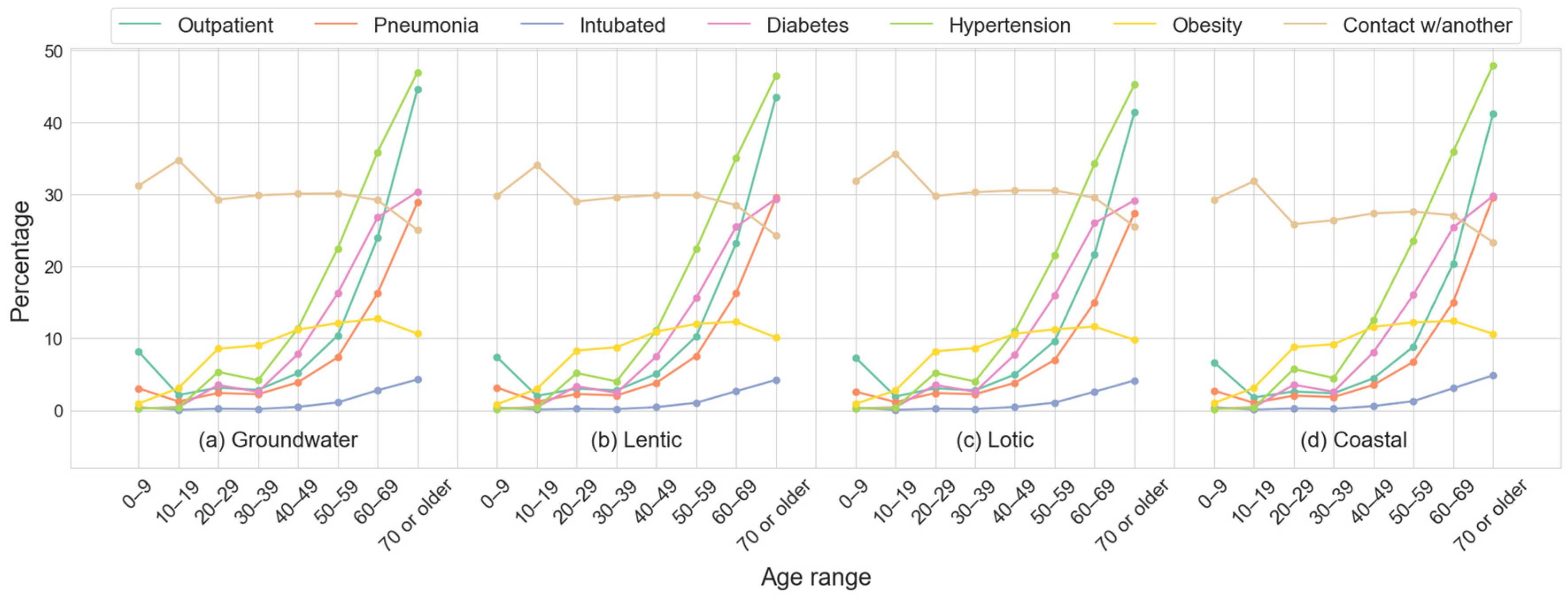
COVID-19 data cleaning: Only confirmed positive cases between 19 February 2020, and 28 February 2023, were considered, totaling 13,494,572 cases, of which 990,542 were hospitalized and 436,138 deceased. The selected variables included: (i) comorbidities: diabetes, hypertension, obesity, cardiovascular disease, chronic kidney disease (CKD), smoking, chronic obstructive pulmonary disease (COPD), asthma, and immunosuppression); (ii) patient characteristics: sex, age, hospitalized or outpatient status, pneumonia, intubation, and intensive care unit (ICU) admission; (iii) medical units: IMSS (Mexican Social Security Institute), ISSSTE (Institute of Social Security and Services for State Workers), SSA (Secretariat of Health), military, private, and other; and (iv) outcome variable: patient survival status (alive or dead). Cases with missing values in any of the selected variables were excluded from the analysis.
(ii)
Socioeconomic data imputation: For 570 municipalities in Oaxaca, socioeconomic indicators (HDI, HS, and IS) are reported by region [18]. Therefore, the state average was assigned to these municipalities.
(iii)
Water quality data imputation: Due to missing values across multiple municipalities, a state-label imputation was applied separately for each water body type. For states with >30% missing data, values were imputed based on geographic proximity by copying data from neighboring municipalities. For states with ≤30% missing data, the proportion of water quality ratings was calculated at the state level, and missing values were assigned randomly while maintaining the original distribution.

2.1.3. Feature Engineering

All variables were converted to binary format (1 = presence, 0 = absence). Age was categorized into eight groups: 0–9, 10–19, 20–29, 30–39, 40–49, 50–59, 60–69, and 70+ years old. Binary variables were also generated to encode the predefined socioeconomic and water quality categories, as previously described.

2.1.4. Integration of COVID-19 and Water Quality Databases

The COVID-19 database was merged with water quality data by linking patients to their municipality of residence. The integrated dataset was then divided into four subsets based on water body type: groundwater, lentic, lotic, and coastal. Patients from municipalities with multiple water body types were included in each relevant dataset.
Special consideration was required when assigning the water quality data, as there are multiple measurements for a single municipality. All available measurements were considered and randomly assigned to patients from the same locality, according to the following rule: Let m be the number of patient records in the COVID-19 database for a given municipality and n be the number of water quality records for the same municipality. If m > n, the water quality records (n) were repeated k times to cover most patient records, and the remaining r patient records of m were randomly sampled from n without replacement, such that m = kn + r; otherwise, a random sample without replacement of size m was taken from n water quality records. This approach preserves variability in water quality measurements while appropriately linking the data to COVID-19 records for subsequent analysis.
The complete datasets comprised a total of 59, 57, 53, and 53 variables for groundwater, lentic, lotic, and coastal datasets, respectively. These included 30 variables related to COVID-19 clinical and demographic data, 12 to socioeconomic conditions, and 11–17 to water quality contaminants, depending on the water body type.

2.1.5. Demographic and Clinical Features Description Across Datasets

The analyzed cohorts, shown geographically in Figure 2, consist of groundwater, lentic, lotic, and coastal datasets, with respective death counts of 173,209; 62,457; 173,844; and 30,963. Survivor counts are 5,023,061; 1,873,710; 5,389,164; and 1,021,779, resulting in lethality rates of 3.3%, 3.2%, 3.1%, and 2.9%, respectively (see Table 1).
Each dataset contains a similar distribution of clinical and demographic characteristics, including outpatient, hospitalized, intubated, and pneumonia cases, as well as comorbidities such as hypertension, obesity, diabetes, and smoking. Key patterns in Table 1 include: (a) outpatients represent ~93% of cases in all datasets; (b) hospitalized cases account for ~7% of total cases; (c) intubated patients represent <1%, with minimal variation across datasets; (d) pneumonia cases range from 4.7% in the coastal dataset to 5.2% in the groundwater dataset; (e) hypertension affects ~11% of patients across all cohorts; (f) obesity rates range from 8.5% to 9.1%, highest in the coastal dataset; (g) diabetes prevalence is ~7.5% to 7.8%; and (h) smoking is the least common, ranging from 3.6% in the coastal dataset to 4.8% in the lentic dataset.
Table 2 also shows the distribution of patients among medical institutions. IMSS attended the most cases (>50% in all datasets, peaking at 59.32% in the coastal dataset). SSA was the second most significant provider (26.57% in the lentic dataset to 35.24% in the lotic dataset). Private institutions varied, most prominent in the lentic dataset (9.93%). ISSSTE, the military, and others contributed smaller percentages. ISSSTE had a slightly higher presence in the coastal dataset (3.48%).
Figure 3 illustrates consistent demographic and clinical characteristics across all datasets. This statistical analysis of age groups (0–9, 10–19, 20–29, 30–39, 40–49, 50–59, 60–69, and 70+ years old) provides essential context for understanding the behavior in the models and the relative importance of mortality risk factors. Notably, comorbidity prevalence and COVID-19 complications increase significantly from age 40. This pattern underscores the increased susceptibility of older populations to severe outcomes associated with COVID-19.

2.1.6. Balanced Subsets Generation and Preparation

The datasets analyzed exhibit varying degrees of class imbalance between survivors and deaths, with lethality rates ranging from 2.9% to 3.3%. To address this imbalance, multiple subsets (splits) were generated for each dataset, maintaining a 50%-50% ratio of deaths to survivors, using minority class replication. All death records were reused across splits, while an equivalent number of survivors were randomly selected. Any remaining records (0.8–1.3% of the total dataset) were excluded for consistency. We generated 29, 30, 31, and 33 balanced splits for the groundwater, lentic, lotic, and coastal datasets, respectively. A separate model was trained for each split, resulting in a total of 123 trained models.

2.2. XGBoost Models Training

Decision tree-based algorithms are highly effective for classification tasks, and boosting techniques enhance their predictive performance. One of the most powerful and widely used boosting algorithms is XGBoost (eXtreme Gradient Boosting), known for its efficiency, scalability, and high performance. This section provides an overview of XGBoost’s key concepts, including decision tree construction, boosting mechanics, gradient descent optimization, and feature importance evaluation, which are essential to understanding its functionality.
XGBoost uses decision trees as base learners [22] in the boosting process. Each tree is built using a recursive partitioning algorithm that splits data into subsets based on feature values. The goal is to minimize prediction error by selecting the best feature and threshold at each node. This process creates a tree where each branch corresponds to a decision rule, improving predictions by isolating meaningful patterns.
The algorithm follows a greedy approach, evaluating all possible splits at each step and selecting the one that minimizes loss. Split selection is guided by a criterion, such as information gain, which measures homogeneity using entropy [23].
The model is optimized using an objective function that combines two components: (i) the loss function (logarithmic loss for classification), which measures prediction error; and (ii) regularization terms, L1 (Lasso) and L2 (Ridge), which prevent overfitting by penalizing model complexity.
Optimization is performed using gradient descent, adjusting parameters iteratively to minimize loss. Unlike traditional gradient descent, XGBoost incorporates this process into the boosting framework, progressively improving performance over iterations.
Boosting is an ensemble technique that combines weak models to create a strong one. In XGBoost, trees are added sequentially, with each new tree correcting errors from the previous one by assigning higher weights to misclassified instances. Each new tree predicts residual errors of the current model based on the loss function gradient concerning the current predictions, thus progressively refining the model.
XGBoost also provides insights into feature importance through three embedded metrics [24]: (i) gain (loss reduction achieved by splits on a feature), (ii) weight (frequency of use of a feature in splits), and (iii) cover (number of records affected by a feature in splits). These metrics enhance model interpretability by revealing decision-making processes and variable importance.

Hyperparameter Tuning and Cross-Validation

The XGBoost framework (version 2.1.1) for Python (version 3.12.2) was used to build the predictor models. Each balanced subset was split into 80% training and 20% testing.
Hyperparameter tuning was conducted via a grid search [25] with five-fold stratified cross-validation. The training data was divided into five folds, with four used for training and one for validation in each iteration. This process was repeated five times, ensuring that every observation was used for both training and validation. The best hyperparameters were selected based on average accuracy across folds.
For each subset, seven hyperparameters of XGBoost [26] were tuned in four sequential steps due to computational cost: 1. max_depth and min_child_weight; 2. gamma; 3. subsample and colsample_bytree; and 4. reg_lambda and n_estimators. These hyperparameters, their default values, and the evaluated ranges are as follows:
  • max_depth: Maximum tree depth (default = 6; range: [0, ∞]; values evaluated: [3–10]).
  • min_child_weight: Minimum sum of instance weights in a child node (default = 1, range = [0, ∞]; values: [3–6]).
  • gamma: Minimum loss reduction to create a partition (default = 0, range = [0, ∞]; values: [0–0.5 in increments of 0.1]).
  • subsample: Fraction of training samples per tree (default = 1, range = [0, 1]; values: [0.1–1.0 in increments of 0.1]).
  • colsample_bytree: Fraction of features used per tree (default = 1, range = [0, 1]; values [0.2–1.0 in increments of 0.1]).
  • reg_lambda: L2 regularization on weights (default = 1, range = [0, ∞]; values: [0.3–1.0 in increments of 0.1]).
  • n_estimators: Number of boosting iterations (default = 100, range = [1, ∞]; values: [50, 100, 150]).
After selecting the optimal hyperparameters, each model was retrained using the full training set (80%), and the final performance was evaluated on the test set (20%).

2.3. XGBoost Model Evaluation

Classification model performance was evaluated using metrics derived from the confusion matrix [27]: true positives (TP), false positives (FP), true negatives (TN), and false negatives (FN). Metric averages were calculated across all splits to summarize the performance of each dataset. Performance metrics were as follows:
Accuracy (Equation (1)): The ratio of correctly predicted instances (TP and TN) to the total number of cases, which is useful but can be misleading for imbalanced datasets.
Precision (Equation (2)): The proportion of true positives among all positive predictions, which is crucial when false positives are costly.
Recall (Sensitivity; Equation (3)): The proportion of actual positives correctly identified, which is critical when reducing false negatives is a priority.
F1 Score (Equation (4)): The harmonic mean of precision and recall, which is useful for unbalanced datasets.
Matthews Correlation Coefficient (MCC; Equation (5)): Accounts for all components of the confusion matrix, which is effective for imbalanced datasets.
A c c u r a c y = T P + T N T P + F P + T N + F N
P r e c i s i o n = T P T P + F P
R e c a l l = T P T P + F N
F 1   S c o r e = 2 · P r e c i s i o n · R e c a l l P r e c i s i o n + R e c a l l
M C C = T P · T N F P · F N T P + F P T P + F N T N + F P T N + F N

2.4. XGBoost Model Interpretation with SHAP

SHAP [28,29] is a widely used method for interpreting machine learning models based on cooperative game theory. It assigns a contribution score to each feature, quantifying their impact on the model’s predictions. These contributions are computed by considering all possible feature combinations, ensuring a fair distribution of importance.
The Shapley value for a feature is the average of its marginal contributions across all feature combinations. This additive property allows both local interpretability (individual prediction explanations) and global interpretability (overall feature influence). SHAP effectively handles complex and nonlinear models, such as XGBoost, and captures feature interactions that traditional methods might miss. It also enables intuitive visualization, enhancing interpretability, transparency, and trust. In predicting COVID-19 mortality, a high positive SHAP value indicates an increased risk of death. Shapley values were computed using an XGBoost binary model with the SHAP framework (version 0.46.0) in Python.

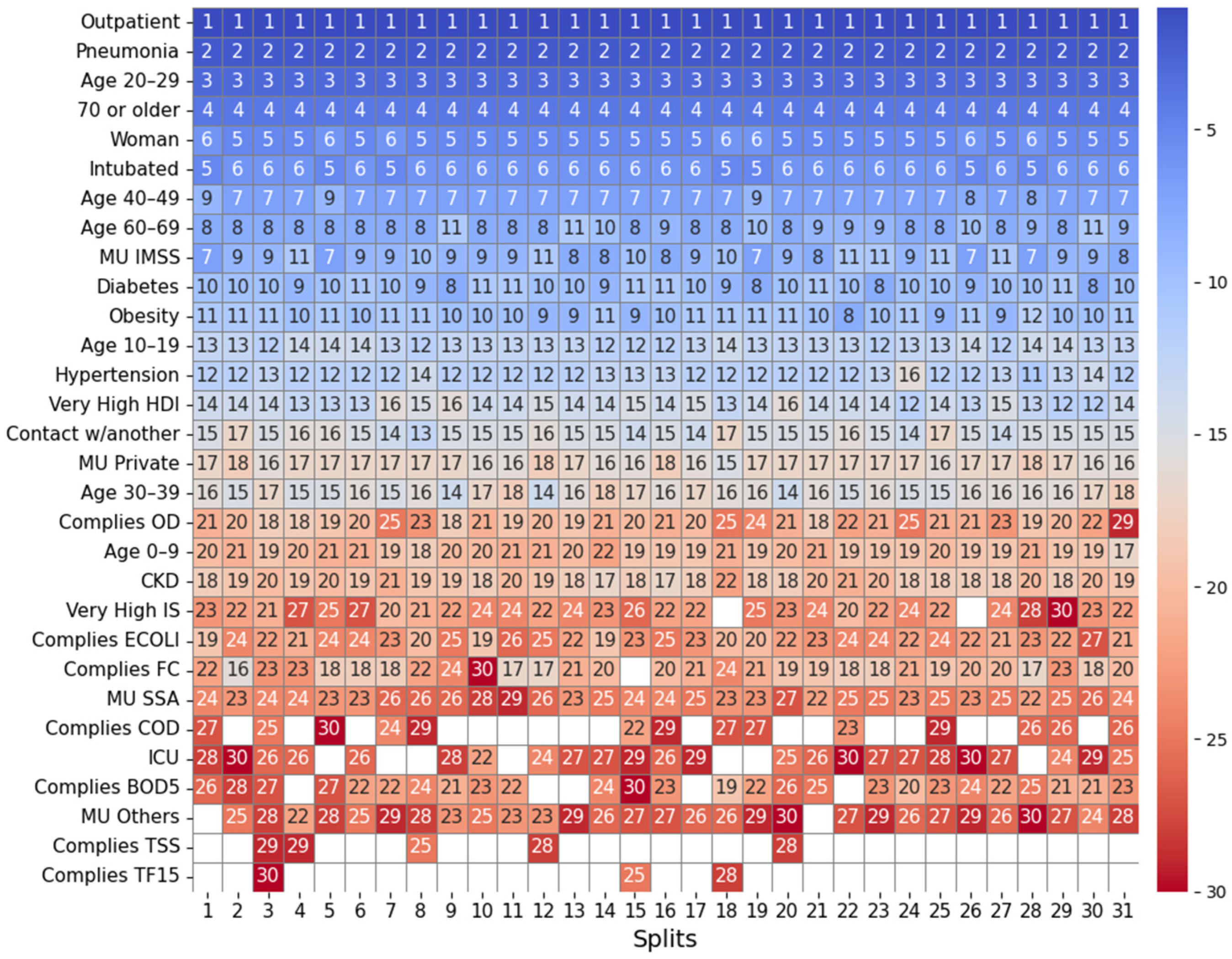
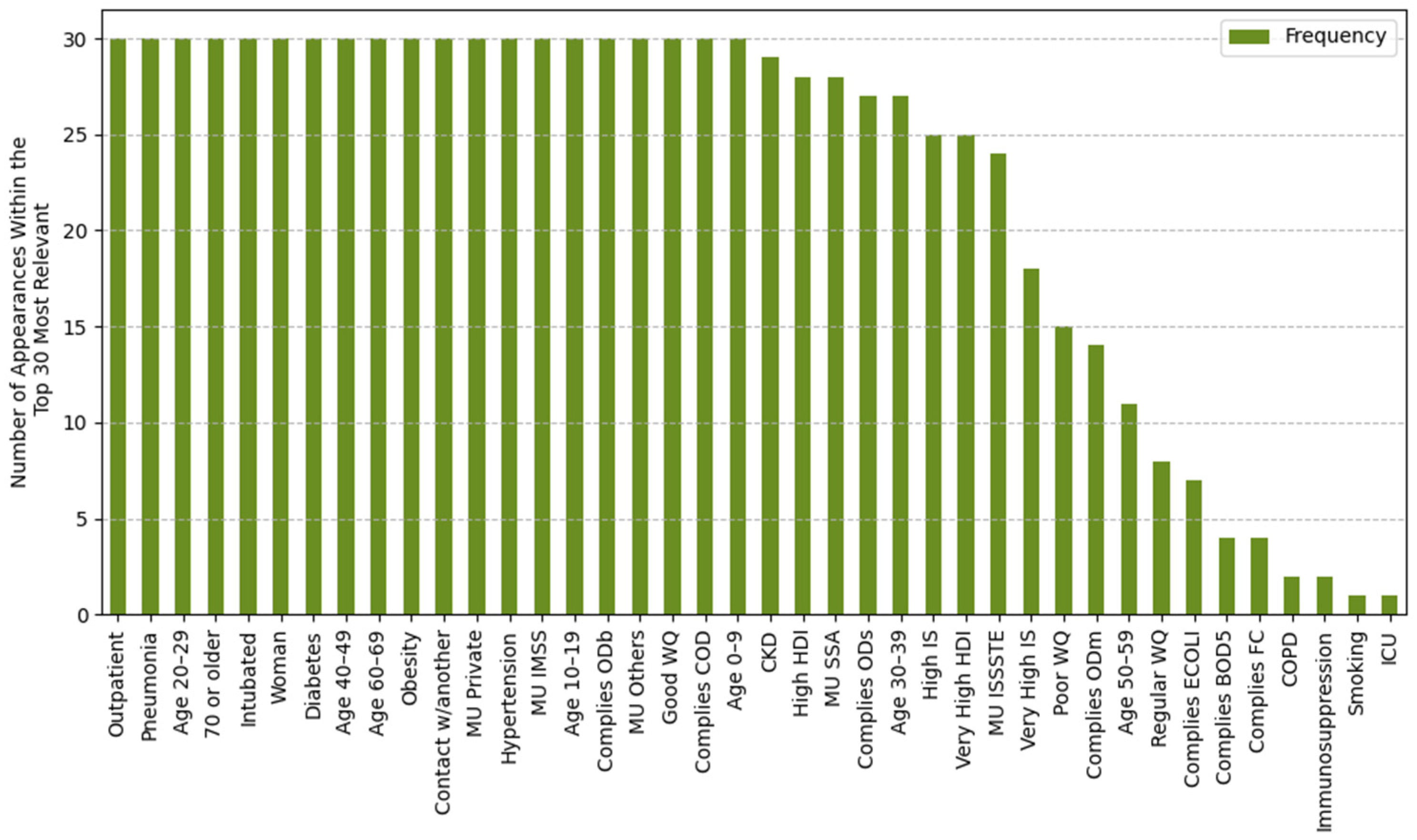
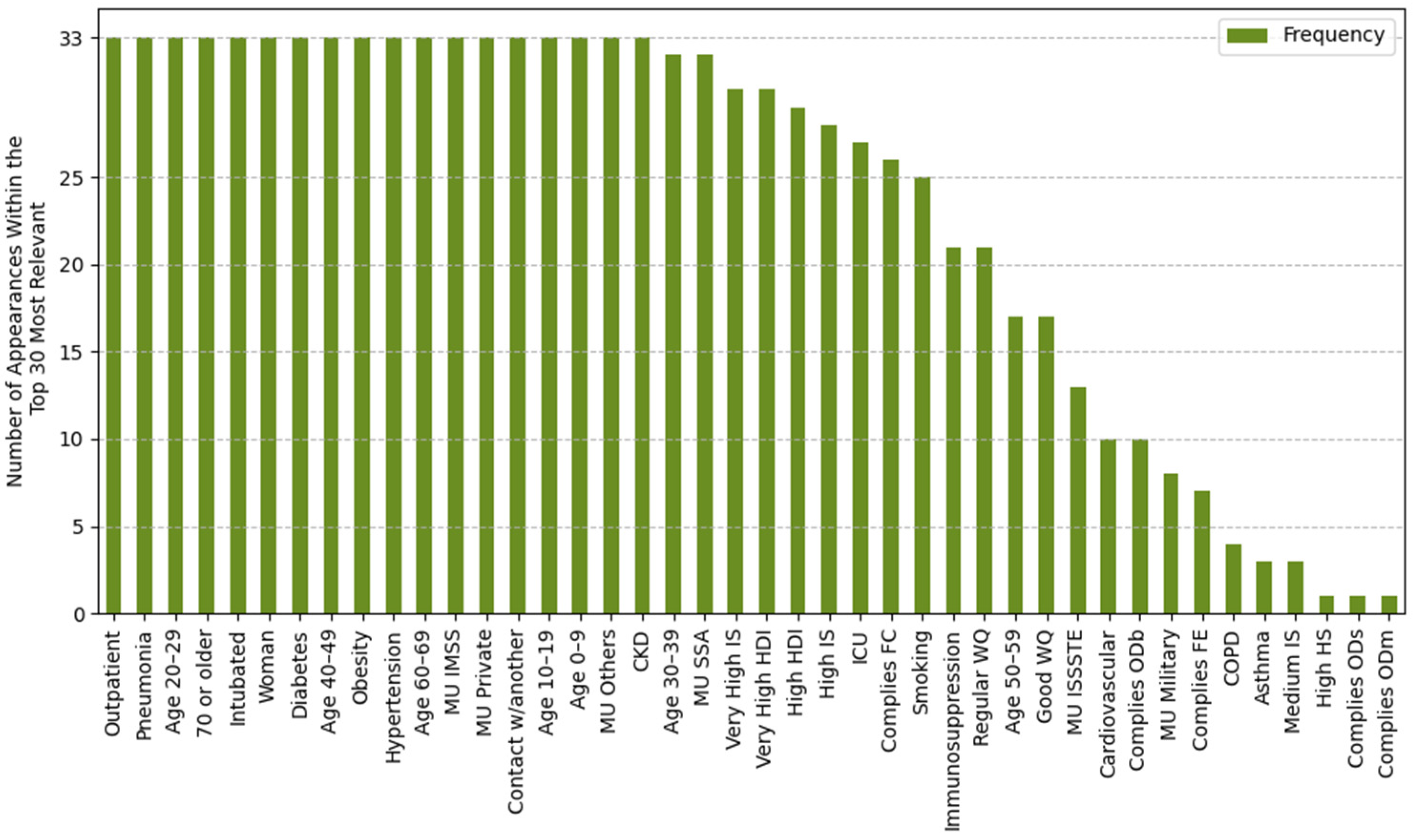
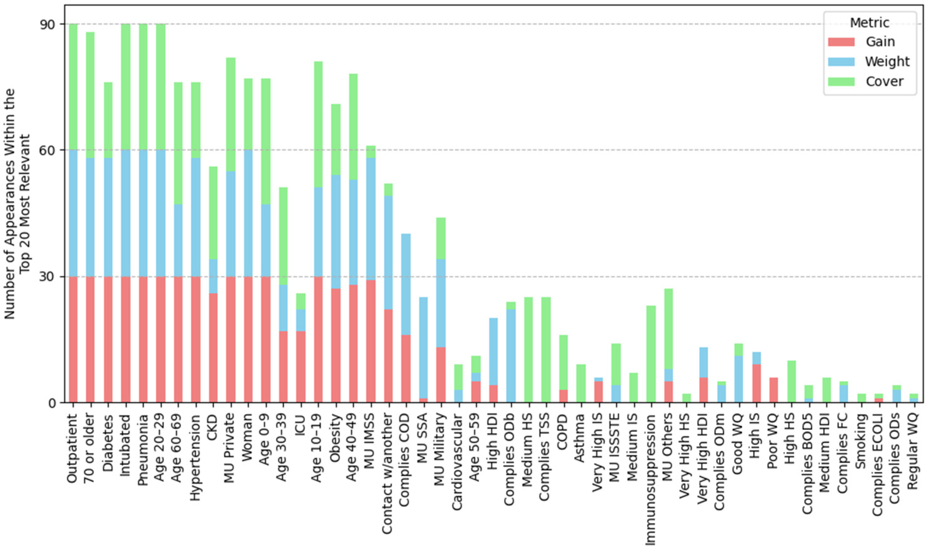
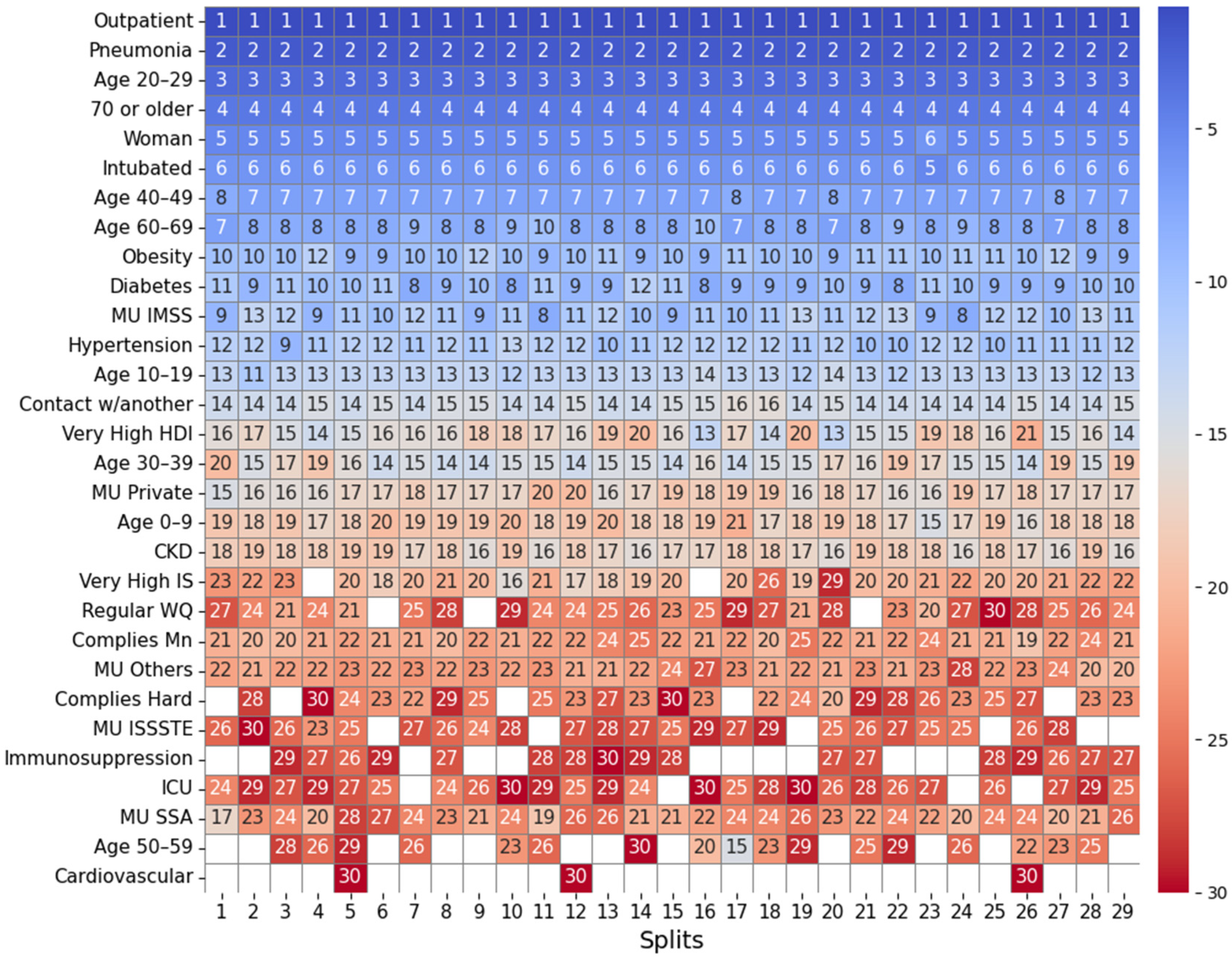
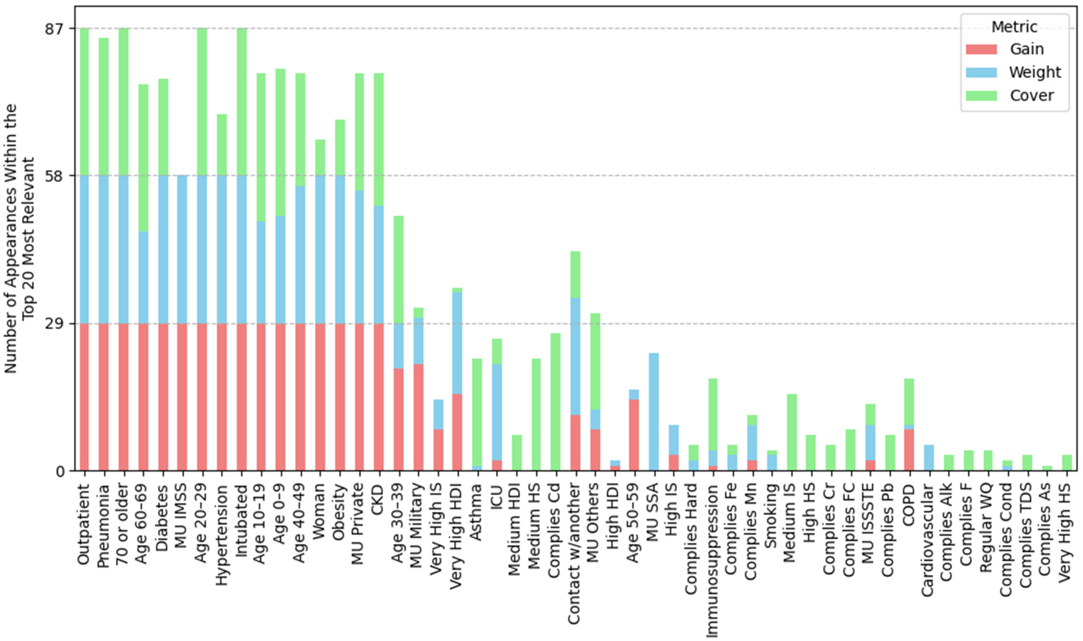
2.4.1. Feature Importance Based on Top 30 SHAP Rankings Across All Splits

SHAP values were used to identify the top 30 most important features in each model. A frequency count was used to determine how often each feature appeared within this threshold across all models for each dataset. This method highlights consistently relevant features and differentiates them from those excluded in some models because each model represents a different data partition.

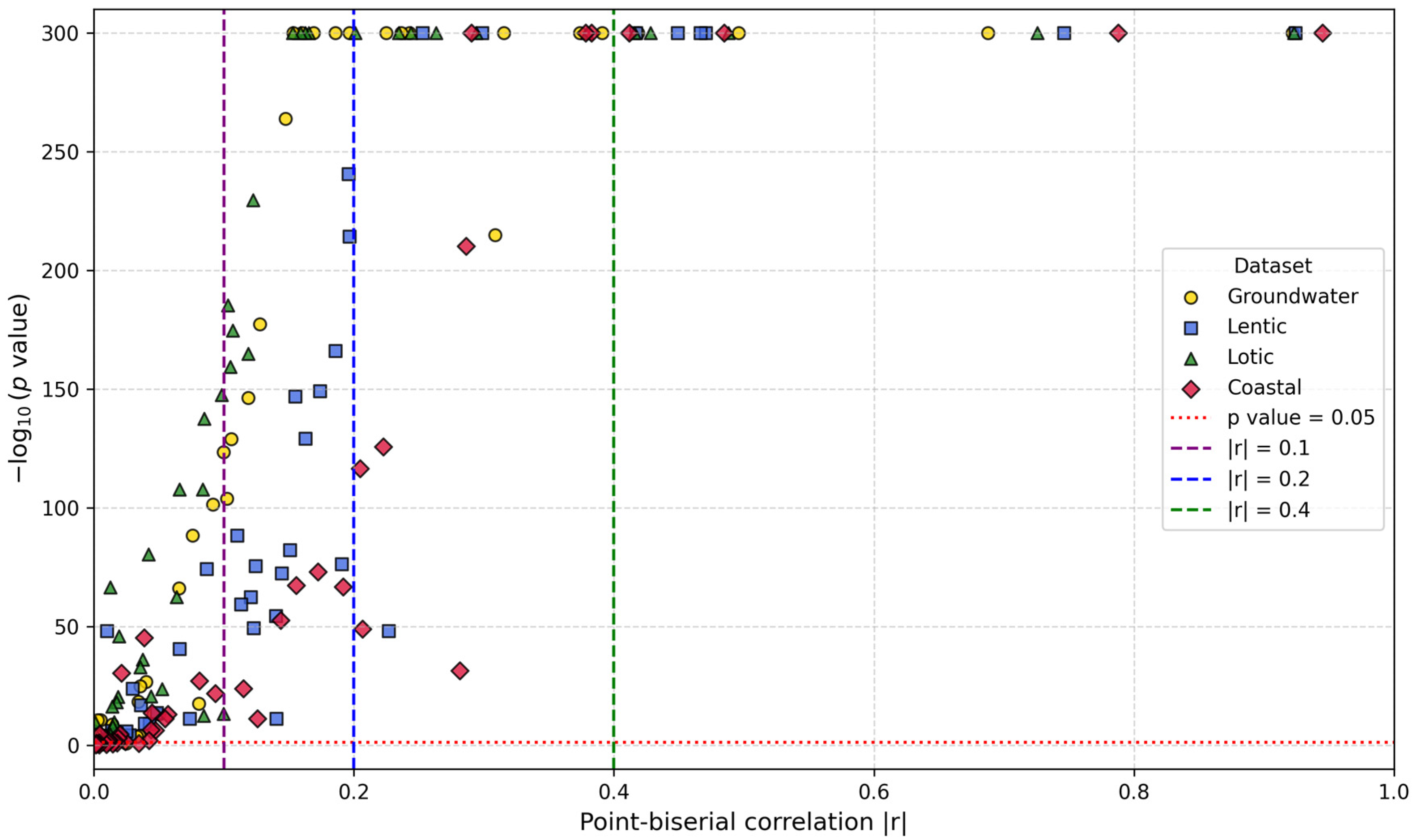
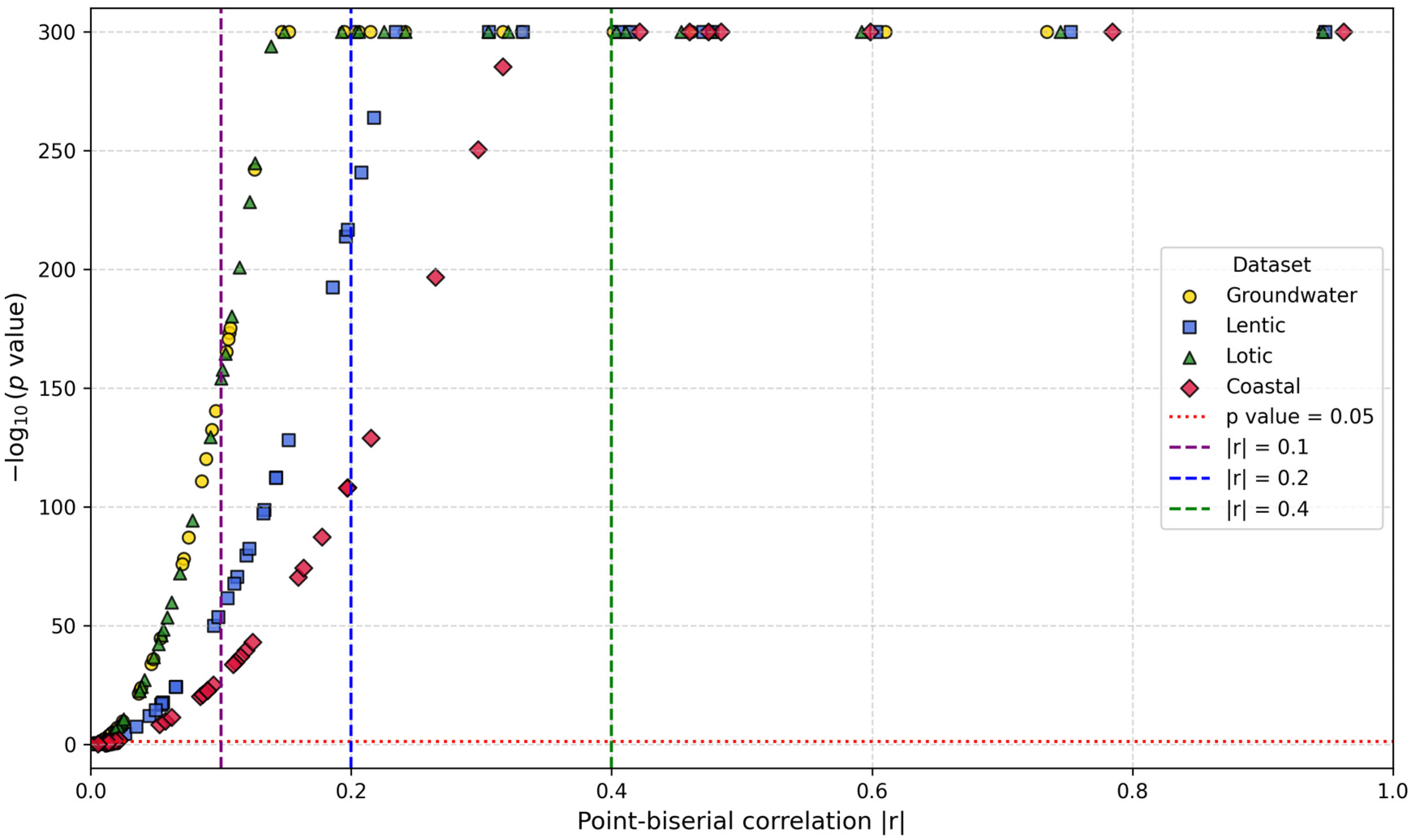
2.4.2. Feature Importance Based on Point-Biserial Correlation Across All Splits

Point-biserial correlation ([30], Equation (6)) measures the relationship between a continuous variable (SHAP values) and a binary variable (patient status: 0 = survivor, 1 = deceased). Values range from −1 to +1.
c o r r e l a t i o n = A B s n A · n B n 2
where A and B are the means of the continuous variable for the two groups, s is the standard deviation of the continuous variable, nA and nB are the group sizes, and n is the total sample size.
This correlation summarized the SHAP values from all models in each dataset. Two strategies were applied:
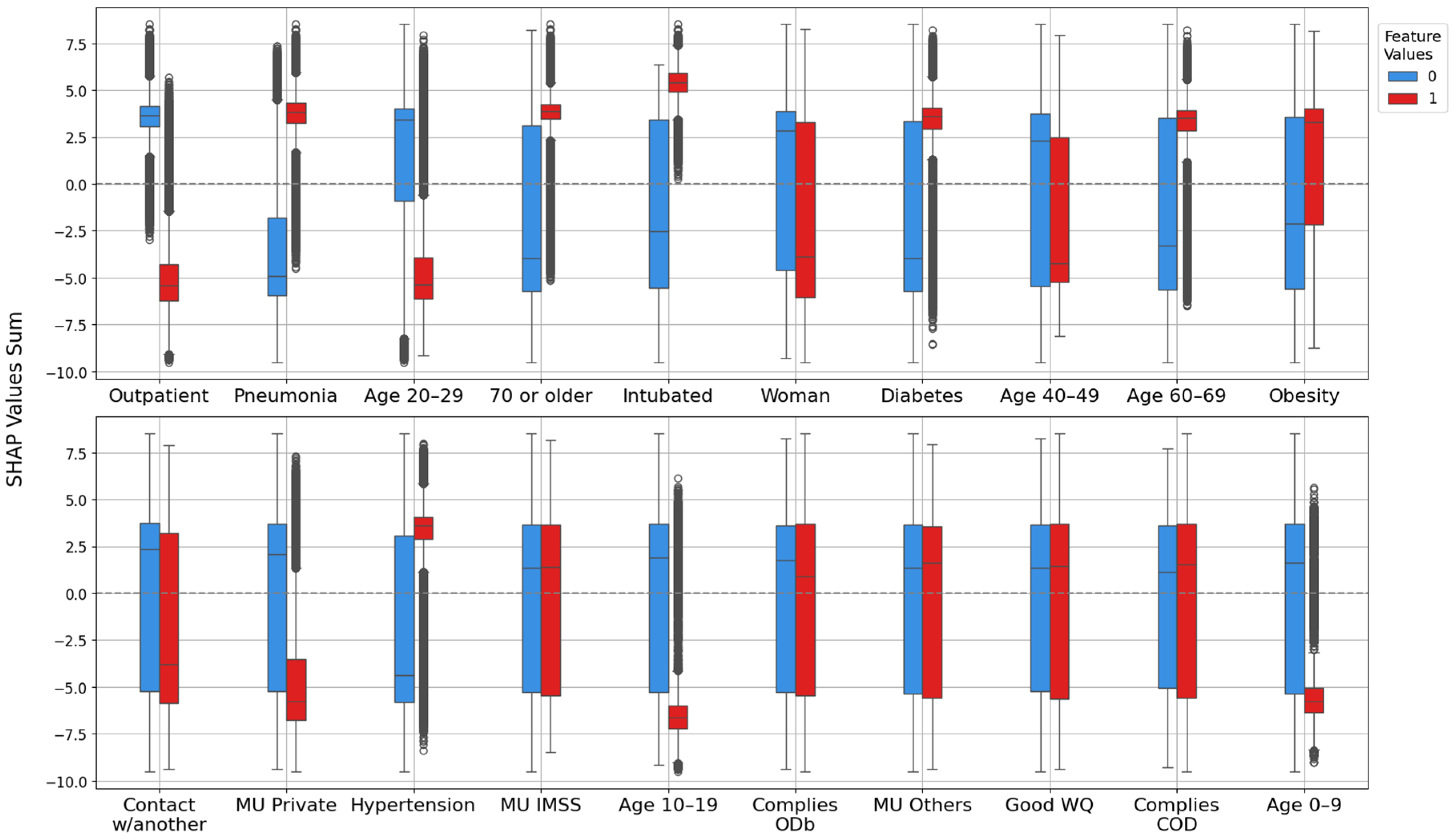
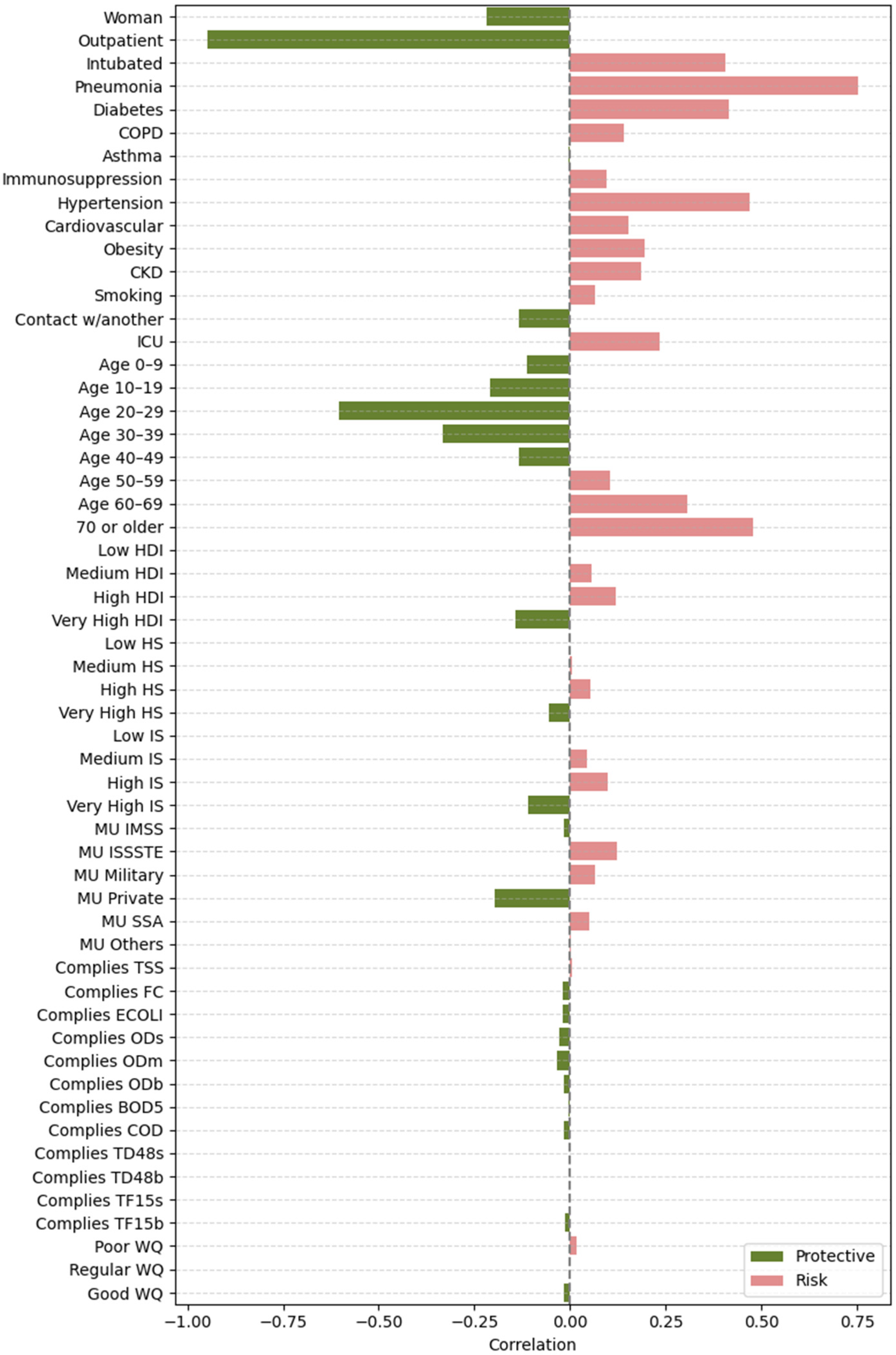
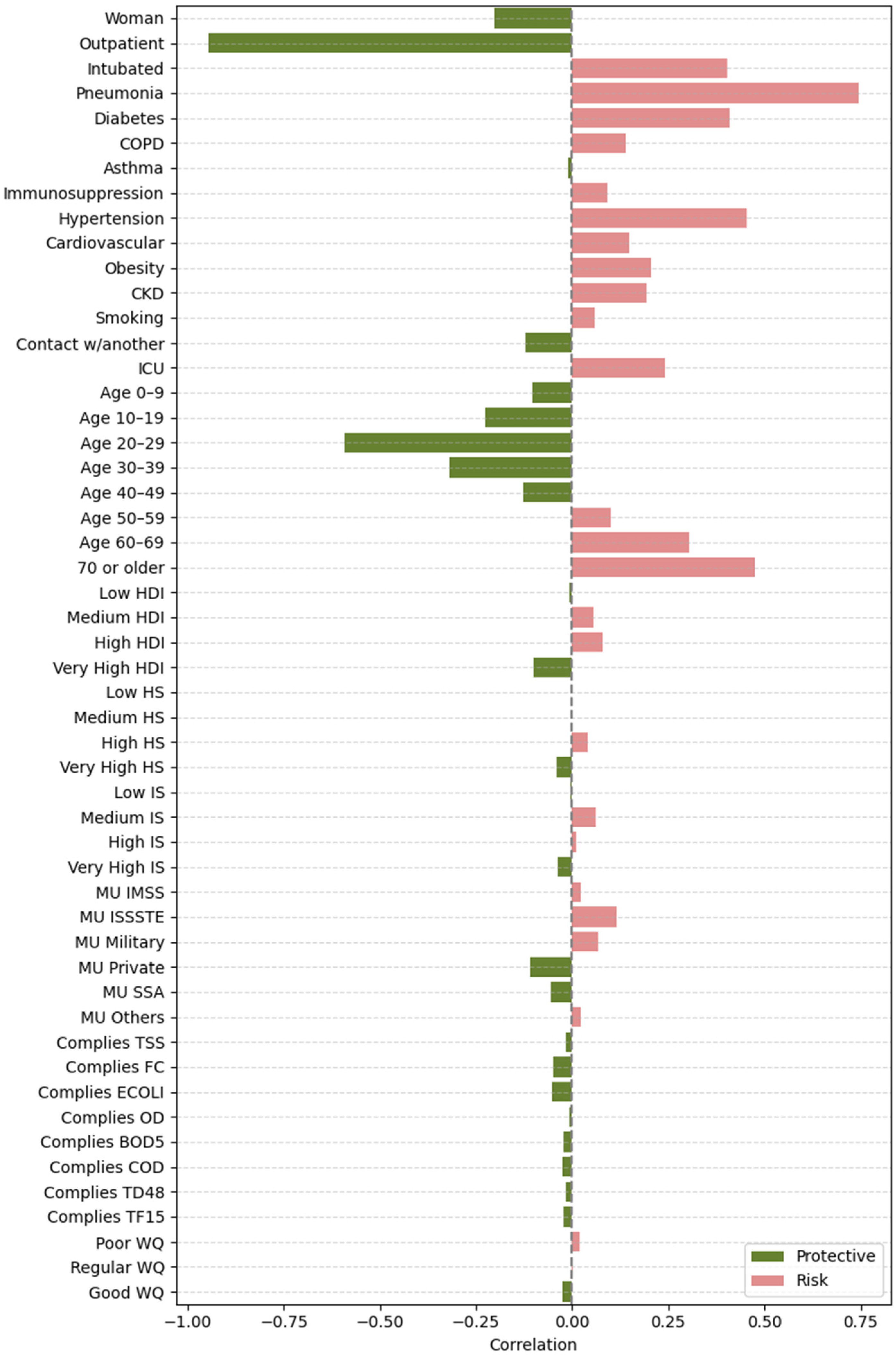
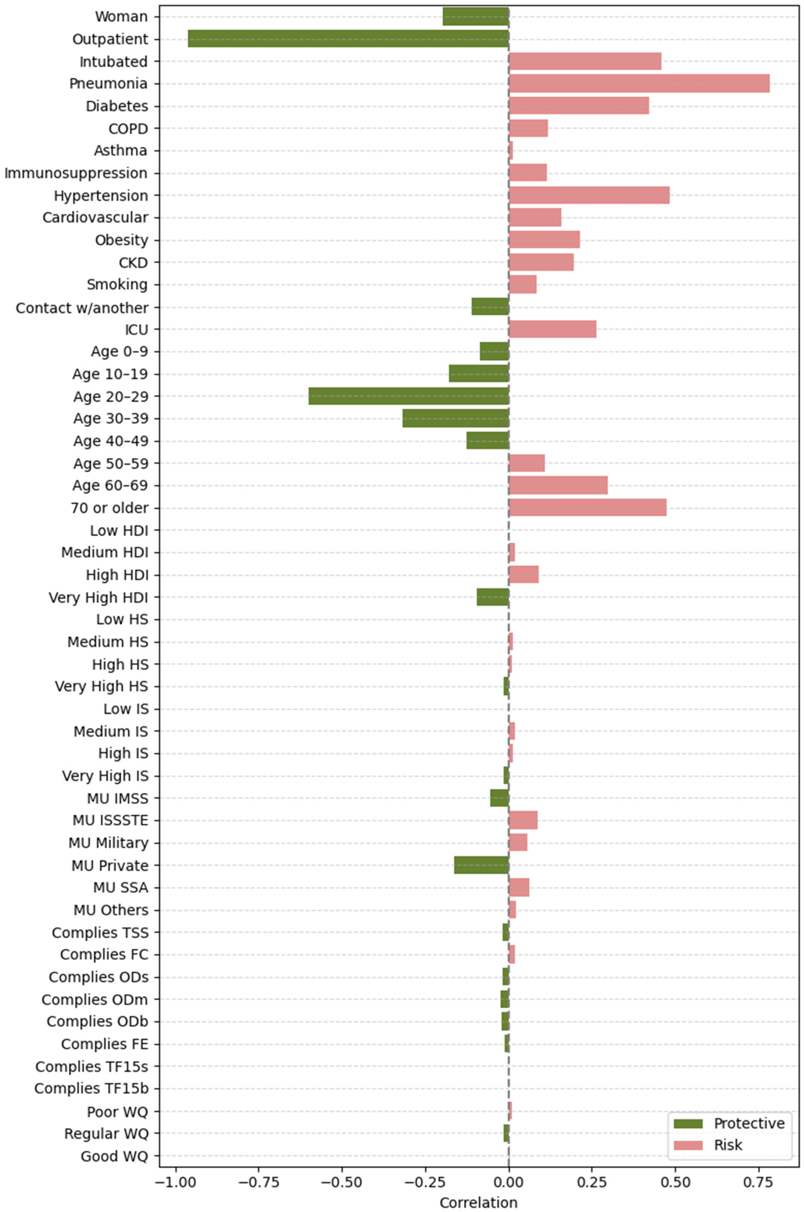
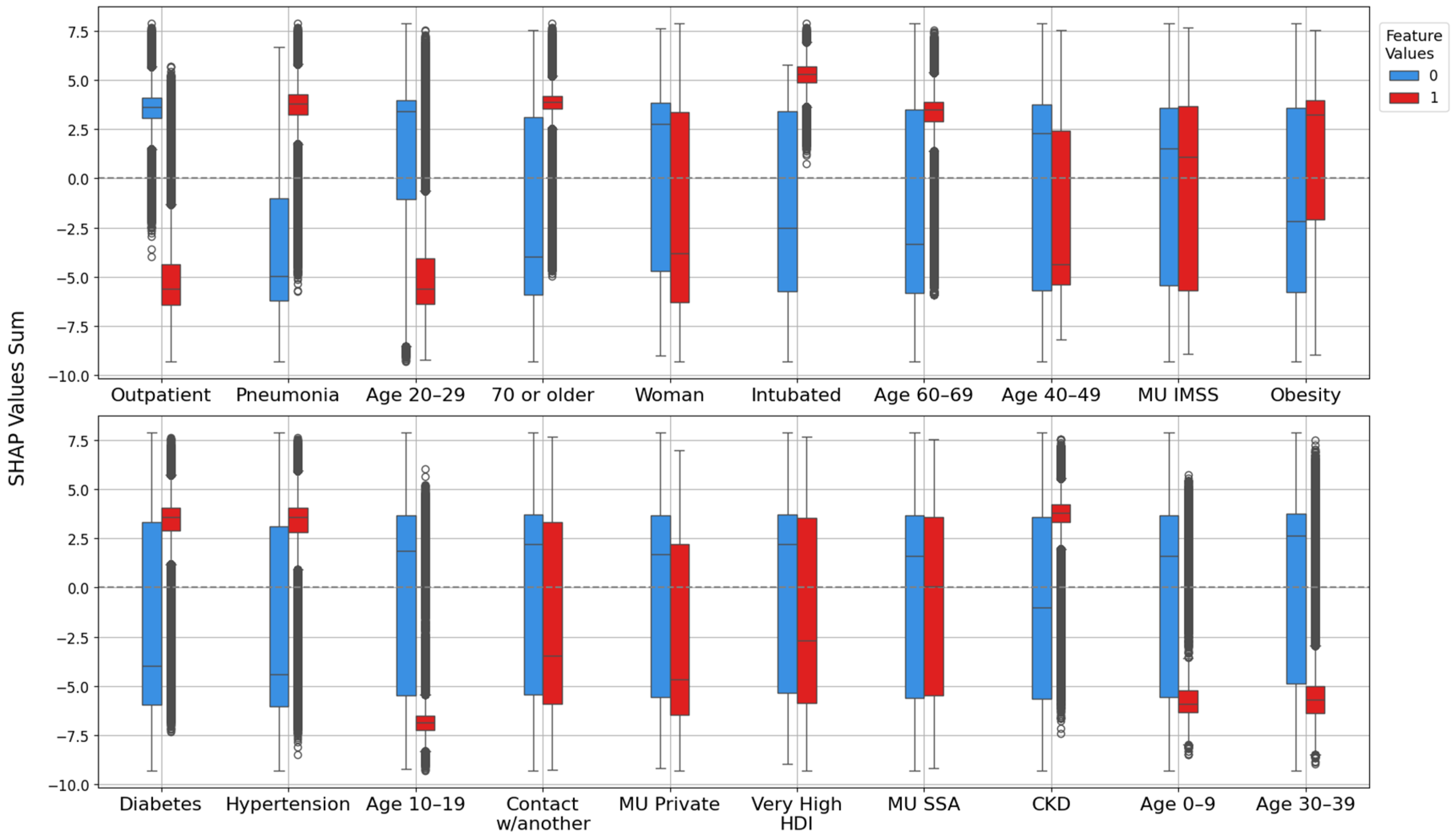
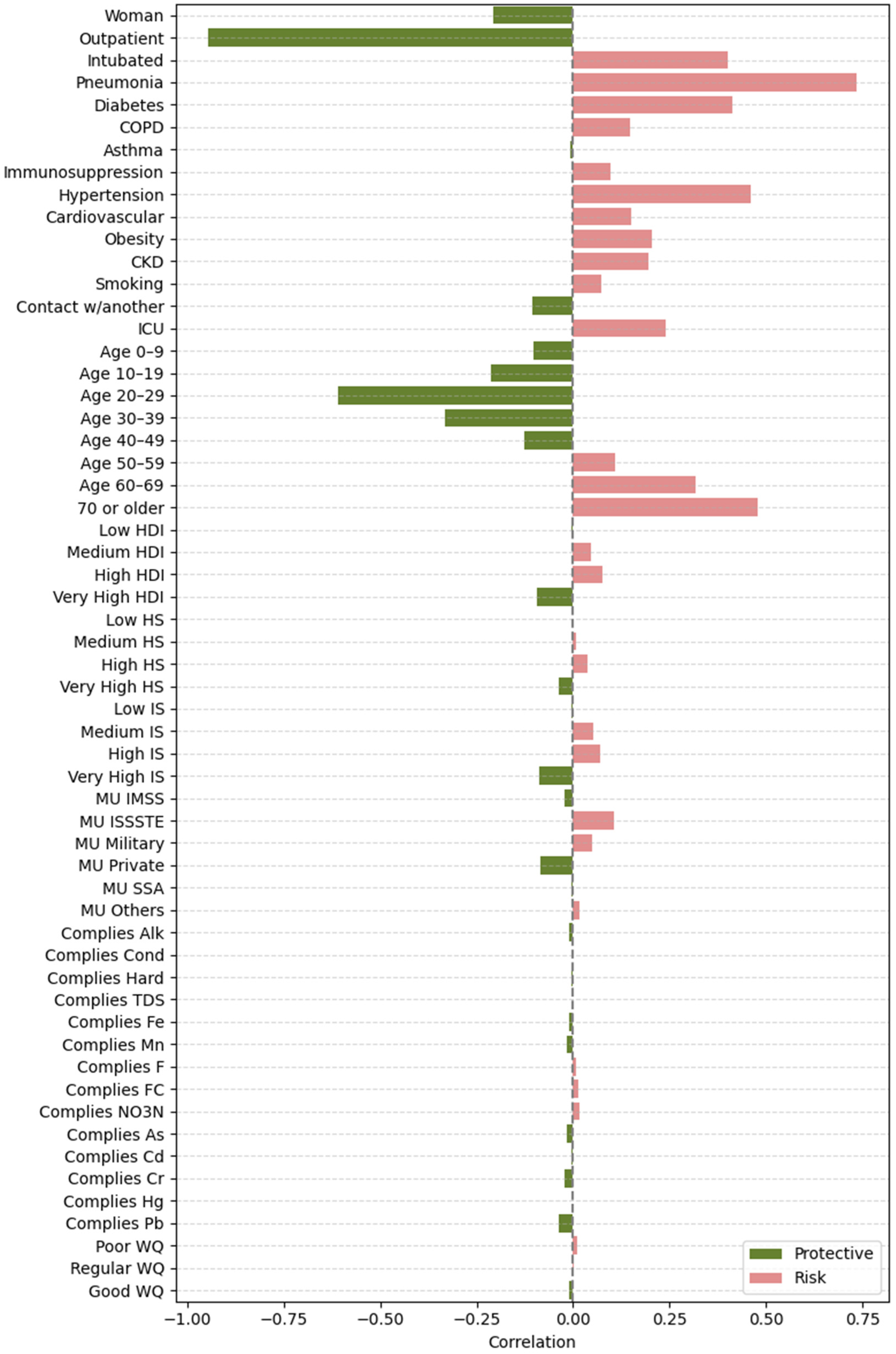
  • SHAP vs. target: Correlation between each feature’s SHAP values and patient outcomes. This analysis highlights whether higher SHAP values for a feature are associated with increased or decreased mortality risk.
  • Feature vs. SHAP: Correlation between binary feature values and the aggregated SHAP values: individual SHAP values provided a weighted measure of feature importance. Positive correlations indicated risk factors; negative correlations indicated protective factors.

2.5. XGBoost Models Interpretation Using Tree-Related Metrics

XGBoost provides internal metrics (gain, cover, and weight) that reveal the structural importance of features. The top 20 features based on these metrics were identified for each model. Notably, this threshold differs from that used with SHAP. SHAP captures nuanced interactions at the instance level, while tree-based metrics reflect structural influence during training. A narrower threshold was applied to the tree metrics to focus on consistently influential variables.
By integrating SHAP importance, point-biserial correlation, and XGBoost’s internal metrics, a robust and triangulated interpretation of feature importance was achieved, enhancing the reliability of the analysis.

3. Results

The following subsections present the training results of the XGBoost models, evaluate their performance on test datasets, and analyze feature importance using SHAP and XGBoost metrics. The four datasets (groundwater, lentic, lotic, and coastal), which integrate clinical, socioeconomic, and water quality variables, along with Python notebooks for each dataset documenting the implemented methodology, are available at the Zenodo web repository [31]. All experiments were conducted on a personal computer with an Intel(R) Core (TM) i7-11800H CPU (with 8 cores and 16 threads), an NVIDIA GeForce RTX 3060 Laptop GPU, and 16 GB of RAM.
Individual water quality contaminants are labeled with the prefix Complies_, which indicates whether each pollutant meets national environmental standards (e.g., Complies_Mn, Complies_As). While this prefix is retained in figures to match variable names, it is omitted in the text and tables to improve readability and fluency.

3.1. XGBoost Model Performance

The first section of Table 3 summarizes the average training and validation metrics for the XGBoost models applied to the groundwater, lentic, lotic, and coastal datasets. Each dataset was partitioned into multiple balanced subsets or splits, with one model trained per each. Evaluation metrics include accuracy, precision, recall, F1 Score, and MCC. The F1 Score and MCC provide comprehensive assessments integrating precision, recall, and class balance. All models achieved excellent performance with no signs of overfitting. Dataset-specific results:
  • Groundwater: The F1 Score values were 0.971 (±5.0 × 10⁻⁴) for training and 0.970 (±1.1 × 10⁻³) for testing. MCC values were 0.942 (±1.0 × 10⁻³) and 0.940 (±2.2 × 10⁻³), respectively.
  • Lentic: The F1 Score values were 0.973 (±3.0 × 10⁻⁴) for training and 0.972 (±5.0 × 10⁻⁴) for testing. MCC values were 0.946 (±5.0 × 10⁻⁴) and 0.944 (±1.0 × 10⁻³), respectively.
  • Lotic: The F1 Score values were 0.972 (±3.0 × 10⁻⁴) for training and 0.972 (±3.0 × 10⁻⁴) for testing. MCC values were 0.944 (±6.0 × 10⁻⁴) and 0.943 (±8.0 × 10⁻⁴).
  • Coastal: The F1 Score values were 0.979 (±3.0 × 10⁻⁴) for training and 0.978 (±4.0 × 10⁻⁴) for testing. MCC values were 0.958 (±6.0 × 10⁻⁴) and 0.956 (±8.0 × 10⁻⁴).
Table 3. Average performance metrics and most frequently selected hyperparameter values for XGBoost models across different datasets.
MetricGroundwaterLenticLoticCoastal
(A) Mean ( ± standard deviation) performance metrics for XGBoost models across different datasets:
Training accuracy0.971 ± 5.16 × 10−40.973 ± 2.78 × 10−40.972 ± 3.21 × 10−40.979 ± 3.21 × 10⁻⁴
Testing accuracy0.970 ± 1.143 × 10−30.972 ± 5.08 × 10−40.972 ± 3.16 × 10−40.978 ± 3.94 × 10⁻⁴
Training precision0.968 ± 8.99 × 10−40.970 ± 4.68 × 10−40.969 ± 4.35 × 10−40.973 ± 4.98 × 10⁻⁴
Testing precision0.968 ± 2.13 × 10−30.970 ± 9.13 × 10−40.968 ± 6.59 × 10−40.973 ± 7.03 × 10⁻⁴
Training recall0.974 ± 3.65 × 10−40.976 ± 1.94 × 10−40.976 ± 3.44 × 10−40.985 ± 3.12 × 10⁻⁴
Testing recall0.972 ± 6.77 × 10−40.975 ± 2.82 × 10−40.975 ± 2.05 × 10−40.983 ± 2.48 × 10⁻⁴
Training F1 score0.971 ± 5.01 × 10−40.973 ± 2.69 × 10−40.972 ± 2.98 × 10−40.979 ± 3.13 × 10⁻⁴
Testing F1 score0.970 ± 1.105 × 10−30.972 ± 4.88 × 10−40.972 ± 3.4 × 10−40.978 ± 3.8 × 10⁻⁴
Training MCC0.942 ± 1.014 × 10−30.946 ± 5.47 × 10−40.944 ± 5.78 × 10−40.958 ± 6.36 × 10⁻⁴
Testing MCC0.940 ± 2.237 × 10−30.944 ± 9.94 × 10−40.943 ± 8.02 × 10−40.956 ± 7.73 × 10⁻⁴
(B) Most frequently selected hyperparameter values for XGBoost models across different datasets:
max_depth8 (37%), 4 (24%), 10 (17%)4 (33%), 3 (23%), 7 (16%)6 (25%), 9 (22%), 5 (22%)3 (74%), 4 (12%), 6 (6%)
mid_child_weight6 (41%), 5 (37%), 4 (10%)4 (33%), 3 (26%), 6 (23%)3 (35%), 6 (32%), 4 (22%)4 (42%), 5 (33%), 3 (12%)
gamma0.0 (37%), 0.1 (24%), 0.3 (13%)0.0 (33%), 0.2 (30%), 0.4 (13%)0.0 (38%), 0.1 (25%), 0.2 (22%)0.2 (33%), 0.5 (21%), 0.4 (15%)
colsample_bytree0.7 (37%), 1.0 (31%), 0.8 (13%)1.0 (36%), 0.4 (23%), 0.3 (13%)1.0 (45%), 0.6 (19%), 5 (16%)0.6 (24%), 0.3 (24%), 0.5 (21%)
subsample0.7 (82%), 1.0 (13%), 0.8 (3%)1.0 (70%), 0.8 (10%), 0.7 (10%)1.0 (64%), 0.9 (25%), 0.8 (6%)1.0 (63%), 0.9 (21%), 0.8 (6%)
n_estimators100 (75%), 50 (13%), 150 (10%)100 (83%), 150 (13%), 50 (3%)100 (90%), 150 (9%)100 (54%), 50 (27%), 150 (18%)
reg_lambda0.5 (55%), 0.4 (17%), 0.8 (10%)0.6 (43%), 1.0 (16%), 0.7 (13%)1.0 (51%), 0.9 (12%), 0.5 (12%)1.0 (42%), 0.9 (15%), 0.4 (12%)
This consistently high performance across datasets with minimal variance suggests robust predictive capability and good generalization to unseen data.
The second section of Table 3 presents the most frequently selected hyperparameter values for each dataset, obtained using a grid search with five-fold stratified cross-validation. For example, in the groundwater dataset, the most common values were: max_depth: 8 (37% of models), 4 (24%), 10 (17%); min_child_weight: 6 (41%), 5 (37%), 4 (10%); gamma: 0.0 (37%); colsample_by_tree: 0.7 (37%); subsample: 0.7 (82%); n_estimators: 100 (75%); regularization_lambda: 0.5 (55%).

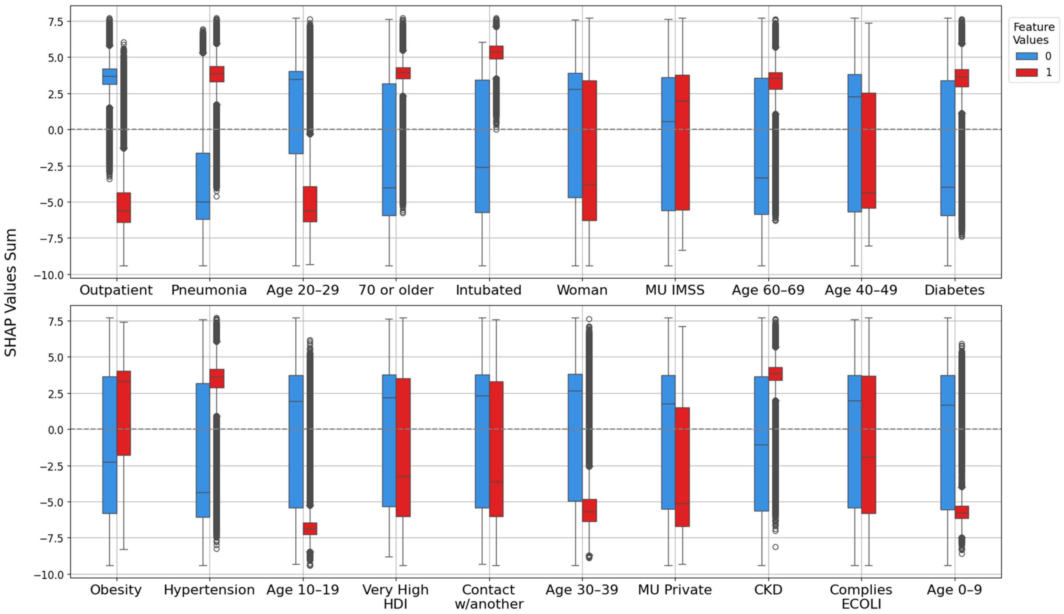
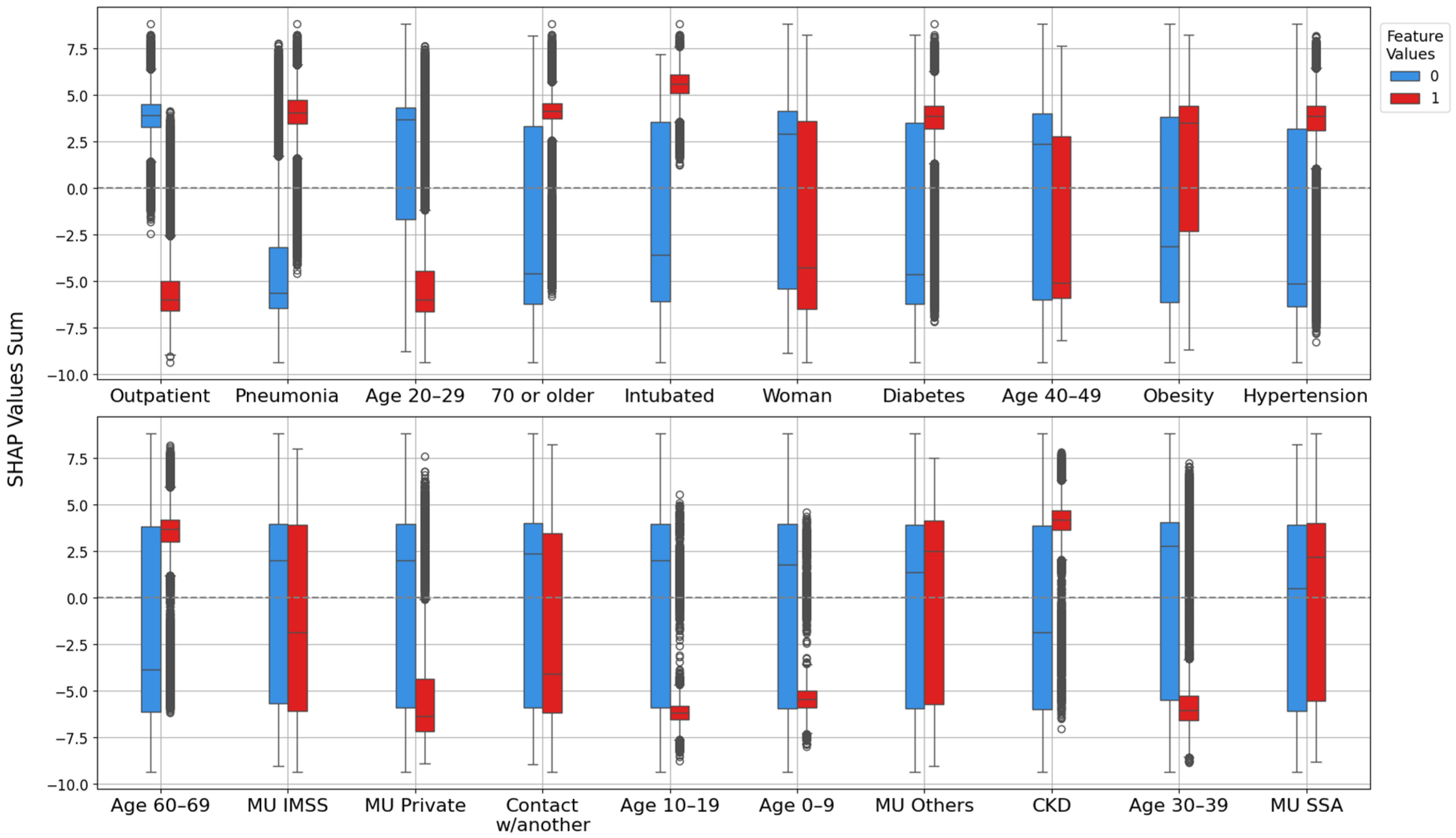
3.2. Model Explanation with SHAP Values

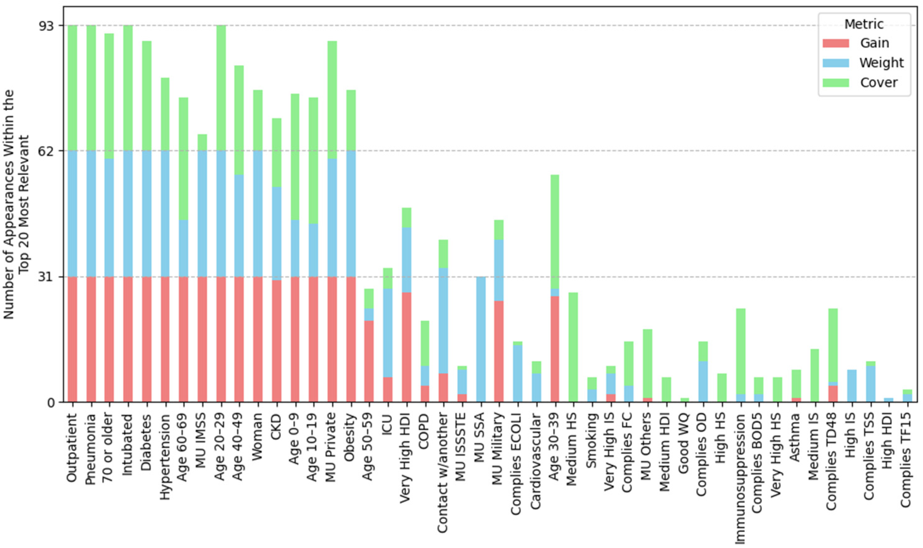
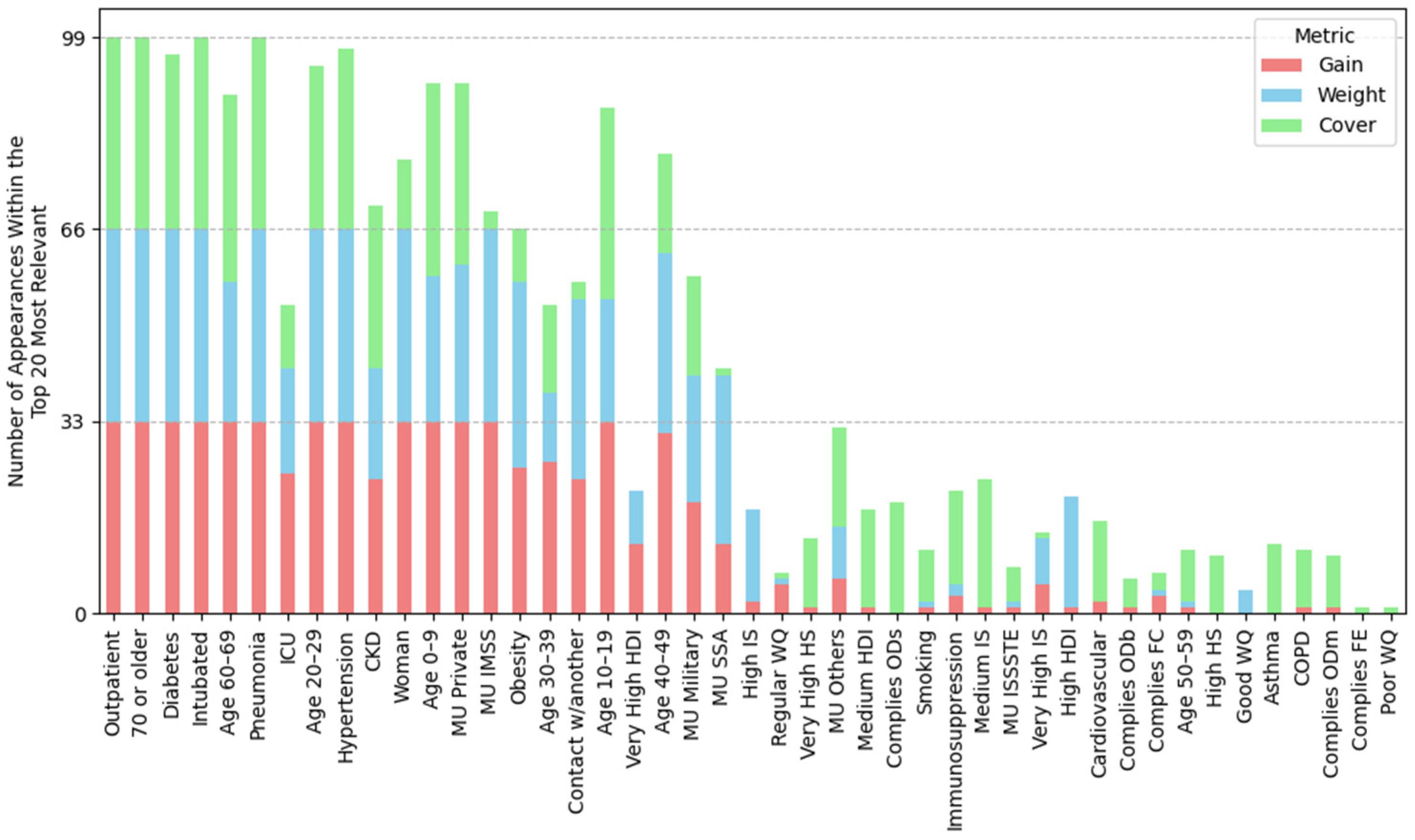
3.2.1. Feature Importance Analysis via SHAP Rankings Across All Splits

SHAP summary plots were generated for each model, ranking the top 30 most influential variables. Figure 4 presents a heatmap of feature rankings for the groundwater dataset, where the top eight variables, in descending order, were outpatient status, pneumonia, age groups 20–29 and 70+ years old, female sex, intubation, and ages 40–49 and 60–69 years old. Figure A1, Figure A2 and Figure A3 show heatmaps for the lentic, lotic, and coastal datasets, respectively, revealing similar patterns across datasets. In the coastal dataset, hypertension comorbidity replaces age 60–69 years old among the top-ranked variables.
Figure 5 presents a bar plot indicating the frequency of each variable’s ranking in the top 30 across all splits of the groundwater dataset. In addition to the key variables mentioned above, six others consistently appeared: medical care in IMSS units (MU IMSS), obesity, diabetes, hypertension, age 10–19 years old, and contact with a positive case. Figure A4, Figure A5 and Figure A6 illustrate similar distributions for the lentic, lotic, and coastal datasets, respectively, highlighting significant variations in feature rankings.
SHAP summary plots indicate whether a variable is “on” or “off”, but their interpretation as risk or protective factors is not always straightforward. To better illustrate SHAP value distributions, boxplots were generated for each feature. Figure 6 shows the distribution of SHAP values for the top 20 ranked features, with “on” states in red and “off” states in blue. Positive SHAP values indicate a higher mortality risk, while negative values suggest survival likelihood.
Protective factors included outpatient status and younger age groups (0–9, 10–19, 20–29, and 30–39 years old), while risk factors included pneumonia, age 70+ years old, intubation, ages 60–69 years old, diabetes, hypertension, and chronic kidney disease (CKD). Female sex showed a mild protective effect.
Figure A7, Figure A8 and Figure A9 present box plots for other datasets. Private medical care showed a mild protective effect in the lentic and coastal datasets. Notably, in the lentic dataset (Figure A7), water quality indicators (ODb, COD, and ‘good water quality’) were prominent, though their roles as risk or protective factors remain unclear. Similarly, in the lotic dataset (Figure A8), the ‘very high HDI’ socioeconomic condition and compliance with ECOLI standards were significant, but their exact influence is undefined.

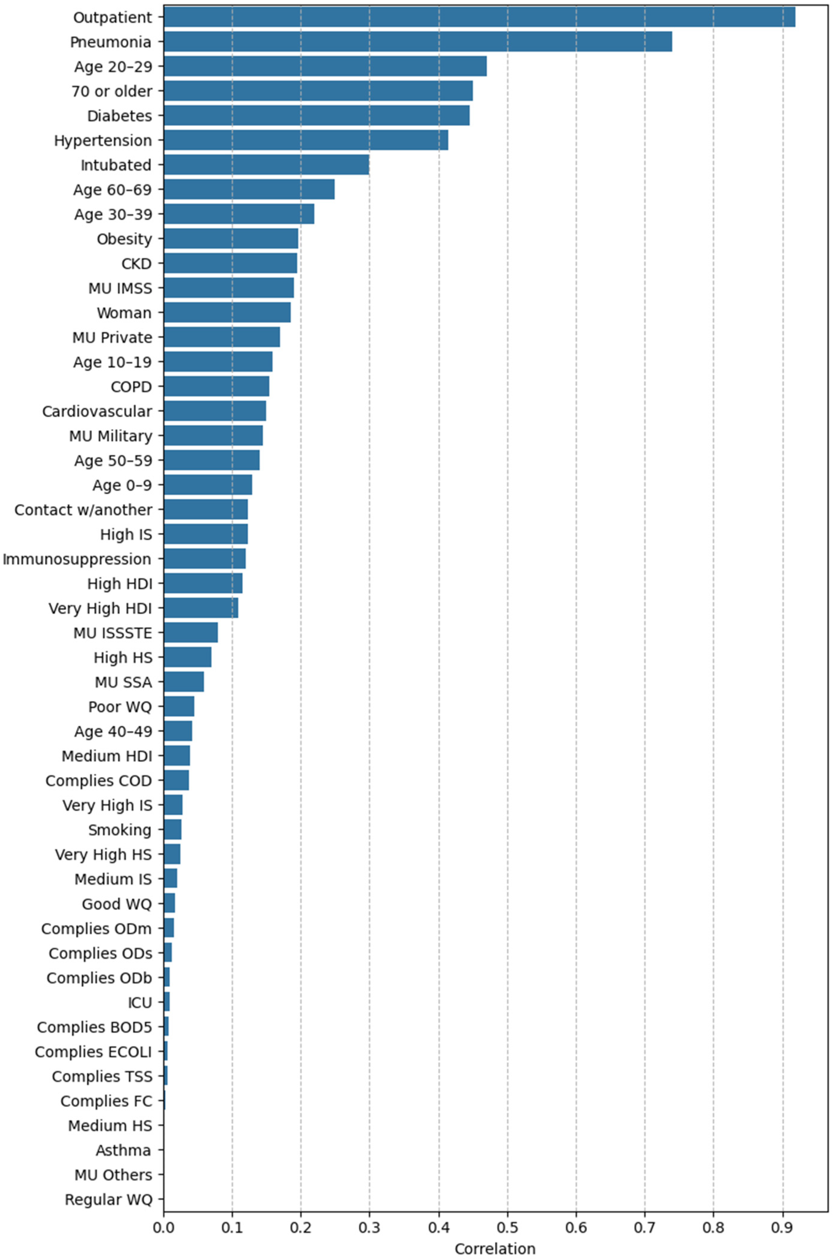
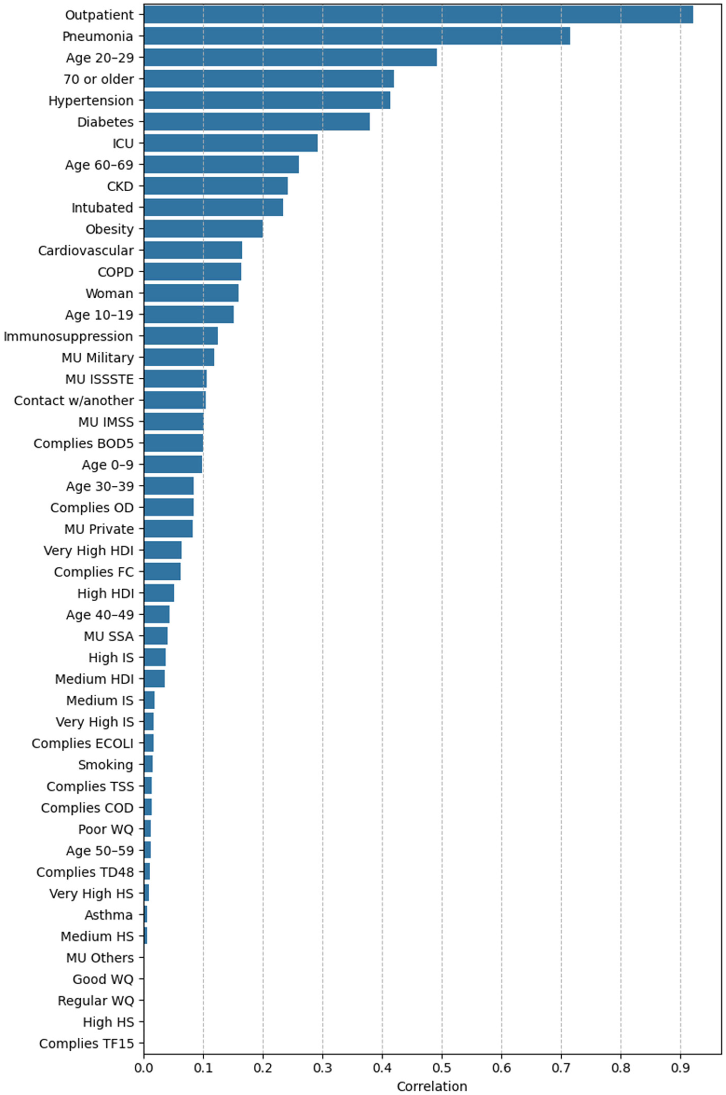
3.2.2. Feature Importance via Point-Biserial Correlation Across All Splits

The point-biserial correlation between SHAP values of each feature and patient survival status identified key predictors of mortality. Figure 7 shows the absolute correlation values, where higher values indicate stronger associations. Notably, key variables included outpatient status, pneumonia, age 20–29, hypertension, age 70+, diabetes, ages 60–69 and 30–39, ICU admission, intubation, CKD, and obesity, all show strong correlations. Similar patterns are seen in Figure A10, Figure A11 and Figure A12 for other datasets.
Figure 8 shows the relationship between the absolute point-biserial correlation coefficients (|r|) of SHAP values and the binary outcome (survival status), along with the corresponding statistical significance (−log10(p value)) for each feature across the four datasets analyzed. Most correlations exhibit high statistical significance (p < 0.05), as indicated by their positions above the red-dotted horizontal line. However, only a smaller subset of features shows both statistical significance and practical relevance, defined by correlation thresholds of |r| ≥ 0.1 (minimum), ≥0.2 (moderate), and ≥0.4 (high), marked by vertical dashed lines.
Features such as outpatient, pneumonia, and age 20–29 years old consistently demonstrate strong associations (|r| > 0.4) across all datasets, highlighting their robust predictive power. In contrast, a set of variables showed moderate practical relevance (0.2 ≤ |r| < 0.4), such as hypertension, diabetes, and age 70 years or older, which may reflect the epidemiological stability of clinical risk factors. At the lower end of the practical relevance spectrum (|r| < 0.1), many features remain statistically significant but show weak associations. These included various water quality indicators such as FC, ODb, and ECOLI, as well as some socioeconomic attributes such as medium IS, very high HS, and MU others. This analysis emphasizes the consistency of top-ranked clinical predictors across datasets, but the heterogeneity of socioeconomic and environmental features suggests that the impact of non-clinical factors may be more context-dependent.
Further analysis correlated binary feature values with aggregated SHAP scores to assess mortality risk. Positive correlations indicate risk factors, while negative correlations suggest protective effects. Figure 9 highlights outpatient status and age 20–29 as strong protective factors, while intubation, pneumonia, diabetes, hypertension, ICU admission, and older age were significant risk factors. These results align with SHAP rankings, reinforcing identified risk and protective factors. Figure A13, Figure A14 and Figure A15 show similar patterns across other datasets. Smoking and all comorbidities (except asthma) were risk factors. Being over 50 increased mortality risk, while residing in a municipality with a very high Human Development Index (HDI) was protective. Care in private medical units was consistently associated with a protective effect.
The statistical significance of the correlation between binary features and aggregated SHAP scores was also assessed. Figure 10 displays the relationship between the absolute point-biserial correlation coefficients (|r|) and the statistical significance (−log10(p value)) of the SHAP values for each feature across the four datasets analyzed. As shown, most variables lie well above the significance threshold (p < 0.05, red-dotted line), reflecting high statistical power. However, practical relevance, indicated by the correlation size thresholds |r| ≥ 0.1 (minimal), ≥0.2 (moderate), and ≥0.4 (high), varies substantially among features.
A subset of variables (outpatient, pneumonia, and age 20–29 years old) shows both high statistical significance (−log10(p) > 300) and practical relevance (|r| > 0.4 across all datasets). These features consistently stand out as robust and highly informative predictors of mortality.
Beyond this group, several variables fall within the moderate relevance range (0.2 ≤ |r| < 0.4), including age groups such as age 60–69 years old, clinical factors such as intubated and ICU, and chronic conditions such as CKD and obesity. These features show consistent associations with patient outcomes, though with lower correlation sizes than the top predictors.
At the lower end of the relevance spectrum, certain variables remain statistically significant despite smaller effect sizes. These include smoking, high HDI, and various water quality indicators (e.g., FC, poor and regular WQ). While their practical impact appears limited (|r| < 0.1), their significance suggests that they may still contribute marginally in specific contexts or subpopulations.

3.3. Feature Importance via XGBoost Tree-Related Metrics

Figure 11 presents a stacked bar plot showing how often each variable was ranked among the top 20 most important features according to different XGBoost tree-building metrics (gain, weight, and cover). Figure A16, Figure A17 and Figure A18 present bar plots for other datasets, showing similar feature importance patterns.

3.4. Condensed Analysis of Feature Importance Across All Datasets

3.4.1. Feature Importance by Position Rank

Feature importance analysis across all datasets revealed strong agreement among the methods used (SHAP, point-biserial correlation, and XGBoost metrics). Features with high point-biserial correlations were generally ranked as “highest” or “high” importance by SHAP (Table 4). Similarly, the top 20 variables identified by XGBoost often matched those from the other methods, although some were classified as “medium-high” importance.
Table 4, section A, summarizes SHAP-derived feature importance across the four datasets using four thresholds based on mean ranking positions and their variability (i.e., positional shifts among variables) across splits. These rankings are based on the SHAP values of the top 30 most important variables for each dataset.
In general, features classified as “highest importance” (1st to 8th place in Table 4) exhibited stable rankings across datasets, indicating a strong influence on mortality. These include outpatient status, pneumonia, age (70+, 20–29, 40–49, and 60–69), female sex, and intubation.
The “high importance” features (9th to 14th place), consistent across most datasets, included obesity, diabetes, hypertension, age 10–19, and MU IMSS.
Although “mid-high importance” features (15th–19th place) varied considerably in ranking, age groups 0–9 and 30–39 years old and chronic kidney disease (CKD) remained consistent across most datasets. Contact with an infected person was highly important in the groundwater and lentic datasets but ranked only mid-high important in the other two datasets. The lentic dataset stood out for the prominence of ODb, COD pollution levels, and good water quality, while the lotic dataset highlighted the very high HDI socioeconomic indicator.
Finally, features categorized as “mid-importance” (20th place and below) showed the greatest variability across datasets, suggesting a weaker correlation with mortality. Care in private and SSA medical units was identified as a medium-importance factor, along with several water quality parameters: Mn and hardness in groundwater; ODs in lentic systems; OD, ECOLI, FC, and BOD5 in lotic systems; and FC in coastal areas. High and very high HDI indexes and IS subindex were also medium-importance socioeconomic factors in coastal waters.

3.4.2. Water Quality and Socioeconomic Feature Importance

Our analysis revealed a potential association between water contaminants and COVID-19 mortality (Table 4, Section B). Among the top 30 influential variables, both overall water quality categories (good, normal, and poor) and specific pollutants frequently appeared, including (i) manganese (Mn), hardness, and fluoride (F) in the groundwater dataset; (ii) background dissolved oxygen (ODb) and chemical oxygen demand (COD) in the lentic dataset; (iii) dissolved oxygen (OD), fecal coliforms (FC), and Escherichia coli (ECOLI) in the lotic dataset; and (iv) fecal coliforms and dissolved oxygen levels in the coastal dataset.
While causality cannot be established, the consistent presence of water-related variables among the top 30 suggests a potential link between environmental exposure and health outcomes, warranting further investigation.
Socioeconomic conditions also emerged as relevant predictors. The prominence of high and very high levels in our models suggests a potential association between higher socioeconomic status and a reduced risk of COVID-19 mortality.

4. Discussion

4.1. Clinical and Demographic Factors

The identification of older age, pneumonia, and intubation as the most critical risk factors for COVID-19 mortality aligns with previous findings by Carvantes et al. [11]. While numerous studies e.g., [3,4,5,6,7,8,9,10,11,12,13] have identified older age as a risk factor, our analysis specifically highlights individuals aged 50 years and older as being at higher risk, while younger age groups appear protective. The protective effects of outpatient status and younger age are consistent with the current understanding of COVID-19 progression. Although the protective role of the female sex was less pronounced, it aligns with some studies suggesting potential gender differences in COVID-19 outcomes.
The identification of diabetes and hypertension as high-risk factors corroborates previous research by Datta et al. [6] and Carvantes et al. [11], which associated these comorbidities with increased COVID-19 mortality. While the IMSS medical unit was identified as an important factor, our findings do not fully replicate those of Carvantes et al. [11], who reported IMSS as a high-risk factor. Notably, age 10–19 years old was identified as a strong protective factor.
CKD emerged as a moderate-to-high risk factor, consistent with findings by Wollenstein-Betech et al. [3], Datta et al. [6], and Rojas-García et al. [7]. Additionally, younger age groups (0–9 and 30–39 years) were identified as protective factors of moderate-to-high importance.

4.2. Environmental Factors

The presence of water quality contaminants among the top 30 influential factors suggests a potential association between environmental conditions and health outcomes, warranting further investigation. This raises questions about indirect effects, such as the impact of water quality on overall health and infection susceptibility, or the presence of shared environmental risk factors. Future research should explore these relationships in more detail.

4.3. Socioeconomic Factors

Very high levels of the Human Development Index (HDI) and its health (HS) and income (IS) subindexes appeared protective against COVID-19 mortality, while lower levels were associated with increased risk. Our findings align with global trends [12], where higher HDI was associated with lower mortality. However, as our study focuses on specific regions, this association may reflect complex interactions between socioeconomic status, access to healthcare, and other regional factors. As reported by Carvantes et al. [11], residing in a municipality with a very low HDI was a risk factor, indirectly supporting our findings by highlighting the role of socioeconomic context. Similarly, Chu et al. [13] highlighted the influence of education, often correlated with HDI, on COVID-19 hospitalization rates, highlighting the complex interaction between socioeconomic status and health outcomes.
While socioeconomic conditions frequently appeared as relevant variables in predictive models, their inclusion does not necessarily imply direct causality. Factors such as healthcare access, medical service quality, and other socioeconomic conditions could influence this association. Therefore, further research is needed to elucidate these complex relationships.

4.4. Feature Importance Methodologies: A Comparative Analysis

Although the three feature importance methods (SHAP, point-biserial correlation, and XGBoost metrics) generally agreed, some discrepancies were observed. For instance, in the groundwater dataset, cardiovascular disease was ranked differently between SHAP and point-biserial correlation (Figure 4 and Figure 7). Despite similar point-biserial correlations, age 10–19 appeared in the SHAP top 30 for all 29 splits, whereas cardiovascular disease appeared in only 3 splits.
This discrepancy arises because SHAP values distribute the contribution of correlated features across multiple variables rather than assigning all importance to a single predictor. Unlike traditional feature importance measures, which may attribute zero importance to collinear variables, SHAP ensures that each correlated feature retains a proportional share of its predictive contribution.
Furthermore, tree-based models such as XGBoost capture complex feature interactions, meaning a variable’s relevance depends on how it interacts with others within each dataset split. SHAP values reflect these interactions, sometimes elevating the importance of a feature that is not highly predictive on its own but plays a crucial role in combination with others. Consequently, SHAP rankings offer a more comprehensive view of feature importance across multiple dataset partitions, while correlation with the target variable remains necessary but insufficient for consistent feature selection. The observed variability in rankings reflects both the model’s flexibility in selecting among correlated predictors and the local versus global nature of SHAP explanations.
Moreover, while this study focused on clinical, socioeconomic, and environmental factors, we acknowledge that other structural and behavioral factors may also influence the patterns of SARS-CoV-2 transmission and lethality. For instance, previous studies have highlighted the important role of school operations during the pandemic, particularly in the European context. In Italy, the reopening of schools in 2020 was shown to have a significant impact on the growth rate of new COVID-19 cases, underscoring the importance of including educational environments in future epidemiological models and public health strategies [32,33]. These aspects represent a relevant avenue for future studies aiming for a more comprehensive understanding of pandemic determinants.

4.5. Complementary Analysis: Evaluating Pre-Infection Predictors by Excluding Clinical Outcome Variables

We conducted a complementary analysis to better assess the predictive contribution of pre-infection variables, particularly water quality parameters, by removing three clinical outcome features: outpatient, pneumonia, and intubated. These variables, which reflect symptom severity after infection, are among the strongest predictors of COVID-19 mortality and were expected to dominate model outputs.
We retrained the models from scratch using the same pipeline but excluded these three post-infection variables. As anticipated, the overall predictive performance declined substantially, with the F1 score and other evaluation metrics dropping from ~0.97 to a range between 0.83 and 0.86. This decrease underscores the strong predictive power of the excluded features but also provides an opportunity to examine the stability of pre-infection predictors in their absence.
To this end, we compared the absolute point-biserial correlations between SHAP values and each feature before and after exclusion.
The results showed that the relative importance of most water quality contaminants remained stable across all four datasets (groundwater, lentic, lotic, and coastal), with most correlation differences falling within ±0.05. A few contaminants showed modest increases in relevance, such as Mn, Fe, and Alk in groundwater, and ODm, ODb, and ECOLI in lentic waters, suggesting a slight enhancement in their predictive contribution when dominant clinical features were excluded. Other datasets (lotic and coastal) exhibited mixed but generally minor shifts in importance.
Overall, this complementary analysis reinforces the robustness of the main findings by confirming that water quality contaminants retain their relevance even when high-impact post-infection variables are removed. At the same time, it highlights the inherent challenge of isolating weaker predictors in the presence of highly dominant clinical features.

5. Conclusions

This study investigated factors associated with COVID-19 mortality using machine learning models applied to four datasets of COVID-19-positive patients from municipalities with water quality monitoring sites across four water body types in Mexico (groundwater, lentic, lotic, and coastal).
The high predictive performance of XGBoost models underscores their potential utility in identifying individuals at increased risk of death. These models consistently achieved high performance across all datasets, with average F1 scores exceeding 0.97 and MCC values above 0.94. Feature importance analysis using SHAP scores, point-biserial correlation, and XGBoost metrics showed general agreement in identifying key factors.
Our findings confirm the significance of previously identified clinical and demographic risk factors, including older age (especially 50+ years old), pneumonia, intubation, diabetes, and hypertension. Younger age groups (0–9, 10–19, 20–29, and 30–39 years old) and outpatient status emerged as protective factors, while female sex showed a modest protective effect.
Importantly, this study also explored the potential influence of environmental and socioeconomic factors on COVID-19 mortality. The consistent presence of water quality contaminants (e.g., manganese, hardness, fluoride, dissolved oxygen, and fecal coliforms) among the top 30 influencing variables suggests a possible link between these factors and health outcomes. While causality cannot be inferred, these findings warrant further research into how environmental exposures influence COVID-19 susceptibility.
Similarly, the association between higher levels of the Human Development Index and its health and income subindexes with lower mortality risk, along with the increased risk linked to lower levels, highlights the potential role of socioeconomic disparities. However, further research is needed to disentangle the complex interactions between socioeconomic status, healthcare access, and regional factors that may contribute to this association.
This study addresses health and socioeconomic disparities while accounting for environmental factors through advanced data analytics and machine learning, aiming to improve healthcare strategies and reduce health disparities.

Author Contributions

Conceptualization, L.D.-G., J.C.P.-S. and N.L.; methodology, L.D.-G. and Y.S.T.-C.; software, Y.S.T.-C.; validation, Y.S.T.-C.; investigation, L.D.-G., Y.S.T.-C., J.C.P.-S. and N.L.; data curation, Y.S.T.-C.; writing—original draft preparation, L.D.-G.; writing—review and editing, Y.S.T.-C., J.C.P.-S. and N.L.; visualization, Y.S.T.-C.; supervision, L.D.-G., J.C.P.-S. and N.L. All authors have read and agreed to the published version of the manuscript.

Funding

This research received no external funding.

Data Availability Statement

The datasets and Python notebooks used in this work are available at the web repository: https://doi.org/10.5281/zenodo.14931751 (accessed on 11 June 2025).

Acknowledgments

We thank the anonymous reviewers for their valuable comments and the editor, Thanakorn Prasansri, for handling the editorial process. The first author acknowledges the sabbatical scholarship granted by Secretaría de Ciencia, Humanidades, Tecnología e Innovación (SECIHTI) and the institutional support provided by Instituto Nacional de Astrofísica, Óptica y Electrónica (INAOE) during the development of this work.

Conflicts of Interest

The authors declare that they have no known competing financial interests or personal relationships that could have appeared to influence the work reported in this paper.

Appendix A

This appendix provides more details on the methodology and results of the study. Table A1 summarizes water quality limits according to Mexican regulations. Figure A1, Figure A2, Figure A3, Figure A4, Figure A5, Figure A6, Figure A7, Figure A8, Figure A9, Figure A10, Figure A11, Figure A12, Figure A13, Figure A14, Figure A15, Figure A16, Figure A17 and Figure A18 present feature importance analysis, including SHAP value distributions, correlations, and model metrics for groundwater, lentic, lotic, and coastal datasets.
Table A1. Summary of permissible water quality limits for human use and consumption as reported by CONAGUA, according to Mexican Official Norm NOM-127-SSA1-2021 [20,21].
Pollutant ParameterUnitsLimits for Good Water QualityWater Quality Classification for Non-Compliance
(a) Groundwater
Alkalinity (Alk)mg CaCO3/L20 ≤ Alk ≤ 400Regular
Electrical conductivity (Cond)μS/cmCond ≤ 2000Regular
Total hardness (Hard)mg CaCO3/LHard ≤ 500Regular
Total dissolved solids (TDS)mg/LTDS ≤ 2000Regular
Iron (Fe)mg/LFe ≤ 0.30Regular
Manganese (Mn)mg/LMn ≤ 0.15Regular
Fluorides (F)mg/LF < 1.5Poor
Fecal coliforms (FC)NMP/100_mLFC ≤ 1000Poor
Nitrate-nitrogen (NO3-N)mg/LNO3-N ≤ 11Poor
Arsenic (As)mg/LAs ≤ 0.025Poor
Cadmium (Cd)mg/LCd ≤ 0.005Poor
Chromium (Cr)mg/LCr ≤ 0.05Poor
Mercury (Hg)mg/LHg ≤ 0.006Poor
Lead (Pb)mg/LPb ≤ 0.01Poor
(b) Lotic water
Total suspended solids (TSS)mg/LTSS ≤ 150Regular
Fecal coliforms (FC)NMP/100_mLFC ≤ 1000Regular
Escherichia coli (ECOLI)NMP/100 mlECOLI ≤ 850Regular
% oxygen demand saturation (OD%)% Saturation30 < OD% ≤ 130Regular
5-day biochemical oxygen demand (BOD5)mg/LBOD5 ≤ 30Poor
Chemical oxygen demand (COD)mg/LCOD ≤ 40Poor
Toxicity Daphnia Magna, 48 h (TD48)UTTD48 < 5Poor
Toxicity Vibrio Fischeri, 15 min (TF15)UTTF15 < 5Poor
(c) Lentic water
Total suspended solids (TSS)mg/LTSS ≤ 150Regular
Fecal coliforms (FC)NMP/100_mLFC ≤ 1000Regular
Escherichia soli (ECOLI)NMP/100 mlECOLI ≤ 850Regular
% OD at surface (ODs%)% Saturation30 < ODs% ≤ 130Regular
% OD at medium (ODm%)% Saturation30 < ODm% ≤ 130Regular
% OD at background (ODb%)% Saturation30 < ODb% ≤ 130Regular
BOD5mg/LBOD5 ≤ 30Poor
Chemical oxygen demand (COD)mg/LCOD > 40Poor
TD48 at surface (TD48s)UTTD48s < 5Poor
TD48 at background (TD48b)UTTD48b < 5Poor
TF15 at surface (TF15s)UTTF15s < 5Poor
TF15 at background (TF15b)UTTF15b < 5Poor
(d) Coastal water
Total suspended solids (TSS)mg/LTSS ≤ 150Regular
Fecal coliforms (FC)NMP/100_mLFC ≤ 1000Regular
% OD at surface (ODs%)% Saturation30 < ODs% ≤ 130Regular
% OD at medium (ODm%)% Saturation30 > ODm% ≤ 130Regular
% OD at background (ODb%)% Saturation30 > ODb% ≤ 130Regular
Fecal enterococci (FE)NMP/100 mlFE ≤ 200Poor
TF15 at surface (TF15s)UTTF15s < 5Poor
TF15 at background (TF15b)UTTF15b < 5Poor
Figure A1. Heatmap of SHAP summary plots rankings for the 30 splits of the lentic dataset. Blank spaces indicate that the feature was not ranked among the top 30 variables.
Make 07 00055 g0a1
Figure A2. Heatmap of SHAP summary plots rankings for the 31 splits of the lotic dataset. Blank spaces indicate that the feature was not ranked among the top 30 variables.
Make 07 00055 g0a2
Figure A3. Heatmap of SHAP summary plots rankings for the 33 splits of the coastal dataset. Blank spaces indicate that the feature was not ranked among the top 30 variables.
Make 07 00055 g0a3
Figure A4. Barplot showing the frequency of features ranked among the top 30 most important in each of the 30 splits of the lentic dataset.
Make 07 00055 g0a4
Figure A5. Barplot showing the frequency of features ranked among the top 30 most important in each of the 31 splits of the lotic dataset.
Make 07 00055 g0a5
Figure A6. Barplot showing the frequency of features ranked among the top 30 most important in each of the 33 splits of the coastal dataset.
Make 07 00055 g0a6
Figure A7. Boxplots illustrate the distribution of SHAP values of the top 20 most important features in the lentic dataset. Blue boxes represent the SHAP value range when a feature is “off”, while red boxes indicate the range when the feature is “on”, and black circle indicate outliers beyond the interquartile range.
Make 07 00055 g0a7
Figure A8. Boxplots illustrate the distribution of SHAP values of the top 20 most important features in the lotic dataset. Blue boxes represent the SHAP value range when a feature is “off”, while red boxes indicate the range when the feature is “on”, and black circle indicate outliers beyond the interquartile range.
Make 07 00055 g0a8
Figure A9. Boxplots illustrate the distribution of SHAP values of the top 20 most important features in the coastal dataset. Blue boxes represent the SHAP value range when a feature is “off”, while red boxes indicate the range when the feature is “on”, and black circle indicate outliers beyond the interquartile range.
Make 07 00055 g0a9
Figure A10. Barplot displays the absolute point-biserial correlation values of each feature in the lentic dataset, sorted in descending order.
Make 07 00055 g0a10
Figure A11. Barplot displays the absolute point-biserial correlation values of each feature in the lotic dataset, sorted in descending order.
Make 07 00055 g0a11
Figure A12. Barplot displays the absolute point-biserial correlation values of each feature in the coastal dataset, sorted in descending order.
Make 07 00055 g0a12
Figure A13. Barplot of point-biserial correlation values between each binary feature and aggregated SHAP values in the lentic dataset. A positive correlation indicates the feature acts as a risk factor for mortality, while a negative correlation suggests a protective effect.
Make 07 00055 g0a13
Figure A14. Barplot of point-biserial correlation values between each binary feature and aggregated SHAP values in the lotic dataset. A positive correlation indicates the feature acts as a risk factor for mortality, while a negative correlation suggests a protective effect.
Make 07 00055 g0a14
Figure A15. Barplot of point-biserial correlation values between each binary feature and aggregated SHAP values in the coastal dataset. A positive correlation indicates the feature acts as a risk factor for mortality, while a negative correlation suggests a protective effect.
Make 07 00055 g0a15
Figure A16. Stacked barplot showing the count of features ranked among the top 20 most important for each XGBoost tree-building metric across the 30 splits of the lentic dataset.
Make 07 00055 g0a16
Figure A17. Stacked barplot showing the count of features ranked among the top 20 most important for each XGBoost tree-building metric across the 31 splits of the lotic dataset.
Make 07 00055 g0a17
Figure A18. Stacked barplot showing the count of features ranked among the top 20 most important for each XGBoost tree-building metric across the 33 splits of the coastal dataset.
Make 07 00055 g0a18

References

  1. PAHO. WHO Characterizes COVID-19 as a Pandemic. Available online: https://www.paho.org/en/news/11-3-2020-who-characterizes-covid-19-pandemic (accessed on 25 April 2025).
  2. WHO. WHO Coronavirus (COVID-19) Dashboard. Available online: https://covid19.who.int/ (accessed on 25 April 2025).
  3. Wollenstein-Betech, S.; Cassandras, C.G.; Paschalidis, I.C. Personalized predictive models for symptomatic COVID-19 patients using basic preconditions: Hospitalizations, mortality, and the need for an ICU or ventilator. Int. J. Med. Inform. 2020, 142, 104258. [Google Scholar] [CrossRef] [PubMed]
  4. Khadem, H.; Nemat, H.; Eissa, M.R.; Elliott, J.; Benaissa, M. COVID-19 mortality risk assessments for individuals with and without diabetes mellitus: Machine learning models integrated with interpretation framework. Comput. Biol. Med. 2022, 144, 105361. [Google Scholar] [CrossRef] [PubMed]
  5. Barría-Sandoval, C.; Ferreira, G.; Espinoza Venegas, M.; Marchant, V. Interpretable machine learning for mortality modeling on patients with chronic diseases considering the COVID-19 pandemic in a region of Chile: A Shapley value based approach. Res. Stat. 2023, 1, 2240334. [Google Scholar] [CrossRef]
  6. Datta, D.; George Dalmida, S.; Martinez, L.; Newman, D.; Hashemi, J.; Khoshgoftaar, T.M.; Shorten, C.; Sareli, C.; Eckardt, P. Using machine learning to identify patient characteristics to predict mortality of in-patients with COVID-19 in south Florida. Front. Digit. Health 2023, 5, 1193467. [Google Scholar] [CrossRef] [PubMed]
  7. Rojas-García, M.; Vázquez, B.; Torres-Poveda, K.; Madrid-Marina, V. Lethality risk markers by sex and age-group for COVID-19 in Mexico: A cross-sectional study based on machine learning approach. BMC Infect. Dis. 2023, 23, 18. [Google Scholar] [CrossRef] [PubMed]
  8. Li, H.; Ashrafi, N.; Kang, C.; Zhao, G.; Chen, Y.; Pishgar, M. A machine learning-based prediction of hospital mortality in mechanically ventilated ICU patients. PLoS ONE 2024, 19, e0309383. [Google Scholar] [CrossRef] [PubMed]
  9. Sharifi-Kia, A.; Nahvijou, A.; Sheikhtaheri, A. Machine learning-based mortality prediction models for smoker COVID-19 patients. BMC Med. Inform. Decis. Mak. 2023, 23, 129. [Google Scholar] [CrossRef] [PubMed]
  10. Casillas, N.; Ramón, A.; Torres, A.M.; Blasco, P.; Mateo, J. Predictive model for mortality in severe COVID-19 patients across the six pandemic waves. Viruses 2023, 15, 2184. [Google Scholar] [CrossRef] [PubMed]
  11. Carvantes-Barrera, A.; Díaz-González, L.; Rosales-Rivera, M.; Chávez-Almazán, L.A. Risk factors associated with COVID-19 lethality: A machine learning approach using Mexico database. J. Med. Syst. 2023, 47, 90. [Google Scholar] [CrossRef] [PubMed]
  12. Zhou, C.; Wheelock, Å.M.; Zhang, C.; Ma, J.; Li, Z.; Liang, W.; Gao, J.; Xu, L. Country-specific determinants for COVID-19 case fatality rate and response strategies from a global perspective: An interpretable machine learning framework. Popul. Health Metr. 2024, 22, 10. [Google Scholar] [CrossRef] [PubMed]
  13. Chu, L.; Nelen, J.; Crivellari, A.; Masiliūnas, D.; Hein, C.; Lofi, C. Relationships between geo-spatial features and COVID-19. hospitalisations revealed by machine learning models and SHAP values. Int. J. Digit. Earth 2024, 17, 2358851. [Google Scholar] [CrossRef]
  14. Effrosynidis, D.; Arampatzis, A. An evaluation of feature selection methods for environmental data. Ecol. Inform. 2021, 61, 101224. [Google Scholar] [CrossRef]
  15. Chawla, N.V.; Bowyer, K.W.; Hall, L.O.; Kegelmeyer, W.P. SMOTE: Synthetic Minority Over-sampling Technique. J. Artif. Intell. Res. 2002, 16, 321–357. [Google Scholar] [CrossRef]
  16. National Epidemiological Surveillance System. Datos Abiertos-Bases Históricas-Dirección General de Epidemiología. Available online: https://www.gob.mx/salud/documentos/datos-abiertos-bases-historicas-direccion-general-de-epidemiologia (accessed on 4 November 2024).
  17. United Nations Development Programme. Índice de Desarrollo Humano (IDH) Municipal Resultados 2010–2020 [Dataset]. Available online: https://drive.google.com/drive/folders/1GRxyxSIPAL629vOnMLsLZgX70iqVo5ZX (accessed on 4 November 2024).
  18. United Nations Development Programme. Informe de Desarrollo Humano Municipal 2010–2020: Una Década de Transformaciones Locales en México. Programa de las Naciones Unidas para el Desarrollo, p. 99. Available online: https://www.undp.org/es/mexico/publicaciones/informe-de-desarrollo-humano-municipal-2010-2020-una-decada-de-transformaciones-locales-en-mexico-0 (accessed on 4 November 2024).
  19. Pérez-Tamayo, R. Patología de la Pobreza; Fondo de Cultura Económica: Mexico City, Mexico, 2016; p. 57. [Google Scholar]
  20. Comisión Nacional del Agua. Resultados de la Red Nacional de medición de Calidad del Agua (RENAMECA). Available online: https://www.gob.mx/conagua/articulos/resultados-de-la-red-nacional-de-medicion-de-calidad-del-agua-renameca?idiom=es (accessed on 11 February 2025).
  21. Díaz-González, L.; Aguilar-Rodríguez, R.A.; Pérez-Sansalvador, J.C.; Lakouari, N. AQuA-P: A machine learning-based tool for water quality assessment. J. Contam. Hydrol. 2025, 269, 104498. [Google Scholar] [CrossRef] [PubMed]
  22. Chen, T.; Guestrin, C. XGBoost: A scalable tree boosting system. In Proceedings of the ACM SIGKDD International Conference on Knowledge Discovery and Data Mining, San Francisco, CA, USA, 13–17 August 2016; pp. 785–794. [Google Scholar] [CrossRef]
  23. Russell, S.; Norvig, P. (Eds.) Decision Trees. In Artificial Intelligence: A Modern Approach, 4th ed.; Pearson: Boston, MA, USA, 2020; p. 1136. [Google Scholar]
  24. XGBoost Python Package. Available online: https://xgboost.readthedocs.io/en/stable/python/index.html (accessed on 11 June 2025).
  25. Anggoro, D.A.; Mukti, S.S. Performance Comparison of Grid Search and Random Search Methods for Hyperparameter Tuning in Extreme Gradient Boosting Algorithm to Predict Chronic Kidney Failure. Int. J. Intell. Eng. Syst. 2021, 14, 201. [Google Scholar] [CrossRef]
  26. XGBoost Contributors. XGBoost Parameters. Available online: https://xgboost.readthedocs.io/en/stable/parameter.html (accessed on 11 February 2025).
  27. Bishop, C.M. Pattern Recognition and Machine Learning; Springer: New York, NY, USA, 2006; p. 738. [Google Scholar]
  28. Lundberg, S.M.; Lee, S.I. A unified approach to interpreting model predictions. In Advances in Neural Information Processing Systems; Curran Associates, Inc.: Long Beach, CA, USA, 2017; Available online: https://arxiv.org/abs/1705.07874 (accessed on 11 June 2025).
  29. Shapley, L.S. A value for n-person games. In The Shapley Value; Thomson, R.E., Ed.; Cambridge University Press: Cambridge, UK, 2009; pp. 31–40. [Google Scholar] [CrossRef]
  30. Kornbrot, D. Point Biserial Correlation. In Wiley StatsRef: Statistics Reference Online; Wiley: Hoboken, NJ, USA, 2014. [Google Scholar] [CrossRef]
  31. Toribio-Colin, Y.S. Factors Associated with COVID-19 Mortality in Mexico: A Machine Learning Approach Using Clinical, Socioeconomic, and Environmental Data [Dataset]. Zenodo 2025. [Google Scholar] [CrossRef]
  32. Casini, F.; Roccetti, M. Reopening Italy’s schools in September 2020: A Bayesian estimation of the change in the growth rate of new SARS-CoV-2 cases. BMJ Open 2021, 11, e051458. [Google Scholar] [CrossRef] [PubMed]
  33. Gandini, S.; Rainisio, M.; Iannuzzo, M.L.; Bellerba, F.; Cecconi, F.; Scorrano, L. A cross-sectional and prospective cohort study of the role of schools in the SARS-CoV-2 second wave in Italy. Lancet Reg. Health Eur. 2021, 5, 100092. [Google Scholar] [CrossRef] [PubMed]
Figure 1. Methodology overview for COVID-19 mortality prediction and risk factor identification.
Make 07 00055 g001
Figure 2. Geographic distribution of four water body datasets: (a) groundwater, (b) lentic, (c) lotic, (d) coastal, with water quality scores.
Make 07 00055 g002
Figure 3. Prevalence of comorbidities and COVID-19 complications in different age groups (0–9 to 70+ years old). (a) Groundwater, (b) lentic, (c) lotic, and (d) coastal datasets.
Make 07 00055 g003
Figure 4. Heatmap of SHAP feature rankings for 29 splits of groundwater dataset. Blank spaces indicate features not ranked in the top 30.
Make 07 00055 g004
Figure 5. Barplot of top-ranked features across 29 splits of the groundwater dataset.
Make 07 00055 g005
Figure 6. Boxplots of SHAP values distributions for the top 20 features in the groundwater dataset. Blue represents “off” states, and red represents “on” states, and black circle indicate outliers beyond the interquartile range.
Make 07 00055 g006
Figure 7. Barplot of absolute point-biserial correlations between SHAP values of each feature and patient survival status for the groundwater dataset, sorted in descending order.
Make 07 00055 g007
Figure 8. Relationship between absolute point-biserial correlation coefficients (|r|) of SHAP values and the binary outcome (survival status), along with the corresponding statistical significance (−log10(p value)) for each feature across the four datasets. Vertical dashed lines denote thresholds of practical relevance (|r| ≥ 0.1: minimal; ≥0.2: moderate; ≥0.4: high). The horizontal line marks the statistical significance threshold (p = 0.05).
Make 07 00055 g008
Figure 9. Barplot of point-biserial correlation values between binary features and aggregated SHAP scores in the groundwater dataset. Positive and negative correlations suggest risk and protective factors, respectively.
Make 07 00055 g009
Figure 10. Relationship between the absolute point-biserial correlation (|r|) and statistical significance (−log10(p)) for all SHAP-based features, based on the correlation between binary features and aggregated SHAP scores, across the four datasets analyzed. Vertical dashed lines denote thresholds of practical relevance (|r| ≥ 0.1: minimal; ≥0.2: moderate; ≥0.4: high). The horizontal line marks the statistical significance threshold (p = 0.05).
Make 07 00055 g010
Figure 11. Stacked barplot showing how often each feature ranked among the top 20 most important for each XGBoost tree-building metric across the 29 splits of the groundwater dataset.
Make 07 00055 g011
Table 1. Summary of studies applying ML methods to identify COVID-19 mortality risk factors.
ReferenceAnalysis ApproachAnalysis TechniquesIdentified Risk Factors
Wollenstein-Betech et al., 2020 [3]Basic interpretable modelsLogistic regressionAge, diabetes, renal failure, and immunosuppression are risk factors for hospitalization and mortality.
Khadem et al., 2022 [4]Basic interpretable methods, ensemble models, and model explanation techniquesRandom forest, SHAP, K-meansNeutrophil-lymphocyte ratio (NLR) and sodium are mortality risk factors in diabetic patients; estimated glomerular filtration rate (eGFR), albumin, and age in non-diabetic patients.
Barría-Sandoval et al., 2023 [5]Ensemble models and model explanation techniquesXGBoost, SHAP, BorutaSHAPAge and place of death as predictors of chronic disease and COVID-19 mortality.
Datta et al., 2023 [6]Ensemble models and class-balancing techniquesRandom forest, SMOTEAge, diabetes, hypertension, and chronic kidney disease are risk factors for mortality.
Rojas-García et al., 2023 [7]Ensemble models and model explanation techniquesXGBoost, SHAPDiabetes and chronic kidney disease are risk factors in cases without intubation and ICU.
Li et al., 2024 [8]Basic interpretable models, ensemble models, distance-based models, and class-balancing techniquesCatBoost, XGBoost, decision tree, random forest, SVMs, KNN, logistic regression, SMOTEAge, vital signs, key laboratory values (bicarbonate, creatinine, electrolytes), specific disease counts, and comorbidities (e.g., organ failure, sepsis, hypertension, respiratory dysfunction).
Sharifi-Kia et al., 2023 [9]Ensemble models, model explanation and class-balancing techniquesXGBoost, SMOTE, SHAPAge, smoking, oxygen saturation, body mass index (BMI), and blood pressure are risk factors.
Casillas et al., 2023 [10]Ensemble modelsXGBoostAge, BMI, ferritin, Lactate Dehydrogenase, C-Reactive Protein, invasive ventilation, and clotting times are predictors in ICU patients.
Carvantes et al., 2023 [11]Ensemble models, model explanation, and class-balancing techniquesXGBoost, SHAP, and dataset splitting for class balancingAge, pneumonia, medical unit (IMSS vs. SSA), and residence in very-low-HDI municipalities are mortality risk factors.
Zhou et al., 2024 [12]Ensemble models and model explanation techniquesXGBoost, SHAPVaccination, age, and healthcare coverage are global risk factors, revealing geographical patterns in mortality.
Chu et al., 2024 [13]Distance-based models, ensemble models, and model explanation techniquesSupport vector regressor, random forest, light gradient
boosting machine, SHAP
Correlations between COVID-19 hospitalization rate, atmospheric NO2 concentration, and education level.
Table 2. Description of the groundwater, lentic, lotic, and coastal datasets.
GroundwaterLenticLoticCoastal
(A) Description of the datasets used
Deaths173,209 (3.33% *)62,457 (3.22% *)173,844 (3.12% *)30,963 (2.94% *)
Survivors5,023,0611,873,7105,389,1641,021,779
Splits **29303133
(B) Description of cases for each dataset
Outpatients4,803,2521,793,9865,164,581986,164
Hospitalized393,018
(7.56%)
142,181
(7.34%)
398,427
(7.16%)
66,578
(6.32%)
Intubated37,691
(0.73%)
13,512
(0.70%)
39,462
(0.71%)
8333
(0.79%)
Pneumonia271,642
(5.23%)
100,555
(5.19%)
281,343
(5.06%)
49,223
(4.68%)
Hypertension587,770
(11.31%)
214,885
(11.10%)
613,269
(11.02%)
120,638
(11.46%)
Obesity465,924
(8.97%)
168,431
(8.70%)
470,336
(8.45%)
95,498
(9.07%)
Diabetes408,016
(7.85%)
145,425
(7.51%)
434,971
(7.82%)
78,997
(7.50%)
Smoking237,501
(4.57%)
93,173
(4.81%)
262,268
(4.71%)
38,129
(3.62%)
(C) Patients by medical units
IMSS2,962,163 (57%)1,078,820 (55.72%)2,953,889 (53.10%)624,435 (59.32%)
ISSSTE168,299 (3.24%)57,734 (2.98%)162,208 (2.92%)36,640 (3.48%)
Military21,489 (0.41%)8686 (0.45%)23,616 (0.42%)8031 (0.76%)
Private268,790 (5.17%)192,214 (9.93%)301,219 (5.41%)71,945 (6.83%)
SSA1,620,706 (31.19%)514,482 (26.57%)1,960,516 (35.24%)280,491 (26.64%)
Others154,882 (2.98%)84,231 (4.35%)161,559 (2.90%)31,200 (2.96%)
* Lethality = (deaths⁄confirmed patients) × 100; ** Number of subsamples performed on survivor patients to balance the death and survivor classes.
Table 4. Feature importance analysis across four datasets (groundwater, lentic, lotic, and coastal) using SHAP values. (A) Mean position rank. (B) Occurrence of water-related and socioeconomic features within the top 30 features.
GroundwaterLenticLoticCoastal
(A) Mean position rank of features
Highest importance (1st–8th place) Outpatient, pneumonia, age 20–29, 70 or older, woman, intubated, age 40–49, age 60–69Outpatient, pneumonia, age 20–29, 70 or older, woman, intubated, age 40–49, age 60–69Outpatient, pneumonia, age 20–29, 70 or older, woman, intubated, age 40–49, age 60–69Outpatient, pneumonia, age 20–29, intubated, 70 or older, woman, age 40–49, hypertension
High importance
(9th–14th place)
Obesity, diabetes, MU IMSS, hypertension, age 10–19, contact w/anotherObesity, diabetes, hypertension, contact w/another, MU Private, age 10–19MU IMSS, diabetes, obesity, hypertension, age 10–19, very high HDIage 60–69, diabetes, obesity, MU IMSS, age 10–19, MU Private
Mid-high importance
(15th–19th place)
Very high HDI, age 30–39, MU private, age 0–9, CKDMU IMSS, ODb, COD, good WQ, age 0–9Contact w/another, age 30–39, MU Private, CKD, age 0–9Contact w/another, age 0–9, CKD, MU SSA, age 30–39
Mid importance (20th place and below)MU SSA, Mn, MU Others, very high IS, regular water quality, ICU, hard, MU ISSSTEMU Others, CKD, MU SSA, high HDI, ODs, age 30–39OD, ECOLI, MU SSA, FC, very high IS, MU Others, BOD5MU Others, very high IS, very high HDI, high IS, ICU, FC
(B) Frequency of water-related and socioeconomic features in the SHAP Top-30; the percentage of splits in which the variable ranked in the top 30 is shown in parentheses.
Groundwater (total splits: 29)Lentic (total splits: 30)Lotic (total splits: 31)Coastal (total splits: 33)
Water-related featuresMn (ranked in the top-30 in 100% of splits), Hard (83%), F (48%), Fe (34%), TDS (14%), Cond (10%), As (3%), regular WQ (90%), good WQ (17%), poor water quality (14%)ODb (ranked in the top-30 in 100% of splits), COD (100%), ODs (90%), ODm, (47%), ECOLI (23%), BOD5 (10%), good WQ (100%), poor WQ (50%), regular WQ (27%)OD (ranked in the top-30 in 100% of splits), ECOLI (100%), FC (97%), BOD5 (84%), COD (45%), TD48 (22%), TSS (16%), TF15 (9%), regular WQ (39%), poor WQ (26%), good WQ (6%)FC (ranked in the top-30 in 79% of splits), ODb (30%), FE (21%), ODs (3%), ODm (3%), regular WQ (64%), good WQ (52%)
Socioeconomic featuresVery high HDI (100%), very high IS (93%), high IS (41%), high HDI (17%), medium HDI (7%)High HDI (93%), high IS (83%), very high HDI (83%), very high IS (60%)Very high HDI (100%), very high IS (93%), high IS (45%), medium IS (22%), high HDI (22%)Very high IS (91%), very high HDI (91%), high IS (88%), medium IS (9%), high HS (3%)
Abbreviations: WQ = water quality; MU IMSS = medical care in IMSS (Instituto Mexicano del Seguro Social; Mexican Social Security Institute); MU Private = medical care in private medical units; SSA = medical care in SSA (Secretaría de Salud; Secretariat of Health); ISSSTE = medical care in ISSSTE (Instituto de Seguridad y Servicios Sociales de los Trabajadores del Estado; Institute for Social Security and Services for State Workers); HDI = Human Development Index; IS = income subindex; HS = health subindex; CKD = chronic kidney disease; ODb = dissolved oxygen at background level; COD = chemical oxygen demand; ODs = dissolved oxygen at surface level; ODm = dissolved oxygen at medium level; ECOLI = Escherichia coli; FC = Fecal Coliforms; BOD5 = 5-day biochemical oxygen demand; TD48 = toxicity Daphnia Magna 48 h; TF15 = toxicity Vibrio Fischeri 15 min; Mn = manganese; Hard = hardness; F = fluoride; Fe = iron; TDS = total dissolved solids; Cond = conductivity; As = arsenic; Mn = manganese; TSS = total suspended solids.
Disclaimer/Publisher’s Note: The statements, opinions and data contained in all publications are solely those of the individual author(s) and contributor(s) and not of MDPI and/or the editor(s). MDPI and/or the editor(s) disclaim responsibility for any injury to people or property resulting from any ideas, methods, instructions or products referred to in the content.

