Simulated Annealing-Based Hyperparameter Optimization of a Convolutional Neural Network for MRI Brain Tumor Classification

Abstract

Brain tumor classification poses significant challenges in medical imaging, largely due to the heterogeneity and structural complexity of tumors. With Magnetic Resonance Imaging (MRI) serving as a cornerstone for diagnosis, manual interpretation by radiologists is time-consuming and prone to inter-observer variability. Recent advances in deep learning, particularly through the application of Convolutional Neural Networks (CNNs), have transformed medical image analysis by enabling automated, high-accuracy feature extraction. Despite their promise, the performance of CNNs is highly contingent upon optimal hyperparameter tuning, a process that can be both computationally demanding and pivotal for model efficacy. In this study, we employ Simulated Annealing (SA), a probabilistic metaheuristic technique, to methodically optimize the hyperparameters of a CNN architecture designed specifically for classifying brain tumors from MRI scans. Our approach employs a direct representation of hyperparameters alongside an efficient perturbation strategy, facilitating a comprehensive exploration of the parameter space. Experimental evaluations conducted on an extensive MRI dataset (N = 7023 scans classified into glioma, meningioma, no tumor and pituitary) demonstrate that our SA-optimized CNN model achieves a validation accuracy of 98.15%, thereby affirming the potential of SA in enhancing the performance of deep learning systems in medical diagnostics. These findings underscore the critical role of advanced hyperparameter optimization techniques in improving diagnostic accuracy and robustness, ultimately contributing to the development of more reliable and efficient brain tumor classification systems in clinical settings.

1. Introduction

Brain tumors, characterized by the uncontrolled growth of cells in the brain or adjacent tissues, pose a significant global health challenge due to their capacity to disrupt neurological functions, diminish quality of life, and elevate mortality rates [1,2]. These neoplasms are classified into three main categories—Meningiomas, Gliomas, and Pituitary tumors—each distinguished by their cellular origin, clinical behavior, and pathological consequences [3]. Meningiomas, frequently benign and originating in the meninges, constitute the majority of primary brain tumors and commonly exert compressive effects on nearby neural tissues, resulting in focal neurological deficits [4]. Gliomas, derived from glial cells, are primarily malignant and exhibit rapid progression, with glioblastoma multiforme representing an aggressive, therapy-resistant variant [5]. Pituitary tumors, though generally non-malignant, interfere with hormonal regulation, precipitating endocrine imbalances that manifest as metabolic disturbances or reproductive abnormalities [6]. Precise diagnosis remains challenging due to the brain’s complex anatomical structure, tumor heterogeneity, and the nuanced imaging features that distinguish pathological lesions from normal tissue [7]. While magnetic resonance imaging (MRI), enhanced by techniques such as contrast administration and diffusion-weighted imaging, is the gold standard for evaluation, manual analysis of these scans is time-consuming and prone to diagnostic inconsistency among clinicians [8]. These challenges highlight the necessity for advanced automated systems incorporating artificial intelligence (AI), particularly deep learning-based convolutional neural networks (CNNs), to improve diagnostic precision, streamline workflows, and augment clinical decision-making processes [9].

The transformative potential of CNNs in image-based tasks has been amplified by unprecedented advancements in computational infrastructure and information technology, catalyzing breakthroughs in AI and machine learning (ML) [10]. Characterized by their hierarchical architecture and capacity for automated feature extraction, CNNs excel at discerning intricate patterns within visual data, making them indispensable for tasks requiring high-dimensional analysis and classification. In medical imaging, for instance, CNNs have been instrumental in the early detection and diagnosis of pathologies by effectively analyzing complex imaging modalities, which is critical for timely clinical interventions [11]. Beyond healthcare, their adaptability is evident in autonomous vehicles, where they facilitate real-time object detection and environmental mapping [12]; in security systems, through enhanced facial recognition and anomaly detection algorithms [13]; and in agriculture, where they analyze aerial imagery from drones to monitor livestock [14]. The success of CNNs across these domains hinges on their ability to learn spatially invariant features, adapt to heterogeneous datasets, and generalize findings to unseen scenarios—capabilities that align with the growing demand for scalable, automated solutions in data-intensive fields. However, the deployment of CNNs in clinical settings necessitates rigorous validation to address challenges such as dataset bias, model interpretability, and integration with existing workflows.

Despite their significant capabilities, the development and refinement of CNNs are limited by their dependence on hyperparameters, which dictate key elements of model design and training processes. These parameters—such as the number and configuration of convolutional layers, choice of activation functions (e.g., ReLU, sigmoid), learning rates, batch sizes, and dropout ratios—are fixed once training commences, yet their adjustment critically influences the model’s ability to generalize, speed of convergence, and computational resource efficiency. Manually optimizing these variables becomes impractical, owing to the exponential increase in possible combinations, especially as CNN architectures evolve to tackle complex applications, such as medical image interpretation. To address this limitation, automated Hyperparameter Optimization (HPO) methods have emerged, utilizing algorithmic search techniques to methodically navigate the parameter space and determine ideal configurations. By reducing reliance on manual adjustments, HPO streamlines model deployment, improves consistency across experiments, and identifies parameter sets that may be overlooked in manual processes [15].

In this work, we utilize the Simulated Annealing (SA) algorithm, a metaheuristic optimization technique derived from the metallurgical annealing process, to optimize a CNN for classifying brain tumors in MRI datasets [16]. SA employs a probabilistic search mechanism that navigates the complex, multidimensional parameter landscapes of CNNs by temporarily accepting suboptimal hyperparameter configurations during its exploratory phase. This regulated stochasticity allows SA to avoid premature convergence to suboptimal solutions, a limitation of gradient-based optimization methods, while progressively refining the search through a temperature-dependent cooling schedule. Unlike evolutionary algorithms such as genetic algorithms (GA) or particle swarm optimization (PSO), SA iteratively updates a single candidate solution, drastically lowering computational costs and memory requirements. This efficiency is especially critical in medical imaging applications, where training sophisticated CNNs on volumetric MRI data already demands significant computational resources.

Although SA has been applied in hyperparameter optimization before, its particular strengths align exceptionally well with the demands of brain tumor MRI classification. SA’s probabilistic acceptance of worse configurations early in the search enables the algorithm to traverse highly irregular, nonconvex loss landscapes—precisely the kind generated by MRI data heterogeneity, where variations in scanner settings, slice orientations, and tumor morphology create a multitude of local optima. By contrast, purely greedy or gradient-based methods often become trapped, missing architectures that capture subtle but clinically important imaging features. Additionally, SA operates on a single candidate solution and requires only one model evaluation per iteration, resulting in markedly lower memory and computational overhead compared to population-based metaheuristics. This economy is crucial when training deep networks on volumetric MRI scans, which can be both time and resource intensive. Together, these attributes make SA a compelling choice for tuning CNNs in medical imaging contexts, where balancing thorough exploration against constrained compute budgets and the need to generalize across heterogeneous data is paramount.

2. Materials and Methods

2.1. Related Work

Recent advancements in brain tumor classification have underscored the effectiveness of metaheuristic optimization methods for enhancing CNN architectures and hyperparameter tuning. Many studies have explored diverse strategies ranging from genetic algorithms and particle swarm optimization to Bayesian optimization, each contributing unique insights into the complex task of MRI brain tumor classification.

For example, Anaraki et al. [17] utilized genetic algorithms to evolve CNN architectures tailored for glioma grading and multi-class tumor classification. Their approach resulted in accuracies of 90.9% for glioma grading and 94.2% for multi-class scenarios. However, one significant drawback observed was the challenge of managing an expansive search space, which often led to overly intricate models accompanied by high computational demands.

In a similar vein, El Amoury et al. [18,19] employed particle swarm optimization to fine-tune CNN hyperparameters, achieving validation accuracies of 96.64% and 96.8%. Despite these promising results, the PSO-based methods are sometimes prone to premature convergence, particularly when dealing with high-dimensional parameter spaces. This limitation can impede the balance between exploring new configurations and exploiting the most promising ones.

Complementing these approaches, Celik et al. [20] introduced a hybrid model that combines a custom-designed CNN with conventional machine learning classifiers. Their method, optimized using Bayesian optimization, reached a mean accuracy of 97.15%. While Bayesian optimization is celebrated for its sample efficiency, its reliance on probabilistic surrogate models can result in significant computational overhead when applied to large-scale or non-differentiable search spaces.

Bansal et al. [21] further advanced the field by integrating a CNN–SVM framework, reporting exceptional accuracies of 99% for binary classification and 98% for multi-class classification. However, their study did not delve deeply into the realm of hyperparameter optimization, leaving a notable gap that could be addressed by further refinement of the optimization process.

In addition to these methods, pre-trained networks have also played a significant role in recent research. Gómez-Guzmán et al. [22] evaluated a generic CNN alongside six pre-trained models in the context of brain tumor classification. Among these, InceptionV3 yielded the best performance with an average accuracy of 97.12%. While transfer learning from such pre-trained models can leverage robust feature extraction capabilities, it may not fully capture the unique characteristics of MRI data specific to brain tumors.

Moreover, Ait Amou et al. [23] have reinforced the potential of Bayesian optimization in the fine-tuning of CNN architectures, achieving a validation accuracy of 98.70%. Their findings underscore the effectiveness of Bayesian techniques in efficiently navigating the hyperparameter space, despite the possible challenges in scaling to more extensive and complex problems.

2.2. Convolutional Neural Networks (CNNs)

CNNs have emerged as indispensable tools in medical imaging, particularly for complex tasks such as brain tumor detection and classification. Their hierarchical architecture enables them to detect subtle and hierarchical spatial patterns in imaging data, surpassing traditional machine learning methods in diagnostic precision and robustness [24]. Originally inspired by biological visual processing systems, CNNs are uniquely suited for analyzing multidimensional medical images, such as MRI scans, where local spatial correlations and texture variations hold critical diagnostic significance [25].

A CNN’s architecture is organized into three primary computational layers, each serving distinct functions:

• Convolutional Layers: These layers apply learnable filters (kernels) to input data, extracting local features such as edges, textures, or tumor boundaries through cross-correlation operations. By sliding filters across the input, they generate feature maps that highlight spatially invariant patterns.
• Pooling Layers: Positioned after convolutional layers, pooling operations (e.g., max-pooling, average-pooling) downsample feature maps, reducing spatial dimensions while preserving essential information. This dimensionality reduction mitigates computational overhead and enhances translational invariance.
• Fully Connected (FC) Layers: The final layers flatten high-level features into a vector and map them to class probabilities via weighted connections, enabling decision-making for classification tasks.

Mathematically, the forward propagation in a CNN can be conceptualized as a cascade of transformations:

• Let the input image tensor $X\in {\mathbb{R}}^{H\times W\times C}$ (height H, width W, channels C) propagate through the network.
• At layer j, the pre-activation output $Z_j$ is computed as:

  $$Z_j=W_j\ast O_{j-1}+b_j$$

  where $W_j$ represents the learnable kernel weights, ∗ denotes the convolution operation, $O_{j-1}$ is the output from the preceding layer, and $b_j$ is the bias term.
• The layer’s final output $O_j$ is obtained by applying a non-linear activation function $f_j$:

  $$O_j=f_j\left(Z_j\right)$$

Activation functions, such as Rectified Linear Units (ReLU), LeakyReLU, or Exponential Linear Units (ELU), introduce non-linear decision boundaries, enabling CNNs to model complex relationships between input features [26]. For multi-class classification, the softmax function normalizes the final layer’s outputs into probabilistic predictions, while the cross-entropy loss quantifies the divergence between predicted and ground-truth class distributions, driving the optimization process [27].

Training CNNs involves backpropagation, where gradient-based optimization algorithms iteratively adjust weights to minimize the loss function [28]. Common optimizers include:

• Stochastic Gradient Descent (SGD) with Momentum: Accelerates convergence by accumulating velocity in parameter update directions [29,30].
• Adam: Combines adaptive learning rates and momentum for robust performance across non-convex landscapes [31].
• RMSProp: Adapts learning rates based on moving averages of squared gradients, improving stability [32].

To prevent overfitting—common in medical imaging due to limited annotated datasets—regularization techniques like dropout randomly deactivate neurons during training, forcing the network to learn redundant features and enhancing generalization [33]. The efficacy of CNNs hinges on the careful configuration of hyperparameters, which govern both architectural design and training dynamics:

• Batch Size: Governs the number of samples processed per iteration. Smaller batches introduce noise that aids generalization, while larger batches stabilize gradient estimates at the cost of memory.
• Learning Rate: Controls the step size during weight updates. Too high a rate causes divergence; too low prolongs convergence.
• Optimizer Selection Determines the strategy for navigating the loss landscape, balancing exploration and exploitation.
• Filter Configuration: The number and dimensions of convolutional kernels (e.g., $3\times 3$, $5\times 5$) dictate the granularity of feature extraction, with deeper layers capturing abstract patterns.
• Dropout Rate: Specifies the fraction of neurons deactivated during training, directly influencing model robustness.
• Activation Functions: Choice of non-linearity affects gradient flow and computational efficiency.
• FC Layer Neurons: The width of FC layers impacts model capacity, with excessive neurons risking overfitting.

2.3. Simulated Annealing (SA)

Simulated Annealing is a versatile optimization methodology inspired by the thermodynamic principles of metallurgical annealing, a controlled thermal process used to refine crystalline structures by minimizing defects. Analogous to how metals attain low-energy states through gradual cooling, SA navigates complex solution spaces by probabilistically accepting suboptimal transitions early in the search process, thereby escaping local optima and converging toward global solutions. First formalized by Kirkpatrick et al. in 1983, SA has become a cornerstone of combinatorial optimization, particularly in domains where solution landscapes are non-convex, discontinuous, or high-dimensional [34].

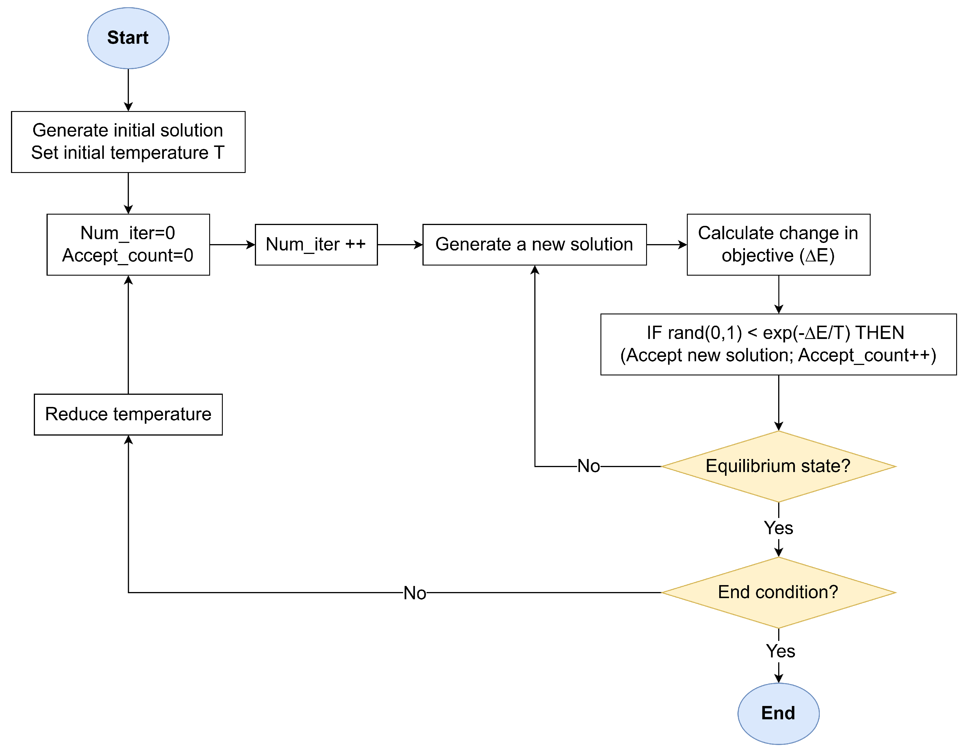
The SA workflow, illustrated in Figure 1, operates through an iterative process that balances stochastic exploration and gradient-driven exploitation. The algorithm begins with a randomly generated or heuristic-guided initial solution $S_{\mathrm{current}}$ and a high-temperature parameter T. The temperature governs the system’s thermal energy, dictating the likelihood of accepting energetically unfavorable states. At each iteration, a neighboring solution $S_{\mathrm{new}}$ is created by perturbing $S_{\mathrm{current}}$ through domain-specific transformations (moves). These perturbations enable the algorithm to explore the solution space without deterministic bias. The fitness of $S_{\mathrm{new}}$ is quantified via an objective function E, often analogous to the system’s energy in physical annealing. The energy difference $\Delta E=E\left(S_{\mathrm{new}}\right)-E\left(S_{\mathrm{current}}\right)$ determines whether $S_{\mathrm{new}}$ is accepted:

• If $\Delta E\le 0$ (improved fitness), $S_{\mathrm{new}}$ is unconditionally adopted.
• If $\Delta E>0$, $S_{\mathrm{new}}$ is accepted with probability $e^{-\Delta E/T}$, derived from the Metropolis–Hastings criterion in statistical mechanics following the Maxwell–Boltzmann distribution.

The temperature T is gradually reduced according to a predefined schedule (e.g., geometric $T_{k+1}=\alpha T_k$, where $0<\alpha <1$). This cooling rate balances exploration (high T) and exploitation (low T), ensuring the system asymptotically approaches a stable equilibrium near the global optimum. At a fixed temperature T, the algorithm generates a sequence of neighboring solutions through random perturbations, which ensures the system attains thermal equilibrium—a state where energy fluctuations stabilize statistically, indicating sufficient exploration of the local solution space. Once equilibrium is achieved at temperature T, the cooling schedule reduces T. This staged approach prevents premature convergence by allowing the algorithm to thoroughly explore regions of interest at each temperature level, mirroring the physical process where materials are held at specific temperatures to enable atomic rearrangement. The process halts when T approaches a near-zero threshold or successive iterations yield negligible energy improvements, signaling convergence.

2.4. SA-Driven Hyperparameter Optimization for CNNs

The optimization process begins with an initial solution vector $S_0$, randomly sampled. This configuration explicitly defines critical parameters such as the learning rate, the type of optimizer, the number and size of convolutional filters, dropout rates for regularization, activation functions, and the neuron count in fully connected layers. The proposed algorithm operates directly on the hyperparameter space without requiring auxiliary encoding, eliminating unnecessary abstraction and preserving interpretability.

Neighboring solutions are obtained by randomly selecting one hyperparameter and reassigning it a new value, uniformly sampled from its predefined set. This single-parameter perturbation strategy designed to maintain gradual exploration. The fitness of each configuration is then quantified using an energy function inversely proportional to the model’s training accuracy:

$$E\left(S\right)=1-Accurac{y}_{\mathrm{train}}\left(S\right)$$

where a lower energy value indicates superior generalization performance by virtue of higher training accuracy.

A geometric cooling schedule orchestrates the algorithm’s transition from exploration to exploitation, progressively reducing the temperature T according to $T_{k+1}=\alpha T_k$, where $\alpha$ (typically $0.8\le \alpha \le 0.95$) controls the cooling rate. At each temperature stage, the algorithm iterates until either two moves are accepted or a trial limit is reached, ensuring adequate exploration of the local search neighborhood before cooling. Termination criteria include sustained performance plateaus—defined as three consecutive temperature stages without energy improvement—or the completion of a predefined maximum iteration count, safeguarding against excessive computational expenditure.

2.5. Algorithm Parameters

The proposed SA-driven hyperparameter optimization framework is governed by a carefully curated set of parameters, designed to balance computational feasibility with robust exploration of the CNN architecture space. These parameters, summarized in

Table 1. Algorithm parameters.

Parameter	Values
Learning Rates	$0.0001$ to $0.001$ in increments of $0.0001$
Optimizers	SGD, Adam, RMSProp
Number of Filters	8, 16, 32, 64
Filter Sizes	3, 5, 7
Dropout Rates	$0.1$ to $0.3$ in increments of $0.01$
Activation Functions	ReLU, LeakyReLU, ELU
Number of Neurons (FC)	32, 64, 128
Epochs per Evaluation	5
Final Training Epochs	20
Maximum Iterations	30
Trials per Temperature	Max 10 moves until 2 acceptances
Termination Criteria	3 consecutive stages without improvement
Initial Temperature	0.0144
Cooling Rate	0.9

, were selected based on empirical benchmarks from medical imaging literature and iterative pilot studies to align with the constraints of brain tumor classification tasks.

The baseline CNN architecture (Figure 2) comprises two convolutional layers followed by two fully connected layers, a design chosen to minimize computational overhead while retaining sufficient representational capacity for MRI-based tumor discrimination. Following the convolutional layers, feature maps are downsampled using fixed $2\times 2$ and $4\times 4$ max-pooling operations. These pooling layers were kept constant (not varied in the search), focusing the optimization on more influential parameters like filter counts, kernel sizes, and activation functions. Dropout regularization is applied before the final fully connected layer to mitigate overfitting, a critical consideration given the limited size of clinical datasets. This streamlined structure ensures compatibility with SA’s iterative evaluation process, where each candidate configuration is initially trained for 5 epochs to quickly assess its fitness, and the best-performing model is then fully trained for 20 epochs for thorough validation.

The hyperparameter search space is constrained to clinically plausible ranges informed by neuroimaging precedents. Learning rates span a narrow interval to stabilize gradient updates, while optimizers are selected to represent distinct gradient descent philosophies—ranging from momentum-driven (SGD) to adaptive learning-rate strategies (Adam, RMSProp). Convolutional filter dimensions and counts are bounded to capture tumor features at varying scales, from localized texture anomalies to broader anatomical context, without exceeding hardware limitations common in clinical settings. Activation functions are restricted to non-linearities proven to balance gradient flow and computational efficiency in medical deep learning, avoiding esoteric choices that might hinder reproducibility.

SA-specific parameters are calibrated to harmonize exploration and exploitation. The initial temperature and cooling rate are tuned to permit early-stage architectural diversity—such as testing aggressive regularization or unconventional filter configurations—while progressively prioritizing refinement as the search converges. Termination criteria and trial limits per temperature stage safeguard against resource exhaustion. These settings ensure the algorithm adapts dynamically to the rugged hyperparameter landscape, where subtle interactions between learning rates, dropout, and optimizer dynamics can disproportionately impact diagnostic accuracy.

Notably, we selected the initial temperature ($T_0=0.0144$) and cooling rate ($\alpha =0.9$) after pilot experiments to balance exploration and efficiency. A higher initial temperature or slower cooling (e.g., $\alpha >0.9$) allowed more extensive search but significantly increased runtime, while lower values led to premature convergence. Empirically, $T_0=0.0144$ ensured balanced acceptance of slightly worse configurations in the first stage (enabling broad exploration), and $\alpha =0.9$ decayed the temperature to near-zero by approximately 20 iterations, focusing refinement thereafter. In summary, these settings reflect a trade-off: enabling sufficient diversity early on without excessive computation, as evident in the convergence behavior of our experiments.

2.6. Dataset

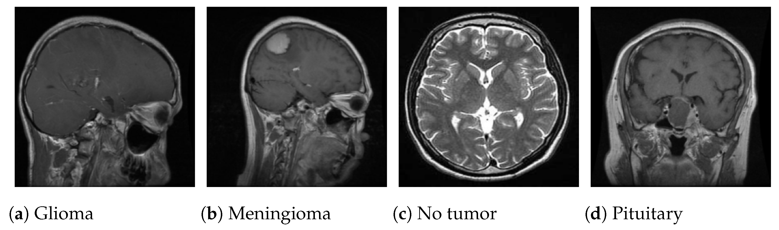
This study leverages a publicly available MRI dataset curated by Nickparvar [35], which consolidates brain tumor scans from three open-access repositories: Figshare, SARTAJ, and Br35H. The composite dataset includes 7023 grayscale axial MRI slices in JPG format, categorized into four diagnostic classes: glioma (1621 images), meningioma (1645 images), pituitary tumor (1757 images), and no tumor (2000 images). Figure 3 displays sample images from each class.

To mitigate class imbalance and preserve distributional integrity, the dataset was partitioned using stratified sampling, allocating 80% of images for training and 20% for validation. Stratification ensures proportional representation of tumor subtypes across both subsets, reducing bias in model evaluation. The resulting splits (

Table 2. Class distribution.

Class	Total Images	Training (80%)	Validation (20%)
Glioma	1621	1297	324
Meningioma	1645	1316	329
Pituitary Tumor	1757	1406	351
No Tumor	2000	1600	400
Total	7023	5619	1404

) provide a balanced foundation for training generalizable classifiers while reserving a clinically representative cohort for validation.

The inclusion of multi-source data introduces heterogeneity in imaging protocols, scanner resolutions, and slice orientations, emulating real-world clinical variability. While the “no tumor” class is marginally overrepresented—a pragmatic concession to enhance specificity in healthy tissue identification—the tumor subtypes maintain near-equitable sample sizes, ensuring the model learns discriminative features across pathologies.

3. Results and Discussion

All experiments were conducted on a Dell notebook equipped with an Intel^® Core™ i7-10510U CPU operating at a base frequency of 1.80 GHz and a maximum turbo frequency of 2.30 GHz. The system featured 8 GB of DDR4 memory. Models were developed in Python 3.8 using the PyTorch 1.10 framework.

The optimization trajectory and performance metrics of the SA-driven hyperparameter tuning process demonstrate significant improvements in diagnostic capability while maintaining computational efficiency. As depicted in Figure 4, training accuracy increased by 2.44 percentage points (92.36% to 94.8%) over 11 iterations, with subsequent stabilization indicating convergence toward a robust configuration. This improvement trajectory reflects SA’s capacity to escape local optima during early high-temperature exploration while progressively refining parameters as the cooling schedule prioritizes exploitation. The final plateau after iteration 11 suggests diminishing returns from further optimization, aligning with the termination criteria of three unchanged stages.

The optimal hyperparameters (

Table 3. Best solution found.

Parameter	Values
Learning Rate	0.0007
Optimizer	Adam
Number of Filters	32, 64
Kernel Sizes	7, 5
Dropout Rates	0.22
Activation Functions	LeakyReLU
Number of Neurons (FC)	128
Number of Parameters	6,479,172

) highlight a balanced architectural design tailored to MRI data characteristics. A learning rate of 0.0007, combined with the Adam optimizer, facilitated stable gradient updates while adapting to intensity variations common across multi-source MRI scans. The use of ascending filter counts (32 to 64) and larger initial kernel sizes ($7\times 7$, $5\times 5$) enhanced the model’s capacity to detect both fine-grained tumor textures and broader anatomical context. LeakyReLU activations mitigated gradient saturation in deeper layers, while a dropout rate of 0.22 provided sufficient regularization to prevent overfitting without suppressing critical tumor signatures. These design choices collectively contributed to the model’s narrow training-validation accuracy gap (99.04% vs. 98.15%), as depicted in Figure 5, indicating strong generalization despite dataset heterogeneity.

Training dynamics further validate the model’s robustness. The training loss decreased exponentially from 0.668 to 0.0283 over 20 epochs, closely mirrored by the validation loss trajectory, which settled at 0.0959 without signs of divergence (Figure 6). This synchronized reduction underscores the model’s ability to generalize rather than merely memorize training data, a critical achievement given the limited size and variability of clinical MRI datasets. Minor validation loss fluctuations, such as the transient increase at epoch 14 (0.254), likely stem from inherent challenges in medical imaging, including scanner-specific artifacts and variations in tumor presentation across patients.

During the SA search, only the training accuracy after 5 epochs was used to evaluate candidate configurations, since this allowed faster fitness assessments. This practical choice can bias the search toward models that perform well on the training set, raising overfitting concerns. Indeed, the final model shows a slight accuracy gap (99.04% train vs. 98.15% validation). The inclusion of dropout (0.22) in the architecture was crucial for controlling overfitting: preliminary trials showed lower dropout allowed higher training accuracy but larger validation gaps, whereas substantially higher dropout hindered convergence. We did not employ early stopping during the search to keep each evaluation consistent. The learning curves (Figure 5 and Figure 6) show that performance plateaued by about epoch 18, suggesting that halting at 20 epochs captured convergence without excessive overtraining.

In addition to filter and dropout tuning, the choice of optimizer was subject to SA optimization. We included SGD, Adam, and RMSProp in the search, training each candidate for the same 5-epoch budget. This uniform epoch count kept comparisons fair but inherently favors faster-converging methods. Under our conditions, Adam consistently achieved higher early accuracy than SGD or RMSProp, leading to its selection in the best configuration. This reflects SA’s tendency to favor configurations that quickly improve under the fixed budget, a practical trade-off for search efficiency. In principle, allowing variable training durations or adaptive schedules could let slower optimizers catch up, but this was beyond our fixed-budget framework.

From a computational perspective, SA introduces nontrivial overhead. Each iteration involves training the CNN for 5 epochs; our full search (14 iterations) took on the order of 854 min (≃14 h) on our hardware. The final CNN contains 6,479,172 parameters (≃25 MB memory). The ultimate 20-epoch training run took about 13.3 min. Thus, while SA significantly increases hyperparameter search time, it yielded a relatively compact, high- performing model. The SA-based HPO demands more computation than a single training run but delivers a model with strong accuracy and moderate size, potentially suitable for resource-constrained deployments.

Over 14 iterations, SA explored variations of learning rate, filter counts, kernel sizes, dropout, and activation. We observe that the model started with 3.22 M parameters (12.28 MB size, 7.43 min training time) and ended with ≃6.45 M parameters (24.59 MB, ≃13.3 min). The trajectory of key hyperparameters and the effect on accuracy were as follows:

• Learning rate: Adjusted between 0.0007 and 0.001. A slight increase from 0.0007 to 0.0009 coincided with an accuracy gain (93.09% to 93.73%), while later reducing the learning rate (Iteration 7 to 8) caused a small drop (93.36% to 93.06%). Overall, learning-rate changes had a moderate effect.
• Filter counts: The first convolutional filters were reduced from 16 followed by 32 to 8 followed by 16 at iteration 3, which increased accuracy from 93.09% to 93.73%. Later increasing filters to 32 followed by 64 at iteration 9 did not improve accuracy (it slightly dropped to 92.95%), likely due to over-parameterization or training difficulties.
• Kernel sizes: The first-kernels size were increased from $3\times 3$ followed by a $3\times 3$ to $5\times 5$ followed by a $5\times 5$ at iteration 2 (accuracy rose to 93.09%) and then to $7\times 7$ followed by a $7\times 7$ at iteration 8 (accuracy dipped to 93.06%), suggesting larger kernels up to a point were beneficial, but excessively large kernels or mismatched kernel changes (e.g., reducing the second-kernels width to $3\times 3$ followed by a $3\times 3$ at iteration 11) had mixed effects. Indeed, at iteration 11 switching the kernels from $7\times 7$ followed by a $7\times 7$ to $7\times 7$ followed by a $3\times 3$ improved accuracy to 94.80%.
• Dropout rate: Changes in dropout (0.14–0.22) had visible impact. Lowering dropout from 0.18 to 0.14 (Iteration 3 to 4) hurt accuracy (down to 92.49%), whereas raising dropout back up (Iteration 4 to 5) recovered accuracy (to 93.36%). Overall, too little dropout appeared to cause overfitting.
• Activation: Switching from ReLU to LeakyReLU at iteration 10 yielded the single largest accuracy jump (from 92.95% to 94.39%). Indeed, activation choice had the strongest correlation with accuracy (corr ≈ 0.92).
• Dense Units: below 64 cause severe accuracy drops, but 128 balances performance and complexity.

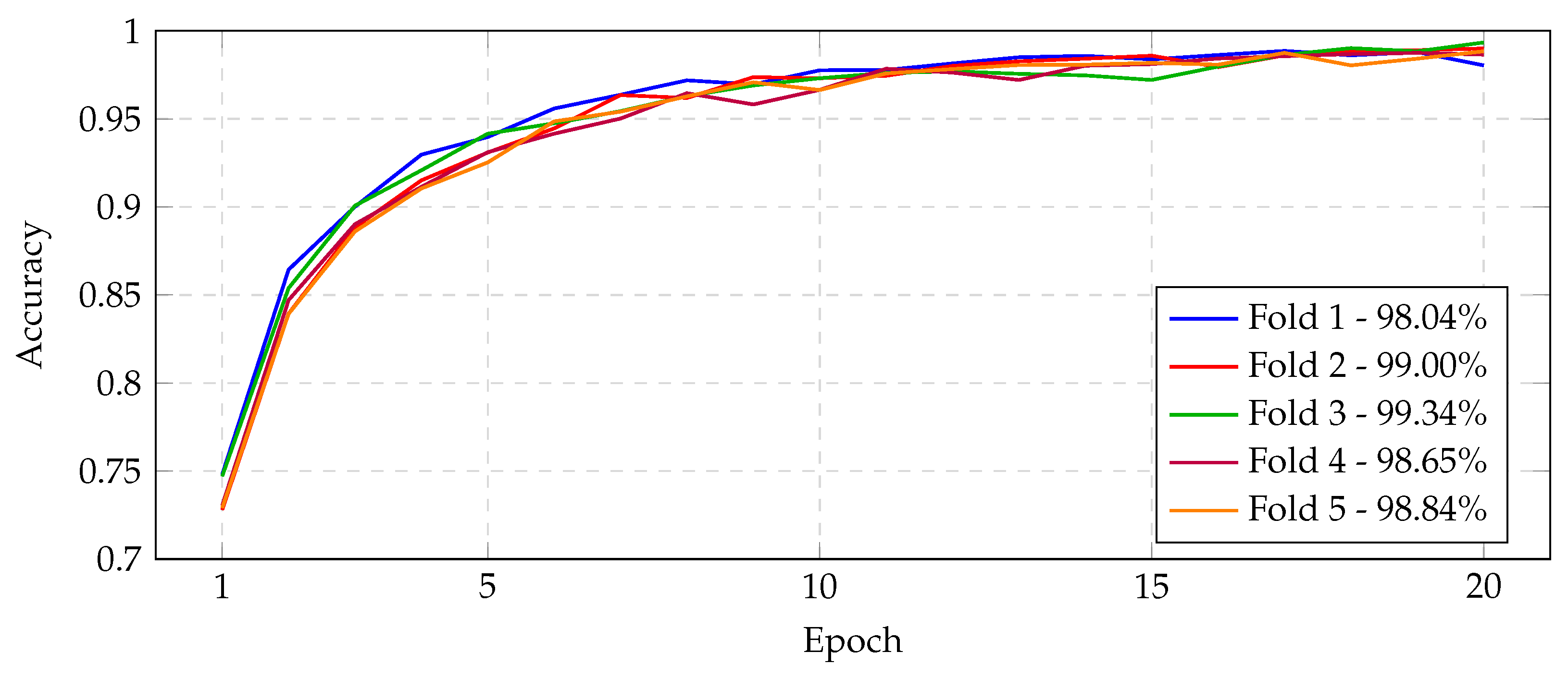
The best CNN model was evaluated under stratified five-fold cross-validation. Overall, the model achieved consistently high validation performance across all folds. Figure 7 (confusion matrices), Figure 8, Figure 9, Figure 10 and Figure 11 (learning and validation curves) illustrate the fold-by-fold outcomes. On average, the model attained a validation accuracy of ≈96.30%, with correspondingly high precision, recall, and F1-scores. Precision and recall were particularly stable: the mean precision was ≈96.28% and mean recall ≈96.17%, indicating a balanced sensitivity and specificity across folds. The Matthews correlation coefficient (MCC) and Cohen’s kappa ($\kappa$) also remained uniformly high (mean ≈ 0.9507 and ≈0.9505, respectively), reflecting strong agreement between predictions and true labels beyond chance.

Examining each fold in detail, fold-level validation metrics were as follows. Fold 1 yielded the lowest accuracy (94.16%) among all folds and high loss (0.1861). Its precision, recall, and F1-score were 0.9415, 0.9397, and 0.9402, respectively, with MCC = 0.9222 and $\kappa$ = 0.9220. In contrast, folds 2 and 4 exhibited the best performance, each achieving validation accuracy 97.44% and low validation loss (≈0.1443 and 0.1491). For these folds, precision was ≈0.9730–0.9745, recall ≈ 0.9733, and F1 ≈ 0.9732–0.9738; MCC ≈ 0.9658 and $\kappa$≈ 0.9658–0.9657. Fold 3 attained intermediate results: accuracy 96.30% (loss 0.2053), with precision 0.9628, recall 0.9614, F1 0.9618, MCC 0.9507, and $\kappa$ = 0.9505. Fold 5 also performed well overall: accuracy 96.15% (loss 0.2977), precision 0.9621, recall 0.9609, F1 0.9607, MCC 0.9491, and $\kappa$ = 0.9486. In summary, across the folds the accuracy ranged from 94.16% to 97.44%, and precision/recall each ranged roughly 93.97–97.45%. The narrow spreads and small standard deviations indicate very consistent performance: in particular, precision and recall closely matched in every fold, showing the model did not favor false positives or negatives.

Average metrics (

Table 4. Summary of the five-fold cross-validation performance metrics for the best CNN model.

Fold	Validation Loss	Accuracy (%)	Precision (%)	Recall (%)	F1 Score (%)	MCC	$\mathit{\kappa }$
1	0.1861	94.16	94.15	93.97	94.02	0.9222	0.9220
2	0.1443	97.44	97.30	97.33	97.32	0.9658	0.9658
3	0.2053	96.30	96.28	96.14	96.18	0.9507	0.9505
4	0.1491	97.44	97.45	97.33	97.38	0.9658	0.9657
5	0.2977	96.15	96.21	96.09	96.07	0.9491	0.9486
Average	0.1965	96.30	96.28	96.17	96.19	0.9507	0.9505
Std. Dev.	0.0620	1.34	1.31	1.37	1.36	0.0180	0.0180

MCC = Matthews Correlation Coefficient; $\kappa$ = Cohen’s kappa coefficient.

) further confirm generalizability. The mean validation loss over all folds was ≈0.1965, mean accuracy ≈ 96.30%, mean precision ≈ 96.28%, recall ≈ 96.17%, and F1 ≈ 96.19%. Mean MCC and Cohen’s $\kappa$ were ≈0.9507 and ≈0.9505. These averages indicate that the model’s performance is robust and consistent across different data splits, supporting its generalizability.

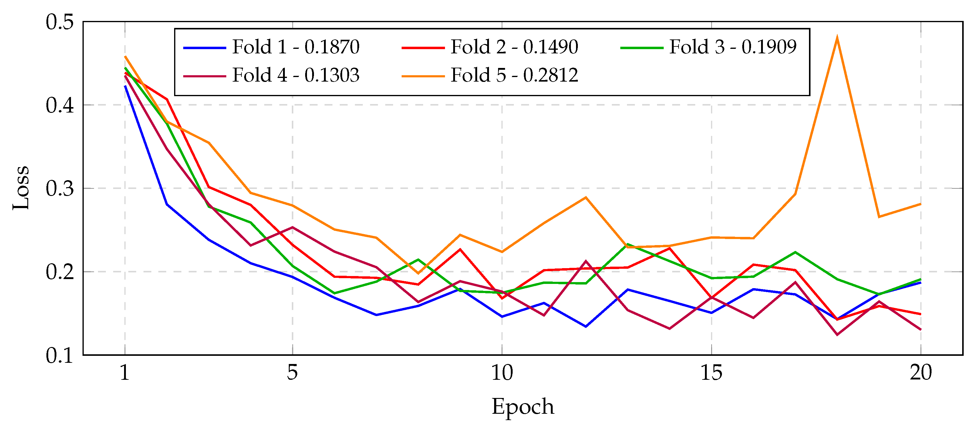
Any anomalies or dips in performance were minor. Notably, fold 1 exhibited the lowest metrics, suggesting that its particular data split may have been slightly more challenging (as also reflected by its confusion matrix in Figure 7). Fold 5 showed the highest validation loss (0.2977) despite still maintaining high accuracy; this may indicate a few harder-to-classify samples in that fold, but the validation curve in Figure 9 shows that the model nonetheless converged smoothly. Importantly, none of the folds showed overfitting or divergent training: all learning curves smoothly decreased loss and increased accuracy on both training and validation sets (see Figure 8, Figure 9, Figure 10 and Figure 11). Overall, the fold-to-fold variability was small and the model’s precision and recall remained stable, confirming that the CNN yields reliable, high-quality classification in this task.

To contextualize our results,

Table 5. Validation accuracy comparison.

Reference	Method	Dataset	Classes	Accuracy (%)
Ref. [17]	Genetic Algorithm-Enhanced CNNs	Figshare [36]	3	94.2
Ref. [18]	Particle Swarm-Optimized CNNs (I)	Combination [35]	4	96.64
Ref. [19]	Particle Swarm-Optimized CNNs (II)	Combination [35]	4	96.8
Ref. [20]	Advanced CNN-Integrated ML Framework	Combination [35]	4	97.93
Ref. [22]	Transfer Learning-Integrated CNNs	Combination [35]	4	97.12
Ref. [23]	Bayesian Optimization-Enhanced CNNs	Figshare [36]	3	98.70
This work	Proposed Framework	Combination [35]	4	98.15

compares the validation accuracy of our approach to selected recent studies. Importantly, these results derive from studies using similar but not identical protocols. While most referenced methods used the same four-class MRI dataset, differences in preprocessing, augmentation, or train-test splits can affect outcomes. As a result, Table 5 provides a broad comparison; nonetheless, our 98.15% accuracy remains competitive with State-of-the-Art under these common conditions.

Notably, the framework outperforms genetic algorithm-enhanced CNNs (94.2%) and both variants of particle swarm-optimized CNNs (96.64%, 96.8%), demonstrating SA’s superior ability to navigate non-convex hyperparameter landscapes without premature convergence. The 1.22 percentage point advantage over advanced CNN–ML hybrids (97.93%) further emphasizes the benefits of holistic architectural tuning via SA, which simultaneously optimizes activation functions, regularization, and feature extraction parameters rather than isolating individual components. While transfer learning approaches (97.12%) reduce training costs through pre-trained feature extractors, their reliance on generic ImageNet-derived representations limits adaptability to MRI-specific tumor morphology, a gap addressed by SA’s direct optimization of domain-tailored architectures.

The proximity to Bayesian-optimized CNNs (98.70% accuracy across three tumor classes) is particularly instructive. They base their design on VGG-16, reducing it to five convolutional layers and two dense layers, and inserting a dropout layer to prevent overfitting—all while preserving the original max-pooling scheme. They apply Bayesian Optimization, which builds a lightweight surrogate model and uses an expected improvement acquisition function to efficiently probe the most promising hyperparameter settings [23]. In contrast, our SA-configured network was deliberately streamlined for a four-class classification task, reducing both model depth and the breadth of hyperparameter exploration to curtail training time and accommodate limited computational resources. Although this leaner architecture and more moderate search space yield a slightly lower overall accuracy of 98.15%, they reflect a practical trade-off between performance and the real-world limitations of hardware capacity and turnaround requirements.

The 98.15% accuracy exceeds the 95% minimum accuracy threshold recommended for auxiliary diagnostic tools in radiological workflows. When contextualized against the Kaggle dataset’s inherent heterogeneity—spanning multiple MRI scanners, slice orientations, and tumor stages—the framework’s generalizability suggests strong potential for real-world adoption, particularly in resource-constrained settings where balancing accuracy and computational costs is paramount.

4. Conclusions

The integration of Simulated Annealing (SA) into hyperparameter optimization for MRI-based brain tumor classification underscores its efficacy in navigating the intricate, high-dimensional search spaces inherent to convolutional neural networks (CNNs). By leveraging SA’s thermodynamic-inspired exploration–exploitation duality, the framework identified configurations that achieved competitive validation accuracy (98.15%), closely approaching the performance of Bayesian-optimized models (98.70%) while significantly outperforming genetic algorithm (94.2%) and particle swarm optimization (96.8%) counterparts. This success stems from SA’s ability to probabilistically escape local optima during early high-temperature phases, coupled with systematic refinement as the cooling schedule prioritizes exploitation.

Despite these strengths, the methodology imposes substantial computational overhead, necessitating iterative model evaluations across temperature stages. While SA’s single-solution focus reduces memory demands compared to population-based approaches, the requirement for multiple truncated training cycles and final full trainings remains resource-intensive, particularly for deeper architectures or volumetric MRI datasets. This trade-off between accuracy and efficiency highlights a central challenge in clinical deep learning, where diagnostic precision must be reconciled with real-world computational constraints.

Future research should address two key limitations: the fixed two-convolutional-layer architecture, and the manual calibration of cooling schedules, which limits automation potential. Hybrid strategies integrating SA with surrogate models or meta-learning could accelerate convergence, while adaptive cooling policies—dynamically adjusting temperature decay based on validation loss trends—might enhance scalability across diverse imaging modalities. By bridging these gaps, SA-driven optimization can evolve into a versatile tool for precision medicine, balancing computational pragmatism with the escalating complexity of modern neuroimaging diagnostics.