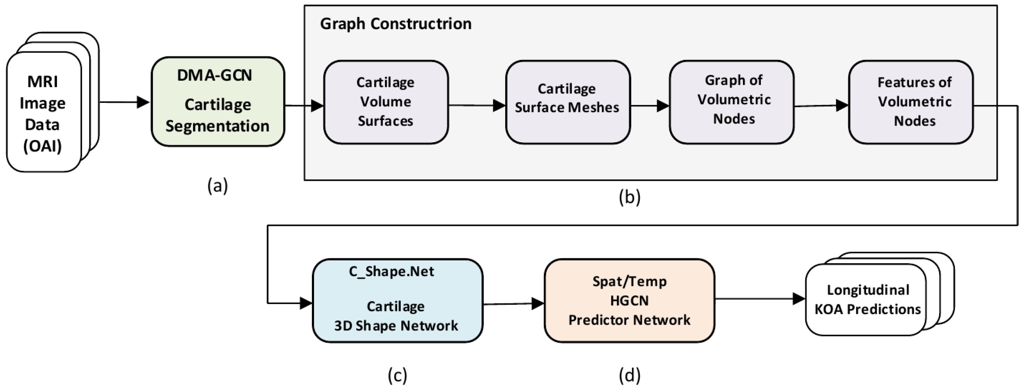
Figure 1.
Overview of the proposed methodology. (a) Preliminary stage of 3D cartilage segmentation. (b) Graph construction of volumetric nodes. (c) C_Shape.Net providing 3D shape descriptors of the cartilage volume. (d) The ST_HGCN predictor network providing longitudinal predictions of KOA grades and progression.
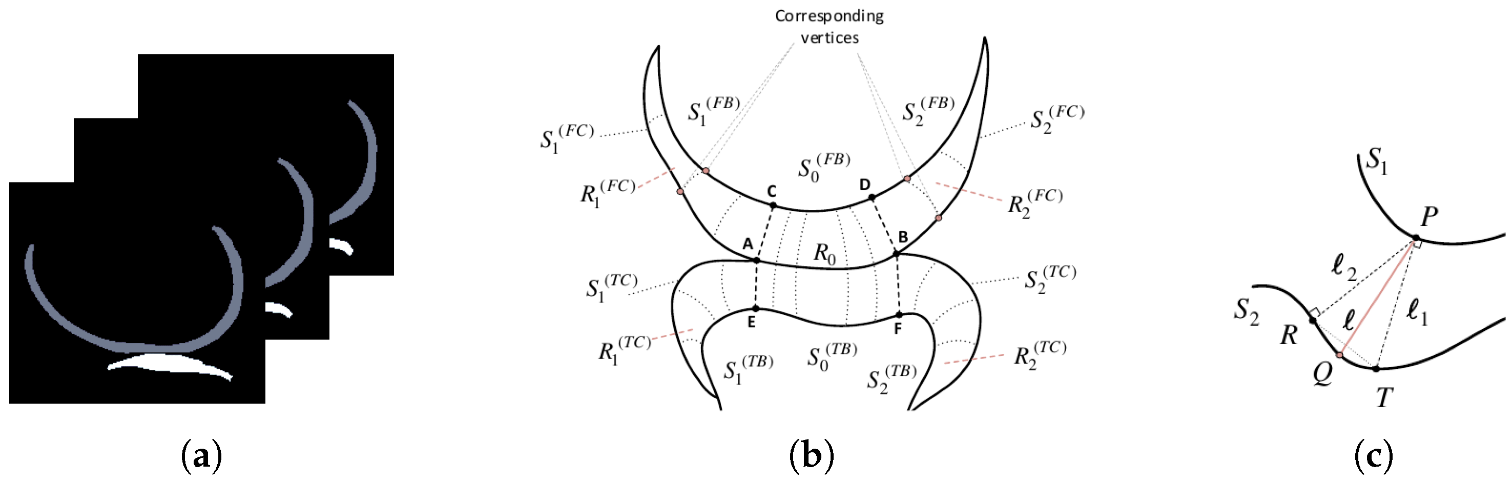
Figure 2.
(a) Slices of an MRI segmentation map, showcasing the femoral (gray) and tibial (white) cartilages in the sagittal plane. (b) A 2D illustrative drawing of a particular slice showing the cartilage regions and surfaces involved. (c) Explanatory scheme describing the formation of corresponding vertices between two surfaces.
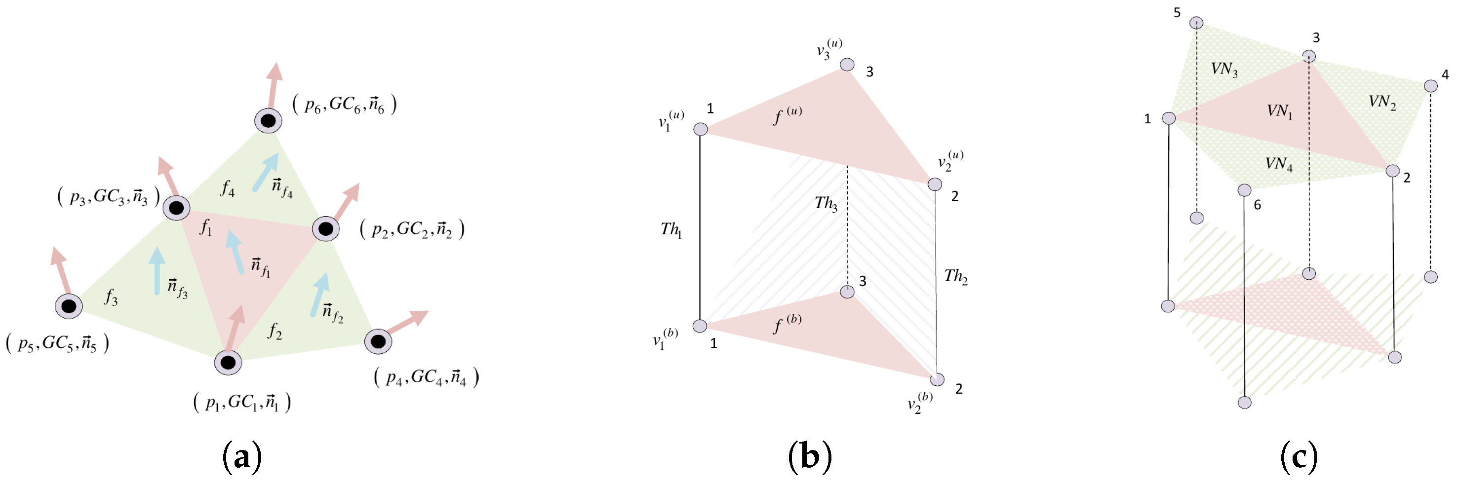
Figure 3.
Cartilage mesh face structure. (a) A 1-ring neighborhood of mesh face. (b) A 3D prism formed by an upper and bottom triangular cell (face). (c) Neighborhood structure around a triangular cell.
Figure 3.
Cartilage mesh face structure. (a) A 1-ring neighborhood of mesh face. (b) A 3D prism formed by an upper and bottom triangular cell (face). (c) Neighborhood structure around a triangular cell.
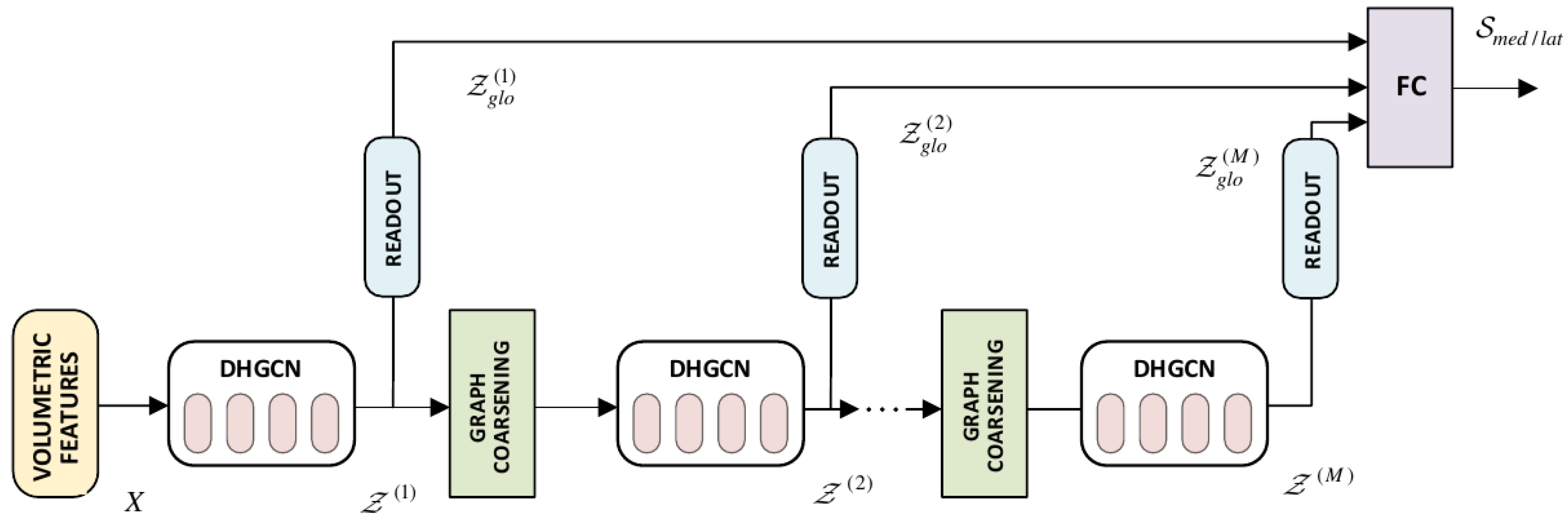
Figure 4.
Proposed C_Shape.Net Hierarchical Architecture. It includes the DHGCN convolutional blocks, the graph coarsening, and readout layers. Global features across the different layers are passed through FC, to provide the global descriptor of a cartilage compartment.
Figure 4.
Proposed C_Shape.Net Hierarchical Architecture. It includes the DHGCN convolutional blocks, the graph coarsening, and readout layers. Global features across the different layers are passed through FC, to provide the global descriptor of a cartilage compartment.
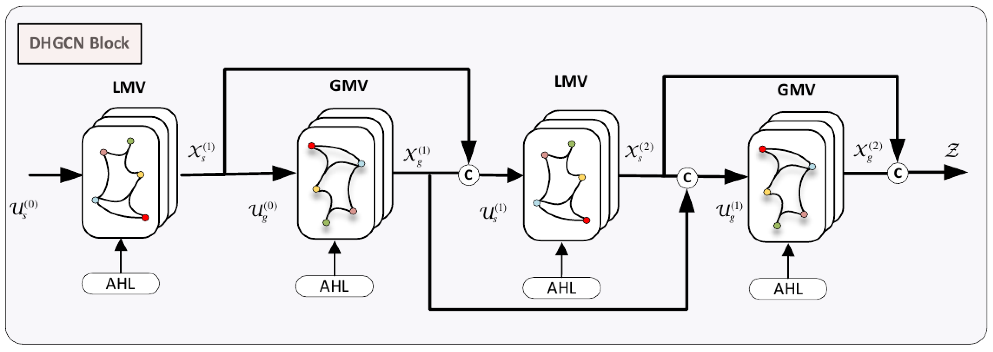
Figure 5.
DHGCN Convolutional Block. It comprises the local multi-view convolutional (LMV) and the global multi-view convolutional (GMV) modules, intertwined into a four-layered model.
Figure 5.
DHGCN Convolutional Block. It comprises the local multi-view convolutional (LMV) and the global multi-view convolutional (GMV) modules, intertwined into a four-layered model.
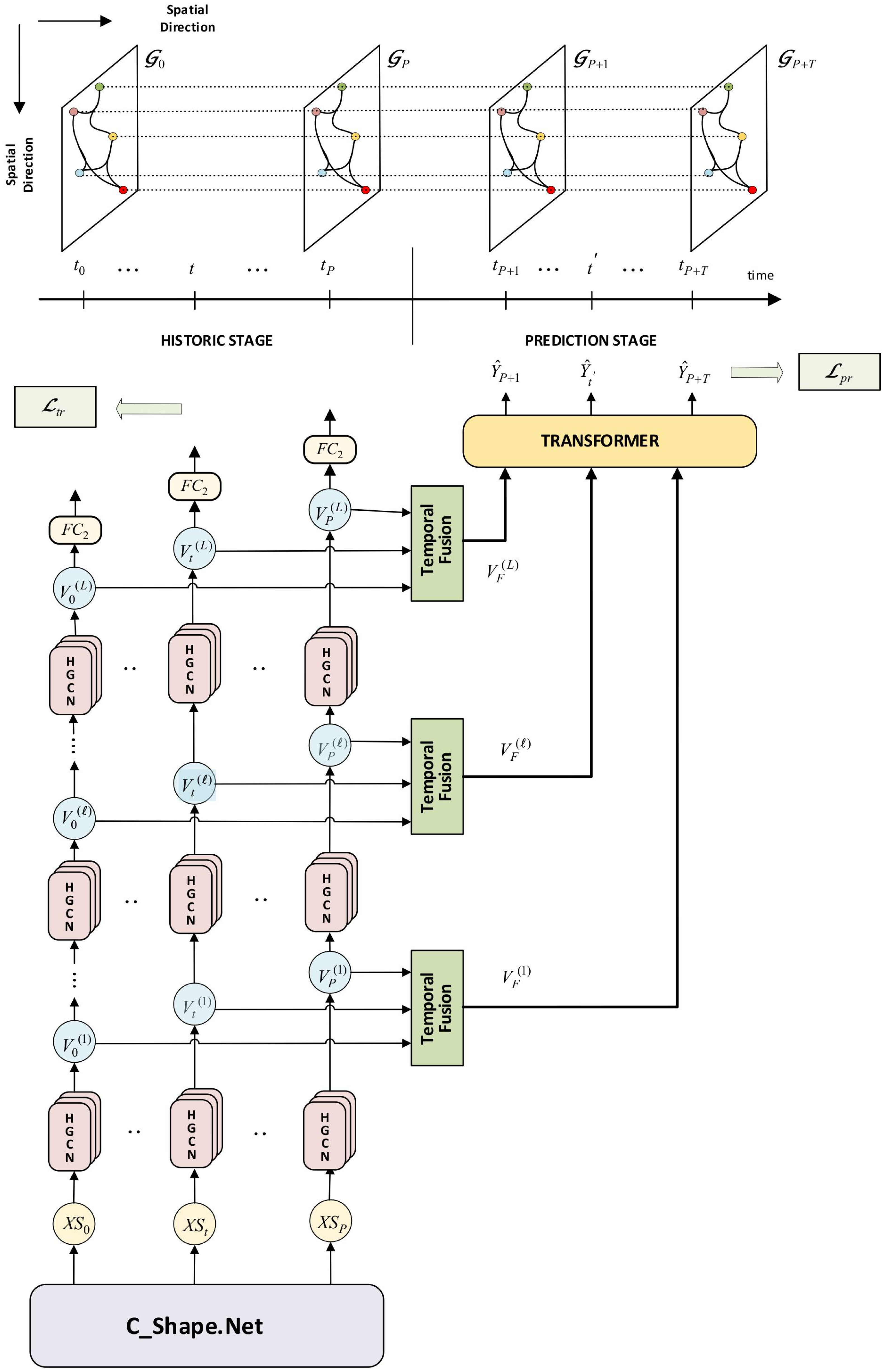
Figure 6.
Proposed ST_HGCN Predictor Network for longitudinal KOA predictions. It incorporates the spatial HGCN convolutions, the attention-based temporal fusion, and the transformer module. Data are distinguished into a historical stage of knee shape sequences, and a prediction stage of KOA prediction sequences. We also show the spatio-temporal interconnection of hypergraphs along the historic/prediction follow-up times.
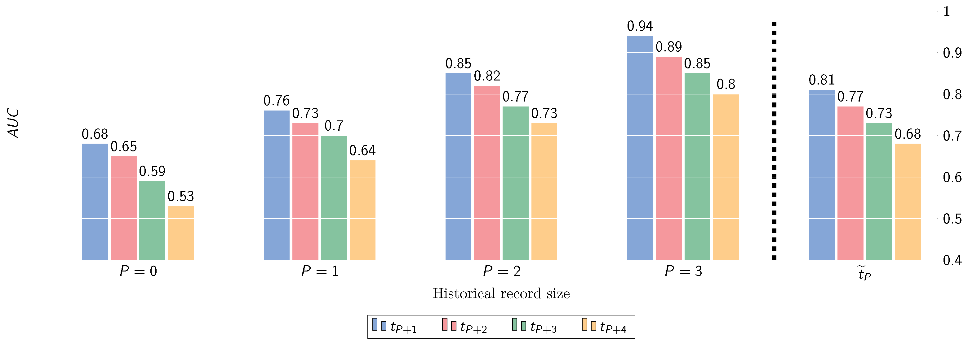
Figure 7.
Performance (AUC) w.r.t. prediction of KOA severity progression (maximum historical depth ), under different transition scenarios. denotes the averaged performance along future time steps.
Figure 7.
Performance (AUC) w.r.t. prediction of KOA severity progression (maximum historical depth ), under different transition scenarios. denotes the averaged performance along future time steps.
Figure 8.
Performance (AUC) w.r.t. prediction of OA progression incidence (KL-grade change ) at multiple time points ahead, for varying historic depths P.
Figure 8.
Performance (AUC) w.r.t. prediction of OA progression incidence (KL-grade change ) at multiple time points ahead, for varying historic depths P.
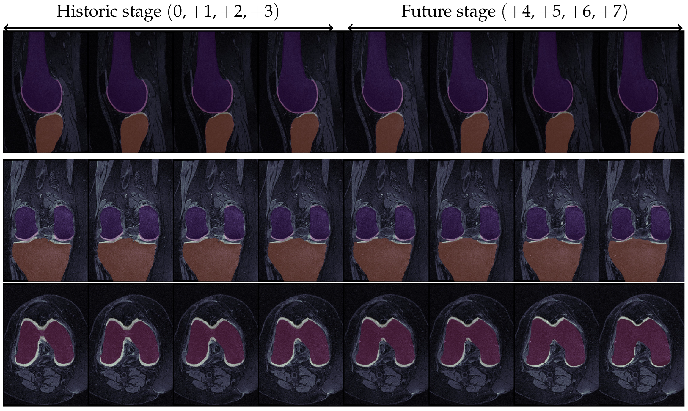
Figure 9.
KOA progression for a specific knee in the OAI dataset. The first four images in each row correspond to the historic stage, while the latter four refer to the prediction stage. For the first two rows, dark orange and dark purple represent the tibial and femoral bones, respectively, while light yellow and light pink represent the corresponding cartilage structures. In the last row, the red part constitutes the femoral bone while the light yellow represents the femoral cartilage. Ground Truth KL-grade progression: / Predicted KL-grade progression: 0 → 0 → 1 → 2 → 2 → 2 → 3 → 4 (green indicates correct prediction, red indicates erroneous prediction).
Table 1.
KL-grade distribution at the multiple historical time points considered in this study.
Table 1.
KL-grade distribution at the multiple historical time points considered in this study.
| | Baseline | 12-Month | 24-Month | 36-Month |
|---|
| 2500 | 2401 | 2369 | 2336 |
| 1206 | 1153 | 1131 | 1082 |
| 1610 | 1645 | 1640 | 1636 |
| 774 | 841 | 863 | 910 |
| 138 | 188 | 225 | 264 |
Table 2.
Summary of the proposed model’s hyperparameter ranges and optimal values determined via Grid-Search + 5-fold Cross-Validation. Bold indicates the optimal parameter value.
Table 2.
Summary of the proposed model’s hyperparameter ranges and optimal values determined via Grid-Search + 5-fold Cross-Validation. Bold indicates the optimal parameter value.
| | #Attention-Heads | Pooling Ratio | Convex Comb. Parameter () | Batch Size | Dropout Prob. |
|---|
| Range & Opt. value | | | | | |
Table 3.
Performance of node KOA classifications under varying-size of historical windows. Results are reported for the Medial/Lateral compartments and their combination. Metrics: [Balanced Accuracy (), F1-weighted measure (), Cohen’s Kappa (K)].
Table 3.
Performance of node KOA classifications under varying-size of historical windows. Results are reported for the Medial/Lateral compartments and their combination. Metrics: [Balanced Accuracy (), F1-weighted measure (), Cohen’s Kappa (K)].
| | Medial | Lateral | Medial + Lateral |
|---|
| P | | | | | | | | | |
|---|
| 0 | | | | | | | | | |
| | | | | | | | |
| 1 | | | | | | | | | |
| | | | | | | | |
| 2 | | | | | | | | | |
| | | | | | | | |
| 3 | | | | | | | | | |
| | | | | | | | |
Table 4.
Performance of KL longitudinal predictions under varying-size of historical windows. Metrics: [Balanced Accuracy (), F1-weighted measure (), Cohen’s Kappa (K), Overall Accuracy averaged across future predictions ()].
Table 4.
Performance of KL longitudinal predictions under varying-size of historical windows. Metrics: [Balanced Accuracy (), F1-weighted measure (), Cohen’s Kappa (K), Overall Accuracy averaged across future predictions ()].
| | | | | | |
|---|
| P | | | | | | | | | | | | | |
|---|
| 0 | | | | | | | | | | | | | |
| | | | | | | | | | | | |
| 1 | | | | | | | | | | | | | |
| | | | | | | | | | | | |
| 2 | | | | | | | | | | | | | |
| | | | | | | | | | | | |
| 3 | | | | | | | | | | | | | |
| | | | | | | | | | | | |
Table 5.
Pairwise comparisons using the Nemenyi statistical test. We evaluate the performance of ST_HGCN under various historical depths for multiple step-ahead predictions. Reported are the corresponding p-values.
Table 5.
Pairwise comparisons using the Nemenyi statistical test. We evaluate the performance of ST_HGCN under various historical depths for multiple step-ahead predictions. Reported are the corresponding p-values.
| | | | | |
|---|
| | | | | | | | | | | | | |
|---|
| | - | - | | - | - | | - | - | | - | - |
| | | - | | | - | | | - | | | - |
| | | | | | | | | | | | |
Table 6.
Balanced accuracy (BA) of KL longitudinal predictions for a historical depth of w.r.t. demographic groups of {Gender, Age, and BMI}.
Table 6.
Balanced accuracy (BA) of KL longitudinal predictions for a historical depth of w.r.t. demographic groups of {Gender, Age, and BMI}.
| | Gender | Age | BMI |
|---|
| | Male | Female | <50 | | | ≥70 | Normal | Pre-Obesity | Obesity |
|---|
| | | | | | | | | |
| | | | | | | | |
| | | | | | | | | |
| | | | | | | | |
| | | | | | | | | |
| | | | | | | | |
| | | | | | | | | |
| | | | | | | | |
Table 7.
Performance of KOA longitudinal predictions for historic depth . Subjects are partitioned according to the stage of KL grades at baseline: : : : . Metrics: [Balanced Accuracy (), F1-weighted measure (), Cohen’s Kappa (K), Overall Accuracy averaged across future predictions ].
Table 7.
Performance of KOA longitudinal predictions for historic depth . Subjects are partitioned according to the stage of KL grades at baseline: : : : . Metrics: [Balanced Accuracy (), F1-weighted measure (), Cohen’s Kappa (K), Overall Accuracy averaged across future predictions ].
| | | | | | |
|---|
| | | | | | | | | | | | | | |
|---|
| | | | | | | | | | | | | |
| | | | | | | | | | | | |
| | | | | | | | | | | | | |
| | | | | | | | | | | | |
| | | | | | | | | | | | | |
| | | | | | | | | | | | |
Table 8.
Prediction accuracies of KOA progression for historical depth . KOA progression of patients over time is categorized according to the following progress classes: Prog+1 indicates the progressions , while Prog+2 indicates the progression . No-Prog refers to subjects that remain static in their respective OA grading. Metrics: [Balanced Accuracy (), F1-weighted measure (), Cohen’s Kappa (K)].
| | | | | |
|---|
| | | | | | | | | | | | | |
|---|
| No-Prog | | | | | | | | | | | | |
| | | | | | | | | | | |
| Prog+1 | | | | | | | | | | | | |
| | | | | | | | | | | |
| Prog+2 | | | | | | | | | | | | |
| | | | | | | | | | | |
Table 9.
Summary of KOA classification results of the proposed method, under varying-size historical windows. We examine the effect of temporal fusion via adaptive attention mechanism vs. temporal fusion via mean aggregation. ATTN indicates temporal fusion via trainable attention mechanism, while MEAN indicates temporal fusion via simple averaging. Metrics: [Balanced Accuracy (), F1-weighted measure (), Cohen’s Kappa (K)].
| | | | | | |
|---|
| | | | | | | | | | | | | |
|---|
| P1 | ATTN | | | | | | | | | | | | |
| | | | | | | | | | | |
| MEAN | | | | | | | | | | | | |
| | | | | | | | | | | |
| P2 | ATTN | | | | | | | | | | | | |
| | | | | | | | | | | |
| MEAN | | | | | | | | | | | | |
| | | | | | | | | | | |
| P3 | ATTN | | | | | | | | | | | | |
| | | | | | | | | | | |
| MEAN | | | | | | | | | | | | |
| | | | | | | | | | | |
Table 10.
Summary of KOA classification results of the proposed method, under varying-size of historical windows. We examine the effect of using solely features learned by ShapeNetvs. incorporating additional demographic data of {Age, BMI, Gender}. Metrics: [Balanced Accuracy (), F1-weighted measure (), Cohen’s Kappa (K)].
| | | | | | |
|---|
| | | | | | | | | | | | | |
|---|
| 0 | ShapeNet + Dem | | | | | | | | | | | | |
| | | | | | | | | | | |
| ShapeNet | | | | | | | | | | | | |
| | | | | | | | | | | |
| 1 | ShapeNet + Dem | | | | | | | | | | | | |
| | | | | | | | | | | |
| ShapeNet | | | | | | | | | | | | |
| | | | | | | | | | | |
| 2 | ShapeNet + Dem | | | | | | | | | | | | |
| | | | | | | | | | | |
| ShapeNet | | | | | | | | | | | | |
| | | | | | | | | | | |
| 3 | ShapeNet + Dem | | | | | | | | | | | | |
| | | | | | | | | | | |
| ShapeNet | | | | | | | | | | | | |
| | | | | | | | | | | |
Table 11.
Summary of KOA classification results under varying-size of historical windows. We examine the effect of using the automatically learned volumetric features extracted by C_Shape.Net vs. computing the Cartilage Damage Index (CDI), at specified points in the MRI scans. Both cases incorporate additional demographic features of {Age, BMI, Gender}. Metrics: [Balanced Accuracy (), F1-weighted measure (), Cohen’s Kappa (K)].
| | | | | | |
|---|
| | | | | | | | | | | | | |
|---|
| 0 | ShapeNet + Dem | | | | | | | | | | | | |
| | | | | | | | | | | |
| CDI + Dem | | | | | | | | | | | | |
| | | | | | | | | | | |
| 1 | ShapeNet + Dem | | | | | | | | | | | | |
| | | | | | | | | | | |
| CDI + Dem | | | | | | | | | | | | |
| | | | | | | | | | | |
| 2 | ShapeNet + Dem | | | | | | | | | | | | |
| | | | | | | | | | | |
| CDI + Dem | | | | | | | | | | | | |
| | | | | | | | | | | |
| 3 | ShapeNet + Dem | | | | | | | | | | | | |
| | | | | | | | | | | |
| CDI + Dem | | | | | | | | | | | | |
| | | | | | | | | | | |
Table 12.
Table showcasing future KL predictions under varying historical depths, against the ground truth values (Predicted Value/Ground Truth).
Table 12.
Table showcasing future KL predictions under varying historical depths, against the ground truth values (Predicted Value/Ground Truth).
| | | | | | | | | |
|---|
| ✗ | | | | | ✗ | ✗ | ✗ |
| ✗ | ✗ | | | | | ✗ | ✗ |
| ✗ | ✗ | ✗ | | | | | ✗ |
| ✗ | ✗ | ✗ | ✗ | | | | |
Table 13.
Comparative performance of KOA prediction methods dealing w.r.t. (1) static KL-grade classification and (2) longitudinal KL-grade prediction and (3) KL-grade progression.
Table 13.
Comparative performance of KOA prediction methods dealing w.r.t. (1) static KL-grade classification and (2) longitudinal KL-grade prediction and (3) KL-grade progression.
| Method | Prediction Type | Data | Source | Add. Inputs | Model | Results |
|---|
| Kishore et.al [29] | KL Grading | OAI | X-ray | - | 12 DL models | |
| Yong et.al [27] | KL Grading | OAI | X-ray | - | {VGG, ResNet, DenseNet} | |
| Gorriz et.al [52] | KL Grading | OAI, MOST | X-ray | - | VGG + Attn. Module | |
| Chen et.al [28] | KL Grading | OAI-baseline | X-ray | - | {ResNet, VGG, DenseNet} + Novel Ord. loss | |
| Zhang et.al [25] | KL Grading | OAI-baseline | X-ray | - | ResNet+ CBAM | |
| Tiulpin et.al [24] | KL Grading | OAItrn.→MOSTtst. | X-ray | - | Deep Siamese CNN | |
| Ashamari et.al [33] | KL Grading | Kaggle | X-ray | - | {Seq.CNN, VGG, ResNet-50} | |
| Proposed | KL Grading | OAI | MRI | - | C_Shape.Net + SptHGCN | |
| Hu et.al [36] | Long. KL Prediction | OAI | X-ray | - | Adversarial NN | |
| Proposed | Long. KL Prediction | OAI | MRI | - | C_Shape.Net + SptHGCN + Transf. | |
| Panfilov et.al. [37] | Long. Progr. Prediction | OAI | X-ray, MRI (multi-modal) | +Demographics | CNN + Transf. | |
| Halilaj et.al. [35] | Long. Progr. Prediction (Progr. vs No-Progr.) | OAI | X-ray | Pain scores (WOMAC) | LASSO + Clustering | |
| Guan et.al. [32] | JSL Progr. (baseline → +48) | OAI | MRI | +{Demographics, Injury hist., Tibiofemoral angle, etc.} | Deep Learning | |
| Du et.al. [34] | KL Progr. Prediction (baseline → +2) | OAI | MRI | CDI at 36 locations | Comparison of ML methods | |
| Ahmad et.al. [33] | Long. Progr. Prediction | OAI | X-ray, MRI (multi-modal) | +Demographics | CNN + Transf. | |
| Tiulpin et.al. [51] | No-Progr. vs Progr. | OAItrn.→MOSTtst. | X-ray | +{Demographics, WOMAC, Injury hist., KL} | DenseNet | |
| Pedoia et.al. [53] | No-OA(≤1) vs OA((>1)) | OAI | MRI | {Demographics, WOMAC} | DenseNet | |
| Alexopoulos et.al. [54] | No_OA vs EARLY_OA | OAI | MRI | +Demographics | {ResNet, DenseNet, CVAE} | |
| Schiratti et.al. [55] | JSN Progr. ahead | OAI | MRI | - | EfficientNet-B0, DenseNet, CVAE | |
| Proposed | KL Progression Incidence | OAI | MRI | +Demographics | C_Shape.Net + ST_HGCN + Transf. | |


