Pattern Matching-Based Denoising for Images with Repeated Sub-Structures

Abstract

In electron microscopy, obtaining low-noise images is often difficult, especially when examining biological samples or delicate materials. Therefore, the suppression of noise is essential for the analysis of such noisy images. State-of-the-art image denoising methods are dominated by supervised Convolution neural network (CNN)-based methods. However, supervised CNNs cannot be used if a noise-free ground truth is unavailable. To address this problem, we propose a method that uses re-occurring patterns in images. Our proposed method does not require noise-free images for the denoising task. Instead, it is based on the idea that averaging images with the same signal having independent noise suppresses the overall noise. In order to evaluate the performance of our method, we compare our results with other state-of-the-art denoising methods that do not require a noise-free image. We show that our method is the best for retaining fine image structures. Additionally, we develop a confidence map for evaluating the denoising quality of the proposed method. Furthermore, we analyze the time complexity of the algorithm to ensure scalability and optimize the algorithm to improve the runtime efficiency.

1. Introduction

Transmission electron microscopy (TEM) imaging is essential in solving numerous scientific questions in life and material sciences [1,2]. However, noise in the acquired images can obscure the signal. This noise can appear due to various reasons like data transmission errors and properties of the imaging systems. In addition, some noise will always be present due to the stochastic nature of the imaging process. Thus, image denoising plays a vital role, especially in high-resolution microscopy.

The contrast in TEM imaging is based on the interaction of a multi-keV electron beam with the specimen. Although the optical resolution for modern TEM system can be below one angstrom, the high-energy electrons required for imaging can lead to a fast degradation of the sample. For sensitive samples, only a few electrons can be used for imaging. This leads to noisy images, thus making the image hard to interpret. Therefore, after image acquisition, numerical processing is essential to enhance the visibility of object structures in the image.

Image denoising has been studied for over 50 years [3], beginning with non-linear, non-adaptive filters [4]. Over time, filtering methods like median filtering [5,6] and bilateral filtering [7] were introduced. A shift from spatial to transform domain methods led to the adoption of wavelet-based techniques [8,9]. Among spatial methods, non-local mean (NLM) [10] emerged as an effective denoising technique. Inspired by NLM, block matching and 3D filtering (BM3D) [11] was introduced, leveraging similarity in image regions for denoising in the transform domain. BM3D remains a widely used classical method, with ongoing improvements [11]. Machine learning methods also play a significant role in denoising. Early approaches [12,13] evolved into deep learning-based methods. CNN-based techniques, such as [14,15], introduced residual learning and improved computational efficiency, demonstrating strong denoising capabilities.

Since, in most cases, very-low-noise electron microscopy images are not available, modern denoising methods that require clean images as ground truths cannot be used. However, there are also some deep neural network-based methods that use noisy supervision [16] and self-supervision [17,18,19]. Although these methods can denoise images, they improve the denoising quality only by a small margin for images with repeated patterns. To solve this problem, a new denoising algorithm which effectively denoises TEM images with repeated patterns is proposed. In our method, we also show that the fine structures in TEM images can be restored most effectively while maintaining image sharpness. In the following sections, the proposed method is explained in detail, and the results are analyzed and compared with state-of-the-art methods, showing significant gains in image quality.

2. Methods

The proposed denoising algorithm identifies similar patches across the entire image and averages them to suppress noise. Mathematically, this approach assumes that the selected patches share the same underlying signal, denoted as s. Each measurement $x_i$ is then modeled as a noisy observation of this signal. Specifically, the measurement follows a Poisson distribution centered around s, potentially influenced by additional noise sources, such as readout noise or random fluctuations. Since the systematic errors in most imaging systems can be compensated, we assume that the noise component has a zero mean. Consequently, the ith measurement can be expressed as

$$x_i=s_i+n_i$$

(1)

Averaging over k patches results in an expected value, as follows:

$$E\left[{\displaystyle \frac{1}{k}}\sum _i^k{x}_i\right]=E\left[{\displaystyle \frac{1}{k}}\sum _i^k(s_i+n_i)\right]$$

(2)

Since we assume the noise component to have a zero mean and since the base signal, s, is expected to be the same, this ideally means that

$$E\left[{\displaystyle \frac{1}{k}}\sum _i^k{x}_i\right]=E\left[{\displaystyle \frac{1}{k}}\sum _i^k{s}_i\right]+E\left[{\displaystyle \frac{1}{k}}\sum _i^k{n}_i\right]=s$$

(3)

However, the variance of the averaged result is

$$Var\left[{\displaystyle \frac{1}{k}}\sum _i^k{x}_i\right]=Var\left[{\displaystyle \frac{1}{k}}\sum _i^k{s}_i\right]+Var\left[{\displaystyle \frac{1}{k}}\sum _i^k{n}_i\right]={\displaystyle \frac{1}{k^2-1}}\sum _i^{k}Var\left[n_i\right]$$

(4)

since $Var\left[s_i\right]=0$ for all i, due to the fact that $s_i$ is a constant and not a random variable. Therefore, its variance is zero. Hence, averaging patches with the same signal suppresses noise.

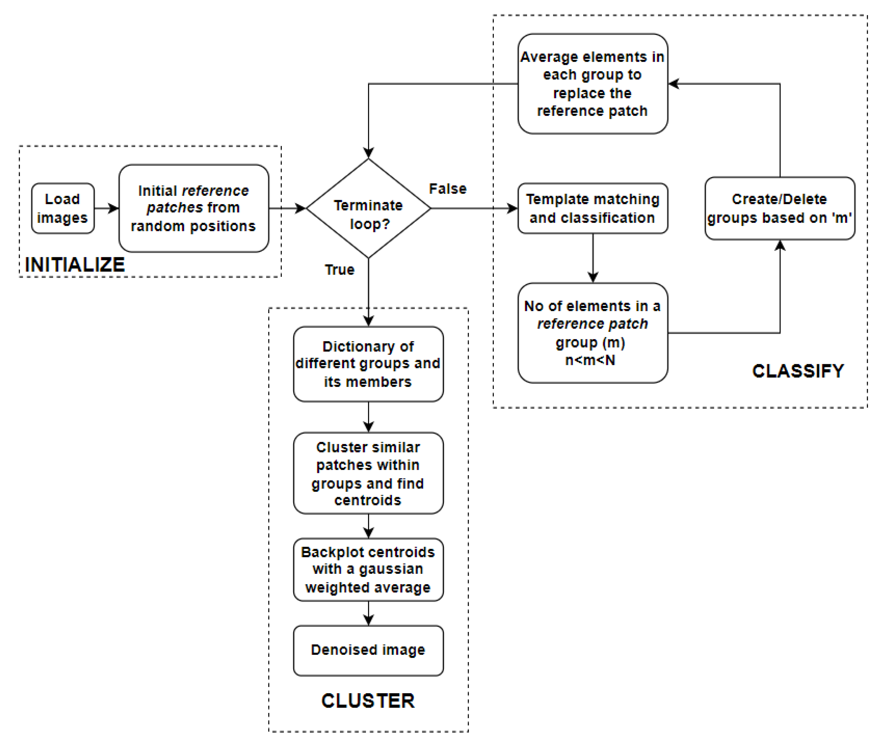
2.1. Outline of the Proposed Algorithm

The proposed algorithm groups similar patches at two levels. Cosine similarity is used to broadly group similar patches within an image. Later, clustering is used to more finely group closely matching patches within the groups obtained during the first step. A flowchart of the algorithm is shown in Figure 1, and the two levels of the algorithm are represented by ‘classify’ and ‘cluster’ sections of the flowchart.

Cosine similarity measures similarities between two vectors [20] by finding the cosine angle between them. If the vectors are in the same direction (i.e., similar), cosine similarity is maximum. It is mathematically represented as

$$sim(A,B)=cos\left(\theta \right)={\displaystyle \frac{A·B}{\parallel A\parallel \parallel B\parallel }}={\displaystyle \frac{{\sum }_{i=1}^n{A}_i{B}_i}{\sqrt{{\sum }_{i=1}^n{A}_i^2}\sqrt{{\sum }_{i=1}^n{B}_i^2}}}$$

(5)

where A and B are two vectors, and $\theta$ is the angle between them. Cosine similarity between a template and different patches of an image results in an array whose values lie between −1 and 1. Values close to the maximum represent the patches similar to the template. Hence, cosine similarity can be used to match two image patches by considering them as vectors.

The algorithm can be divided into three broad sections. Each of the sections is explained below.

2.1.1. Initialize Section

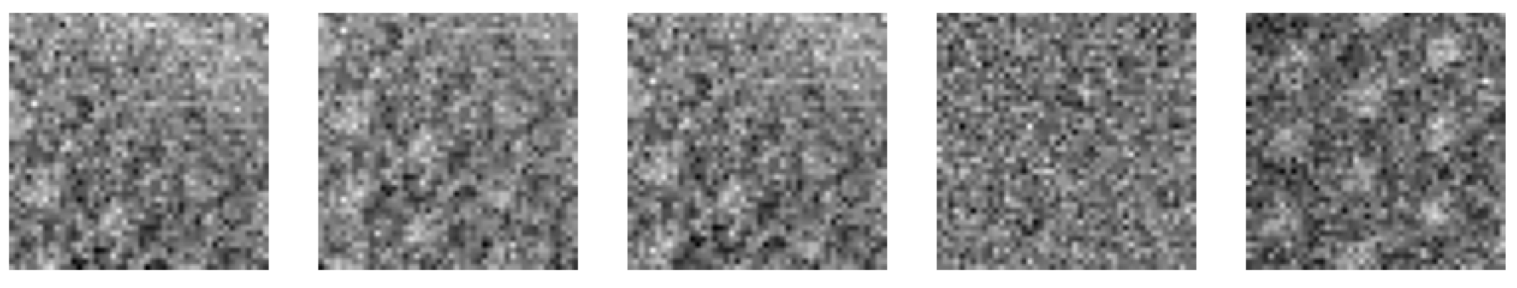
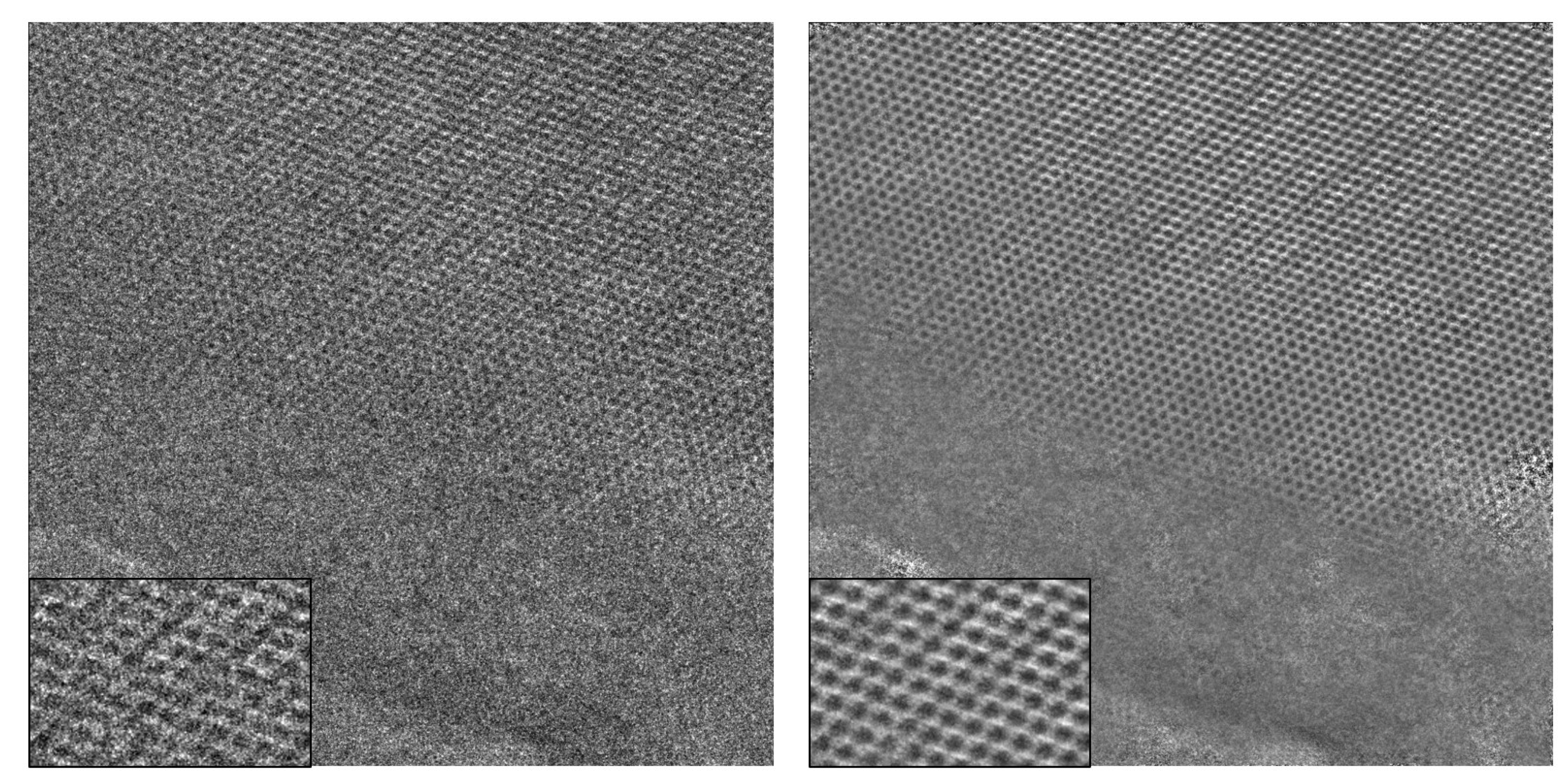
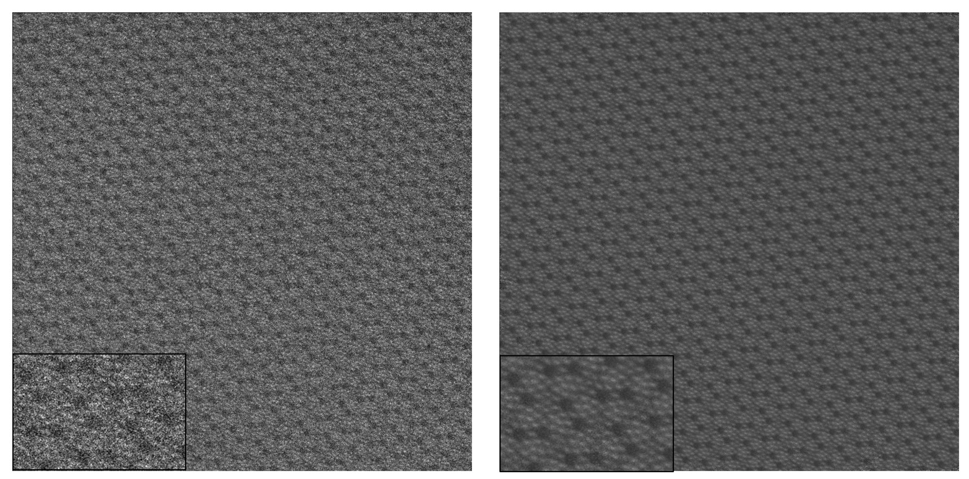
The algorithm begins with the initialization of random patches of size $m\times m$, which are used for matching other patches of the same size in the image. The patches that are used as templates for matching are referred to as reference patches. One example for the initial choice of reference patches can be seen in Figure 2.

2.1.2. Classify Section

In the ‘classify’ section shown in Figure 1, the patches at every position in the image are classified into different groups based on their similarity to the reference patch using cosine similarity. When cosine similarity is applied, each patch of size $m\times m$ in the image is compared with all the reference patches. Local maxima are found from each cosine similarity result, which corresponds to the best-fitting positions for that particular reference patch. These resulting arrays from different reference patches are stacked together and the maximum along the new dimension corresponds to the best-fitting reference patch for different locations of the image. Now that the patches in the image which are most similar to the reference patches are identified, they can be grouped together.

Some of these formed groups can sometimes have a large number of patches in the same group, while others may contain only a few unique patches. Groups with few members contribute little to the denoising, while overly large groups might lead to a loss of detail. Hence, the formed groups are deleted or split into finer groups based on the group size. Finally, for each new group, the old reference patch is replaced by the average of all the members in that group. In the next iteration, cosine similarity and the classification steps repeat with these new reference patches. When the classification becomes stable, there are no new groups formed. This is when the iteration loop is broken. 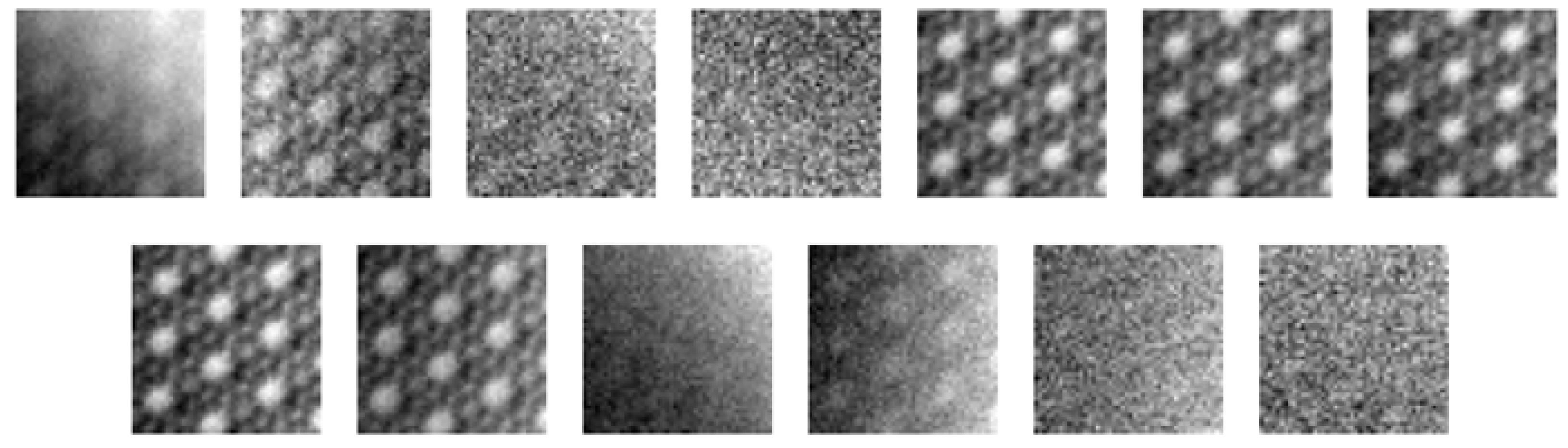Figure 3 shows the reference patches generated after 15 iterations. Upon comparing Figure 2 and Figure 3, one can observe that the noise in the final reference patches is significantly suppressed.

If the final reference patches are directly used for back-plotting (i.e., to replace the patches from their corresponding positions in the image), there would still be some artifacts present. This could sometimes arise because image patches that are not similar to any of the reference patches end up falling into the best available group, even though the group might not be their best representation. This is required since the entire region of the image has to be covered. When outliers are included during averaging, the mean deviates from the median signal value. Additionally, the unique features present as outliers will be lost in the averaging process. Both of these are undesirable. Another reason for artifacts is that cosine similarity is only sensitive to the structure for any two patches and ignores the offset (i.e., brightness). Therefore, back-plotting might not recover local brightness variations.

2.1.3. Cluster Section

The above-mentioned problems can be solved by averaging over a small group with very closely matched patches. To achieve this, clustering is applied within each group (represented by the final reference patch) to create smaller subgroups. The number of clusters in a group can be adjusted using a user-set parameter. In other words, the target signal-to-noise ratio can be adjusted by changing this parameter value. Although the whole group was previously represented by a single reference patch, it is now represented by centroids of the subgroups after clustering. Centroids are back-plotted with a 2D Gaussian-weighted average. These Gaussian weights smooth the edges of the centroids, thus preventing artifacts from appearing in the reconstructed image.

The implementation of the denoising algorithm can be found on GitHub (https://github.com/mbanil/img_denoiser/) (accessed on 18 March 2025).

2.2. Parameters of the Algorithm and Stability

For optimal performance, the algorithm can be fine-tuned using a few user-adjustable parameters. These include the patch size and, if needed, the upper and lower limits of the group size for cosine similarity classification, depending on the desired level of denoising. The initial patch positions can also be specified as an optional parameter. Additionally, the group size for clustering, controlled by the clustering parameter, can be adjusted to enhance the signal-to-noise ratio. If the average number of elements in a subgroup is $N^2$, the signal quality is improved by approximately a factor of N [10].

The patch size should align with the characteristic repetitive features of the image. A smaller patch size increases the number of patches to be compared, significantly affecting computation time. Considering this trade-off, the patch size for the experimental image was set to 48 × 48.

The selection of initial patches influences the convergence speed. The algorithm is most efficient when these patches represent diverse regions of the image, ensuring effective classification. To achieve this, the initial patches are randomly initialized while maintaining adequate spacing. Alternatively, users can manually specify this parameter to better adapt the algorithm to specific requirements.

The clustering parameter regulates the degree of denoising. Although higher values of this parameter can increase noise reduction, they may also diminish sharpness [21]. Therefore, selecting an appropriate value depends on the specific requirements of the task. In our implementation, this parameter is constrained to be greater than 1, with optimal performance observed for values between 2 and 4 in our experiments.

3. Results

The images presented in this paper were captured using electron microscopy in bright-field mode. The pixel values typically range in the order of ${10}^6$. These images are inherently noisy, with shot noise being the primary type of noise present [22,23]. However, since a noise-free reference is unavailable, the exact intensity of the noise cannot be quantified.

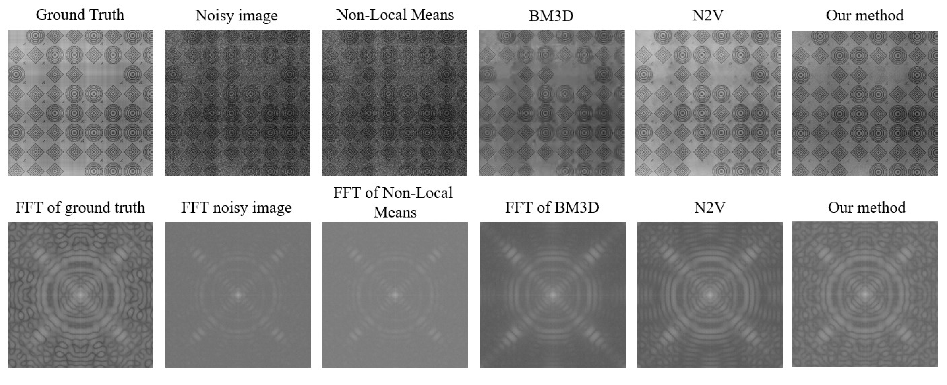
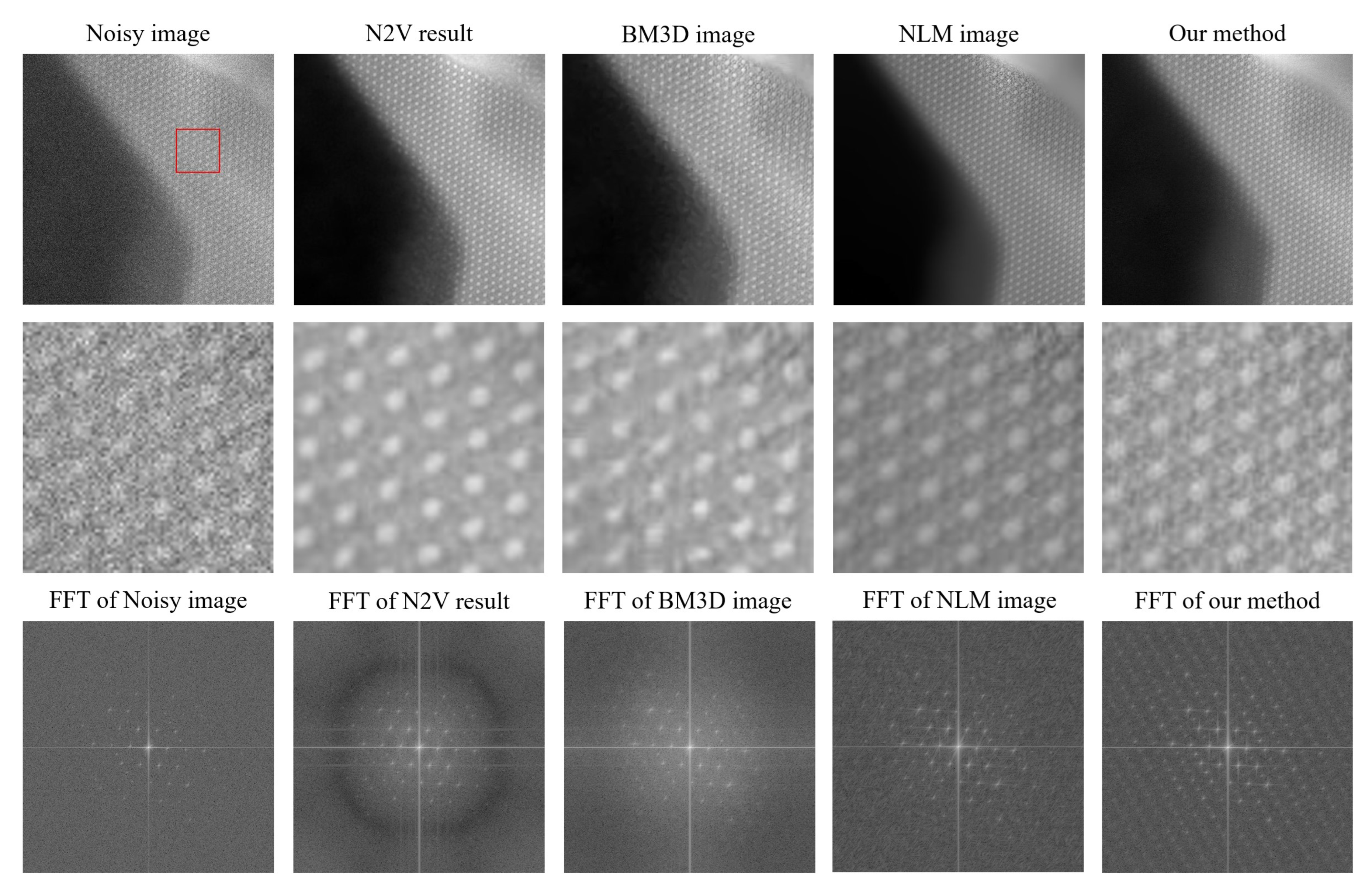
The proposed algorithm is primarily designed to denoise TEM images with repeated structures. However, it can also be applied to other image types and can handle different types of noise. In Figure 4, the results from all the methods and their fast Fourier transforms (FFTs) can be seen for the noisy image. The FFT converts data from the spatial domain to the frequency domain. The signal corresponding to the low-frequency components is represented at the center of the FFT, and higher-frequency components are present as we move away from the center. Noise corresponds to the unstructured background, as seen in the high-frequency region of the FFT, and it is present close to the edges.

When analyzing Figure 4 for the noisy image, we note that it contains numerous grainy structures, which makes it hard to interpret the information. This is also reflected in the FFT, where clear structures are only visible close to the center. In Figure 4, the noisy image is followed by denoised results obtained from different methods.

N2V [17] is a self-supervised, deep learning-based image denoising method. N2V was trained with the patches of the noisy image. The training was carried out with $64\times 64$ patches, 100 epochs and a neighboring radius of 5. The results from N2V show reasonably well-reconstructed circular structures, with the noise in the black region of the image being removed fairly well. However, the sub-structures were not reconstructed accurately. The FFT shows enhanced structures at the center, whereas the boundary mostly looks dark, indicating the suppression of high-frequency noise.

BM3D [11] is one of the most widely used classical denoising methods. BM3D uses collaborative filtering in the transform domain for denoising images. It is a non-blind denoising method, which means that the standard deviation of the noise is required for denoising. The standard deviation was estimated by trial and error. We obtain the best results for a standard deviation of 0.06 for the normalized image. The result from BM3D is similar to that obtained from N2V. The denoising effect is visible but the images are still not very useful for further analysis. This conclusion is also supported by the FFT.

Non-local mean (NLM) denoising [10] is a conventional image denoising method that finds similar patches of images within a region and averages them to suppress noise. An NLM implementation with a patch size of $48\times 48$, a search area of $100\times 100$, and a cut-off distance of 0.36 was used. The result shows a good level of denoising. Circular structures and their subsequent sub-structures are generally more visible, and noise suppression is effective in most regions. However, at some regions, noise is still present. The FFT also shows stronger structures supporting our conclusion of image feature enhancement. Overall, the results look good and more interpretable.

Results of our proposed denoising algorithm were obtained with a patch size of $48\times 48$, a group size between 5 and 100, and a clustering parameter equal to 2.7. From the denoised result, it can be observed that the quality of denoising is marginally better than that from NLM. Noise suppression is the highest compared to the other methods, and information in the image can be interpreted the best from it. The sub-structures between the circular structures are also more visible. From the FFT, we also see that the structures are more prominently visible. Some features can also be seen in the high-frequency region, but were not visible so well previously.

The denoising results of additional experimental images can be found in Appendix B.

Apart from the qualitative improvement in the results, the proposed algorithm has a bigger advantage with regard to the computational time. Most of the computational time is spent in the ‘classify’ section (see Figure 1) of the algorithm, where image patches are matched with reference patches. Initially, this process relied on template matching; however, it has since been improved using cosine similarity, which utilizes convolution operations instead of the traditional template matching approach. The time complexity of the convolution operation is $O\left(m^2{n}^2\right)$, where $m\times m$ is the size of the patch and $n\times n$ is the size of the image, which is worse than the runtime of the template matching algorithm when m is large. Complexity of the template matching algorithm is $O\left(n^{2}log\left(n^2\right)\right)$ [24], where $n\times n$ is the image size. Since the convolution operation is widely used in convolution neural networks, there are Python (http://www.python.org) libraries like Pytorch (https://pytorch.org/) that support GPU computations for performing this operation. Running computations on the GPU makes the algorithm significantly faster.

The proposed method achieved a runtime of 19.4 s for the images in Figure 4, whereas NLM—the closest method in terms of qualitative results—took 171.4 s. This significant reduction in runtime is particularly beneficial for denoising image stacks from transmission electron microscopy (TEM), where consecutive images are often similar. In such cases, our algorithm not only matches templates within the current image but also utilizes patches from other images in the stack, leading to improved denoising quality. With GPU acceleration, the computation speed remains high. For reference, denoising a TEM image stack containing 10 images, each of size 1024 × 1024 pixels, took 281.8 s. In terms of memory usage, the cosine similarity operation is performed on the GPU, while the CPU handles only the patch keys or indices, making the process memory-efficient. The clustering step, performed on the CPU, is also memory-efficient, as it operates within subdivided groups, ensuring that clustering is conducted only within these smaller subsets. These computations were performed on a system equipped with 128 GB of RAM, an Intel Xeon processor (16 CPUs), and an NVIDIA RTX 6000 GPU.

3.1. Comparison with Sample Images

Since obtaining low-noise images is often very difficult in microscopy, we generated a noise-free image (ground truth) artificially for a quantitative comparison. The generated image imitates the kind of microscopy images that are best suited for our algorithm’s application, i.e., images with similar patterns spread across them. Since Poisson noise, also known as shot noise, is the primary type of noise in electron microscopy images [22,23], a noisy image is simulated by adding Poisson noise to the generated image. In the absence of a benchmark method, different denoising methods were applied on this noisy image. Moreover, the peak signal-to-noise ratio (PSNR) and structural similarity index metric (SSIM) values of the denoised images were found with respect to the ground truth. The ground truth, noisy image and the results from different methods can be seen in Figure 5. Additionally, a comparison of the FFT of these images is shown in the Additional Information Section.

The results from non-local mean denoising show minimal improvement. The reason for this is that this method requires similar image patches that are present close to each other, which is not always the case in generated images. BM3D processes the image in the Fourier domain and hence suppresses the high-frequency components. This results in the sharp features of the image being less prominent. N2V presents better denoising capabilities, which is reflected in its PSNR value. However, upon a close inspection, it can be observed that the high-frequency components appear slightly blurred. This is where our method outperforms the others. Our pattern-matching strategy finds similar patterns across the image, thereby ensuring accuracy and also preserving sharpness in the image. This is also reflected by its higher SSIM value. For further comparison, the FFTs of the denoising results are provided in the Appendix A.

It should be noted that PSNR is based on the mean square error and is a distortion-based evaluation metric. In image restoration, there is always a trade-off between the distortion and the perceptual quality of the restored image. Often, it is not possible to achieve both simultaneously [21]. As shown in Figure 5, we obtain the best results with our method for SSIM, which is a more perceptual metric, although we do not achieve the best PSNR value [21].

3.2. Confidence Map

In the absence of a ground truth, it is difficult to identify artifacts in the denoised results. However, it is essential to recognize these artifacts in order to prevent incorrect interpretations of the denoised images. Since detecting minute artifacts from FFTs is challenging, a confidence map is introduced. This map is derived from the variance within each cluster obtained after applying the clustering step, providing a more reliable way to assess artifacts. The idea behind this approach is that the variance should be small if the centroid represents its members well. Also, a good centroid should not have any patterns in its variance. Patterns in the variance indicate that the centroid does not generalize its members well.

To compute the confidence map, the variance of the clusters is calculated during the clustering step. This information, along with the centroids and Gaussian weights used for back-projection to obtain the denoised image, is then utilized to compute weighted variance [25] across different regions of the image. The resulting variance map, also called the confidence map here, is shown in Figure 6. For demonstration purposes, this result was generated using a very limited number of initial reference patches positioned in close proximity to each other, and the ‘classify’ part of the algorithm was interrupted before convergence. The bright regions in the confidence map correspond to the denoised image artifacts. For instance, a bright region can be seen in the confidence map at the top-right position. An artifact can be found by inspecting the same region in the denoised image. Similarly, irregularities in the black region on the left side of the denoised image can be recognized by the brighter regions of the confidence map.

4. Discussion

Denoising of the experimental images obtained from electron microscopy was performed using popular denoising methods—N2V, BM3D, and NLM. Even though these methods successfully suppressed noise, they enhanced fine image features only by a small margin. To address this problem, a new denoising algorithm was developed, which makes use of similar patterns present in images and averages them to suppress noise. This new method successfully denoises images and enhances fine structures. The results of all the denoising methods are compared using FFT. Additionally, a confidence map is developed to evaluate the denoising results when ground-truth data are absent. A quantitative comparison of the denoising results is performed using an artificially generated image. The quantitative comparison demonstrates the ability of our proposed method to preserve high-frequency components in images.

The time complexity of the algorithm was analyzed. Optimizations were made to enhance the computation speed by introducing cosine similarity instead of template matching. This helped in enhancing the runtime efficiency by a significant factor, which ensures scalability.

5. Conclusions

Our proposed method is particularly useful for investigating semi-crystalline materials containing light elements, which are difficult to visualize in TEM images due to low contrast and beam sensitivity. By effectively reducing noise and enhancing contrast, our approach improves the clarity of fine structural details, enabling a better analysis of crystallinity, defects, and amorphous regions. This advancement is especially valuable for material science and polymer research, where nano-scale characterizations are essential.