Optimisation-Based Feature Selection for Regression Neural Networks Towards Explainability

Abstract

Regression is a fundamental task in machine learning, and neural networks have been successfully employed in many applications to identify underlying regression patterns. However, they are often criticised for their lack of interpretability and commonly referred to as black-box models. Feature selection approaches address this challenge by simplifying datasets through the removal of unimportant features, while improving explainability by revealing feature importance. In this work, we leverage mathematical programming to identify the most important features in a trained deep neural network with a ReLU activation function, providing greater insight into its decision-making process. Unlike traditional feature selection methods, our approach adjusts the weights and biases of the trained neural network via a Mixed-Integer Linear Programming (MILP) model to identify the most important features and thereby uncover underlying relationships. The mathematical formulation is reported, which determines the subset of selected features, and clustering is applied to reduce the complexity of the model. Our results illustrate improved performance in the neural network when feature selection is implemented by the proposed approach, as compared to other feature selection approaches. Finally, analysis of feature selection frequency across each dataset reveals feature contribution in model predictions, thereby addressing the black-box nature of the neural network.

1. Introduction

Artificial Intelligence (AI) and machine learning (ML) have significantly enhanced decision-making across various domains. Regression is a key task in machine learning and has been widely studied in the literature [1,2]. Its primary aim is to model the underlying relationship between independent and dependent variables, enabling accurate predictions based on available data samples. Some of the most widely used regression analysis techniques are linear regression, Lasso regression [3], decision trees [4], random forests [5], and support vector regression [6]. Neural networks, a family of powerful learning algorithms, have been successfully applied in numerous applications to model complex relationships between inputs and outputs [7,8,9].

Employing neural networks instead of a simpler, inherently interpretable regression approach may result in accurate predictions [10]; however, their black-box nature results in lack of decision rule tracing. Their underlying model relies on a weight matrix, which is complex and difficult to understand, and their success, driven by multiple layers of non-linear functions, comes at the cost of interpretability [11]. As a result, the absence of justification for neural network predictions can create mistrust in high-stakes domains, and Explainable Artificial Intelligence (XAI) techniques for regression have been employed in many practical application scenarios such as healthcare [12,13,14,15], energy engineering [16], computer vision [17], and criminology [18] to enhance the trustworthiness of predictions. Interpretability and explainability in machine learning arise from this need to develop intelligible machine learning models [19]. Explainable machine learning typically aims to provide post hoc explanations for black-box models to offer insights into their behaviour [20]. In contrast, interpretable machine learning focuses on designing models that inherently allow users to understand their predictions by following a transparent and comprehensible rule that links inputs to outputs [21].

Explainability in neural networks is often linked to simplicity, which can be enhanced by pruning hidden nodes to reduce the complexity of the network, together with pruning the corresponding connections. Moreover, selecting the most important input nodes, known as feature selection, simplifies the network and provides insights into their significance. These complexity reduction techniques can be performed either during training, such as through L1 regularisation, which encourages sparser weight matrices, or post hoc by pruning individual weights with small values or entire neurons that do not significantly affect the model predictions.

Feature selection, in particular, can play an important role in enhancing neural network performance and explainability. By identifying and retaining only the most relevant features, noise and redundant inputs are eliminated from the dataset, making it easier to analyse which factors truly influence predictions. This reduction in input dimensionality can improve model generalisation by reducing overfitting, ensuring that the model learns meaningful patterns rather than capturing noise. Additionally, with fewer features, the relationship between inputs and outputs becomes more transparent, facilitating understanding of the model decision-making process.

Some widely used post hoc explanatory approaches, such as SHAP [22] and LIME [23], explain neural networks by assigning importance to input features based on their contribution to predictions. Feature selection techniques serve as an indirect way of explaining a model and have emerged as a growing field of study in XAI [24,25,26]. It is important to note that feature selection allows domain experts to preserve the original meaning of variables, whereas feature extraction combines original features into a transformed set, potentially sacrificing explainability.

Feature selection methods can be categorised into three types: filter, wrapper, and embedded methods [27]. Filter methods are performed prior to and independently of the machine learning algorithm. They act as a pre-processing step and rely on the dataset characteristics. The objective is to create a ranking of features based on the impact they have on the output and select the top-performing ones. The ranking is determined using statistical tests such as Chi-squared tests, ANOVA, Pearson correlation, and Mutual Information. Filter methods are computationally efficient and suitable for high-dimensional datasets but do not account for feature dependencies. Regarding wrapper methods, they use a predefined learning algorithm. This approach builds multiple models with different feature subsets to explore potential solutions during the search process. Common techniques include forward selection, which adds features progressively, and recursive feature elimination, which removes the least important features in each step. While wrapper methods often lead to superior model performance, they can be computationally expensive. Finally, embedded methods integrate feature selection into model learning. These approaches determine feature importance while optimising the objective function. The most widely used methods are regularisation models that simultaneously minimise errors and shrink the coefficients of less important features towards zero, such as Lasso regression [3].

Over the past few decades, there have been significant advancements in mixed-integer solvers, which have resulted in a remarkable increase in the computational capabilities of the mixed-integer optimisation field [28]. These advancements have broadened the use of mathematical programming in both trained and untrained neural networks. In trained neural networks, all parameters (weights and biases) are fixed, defining a specific function. When using ReLU as the activation function, the resulting function is piecewise linear and the optimisation problem becomes a mixed-integer optimisation problem [29]. It is noted that the resulting optimisation problem relies on the assumption that the neural network has been trained well.

One key application of mathematical programming in trained neural networks is neural network verification. Fischetti and Jo [30] modelled a trained neural network using a ReLU activation function as a Mixed-Integer Linear Programming (MILP) model and introduced a bound-tightening technique to reduce solution times. Its applicability was highlighted in feature visualisation and the construction of adversarial examples. Tjeng and Xiao [31] implemented the verification problem as an MILP and proposed a tight formulation and a novel presolve algorithm to reduce the binary variables of the mathematical formulation. This efficient implementation reduced the solution time significantly. Another key application is using trained neural networks as surrogates to approximate unknown or complex functions. In this way, trained neural networks are embedded in mixed-integer optimisation formulations and solve production planning and scheduling problems [32,33], supply chain problems [34], and shale gas production problems [35].

Mathematical programming has also been successfully applied in trained neural networks for feature selection. Zhao et al. [36] developed a feature selection approach for trained ReLU neural networks, which solves an MILP to identify the most important pixels (features) for image classification problems. Moreover, the problem of generating counterfactual explanations for trained neural networks has been attracting growing interest in recent years. Carrizosa et al. [37] introduced mathematical optimisation models that find optimal counterfactual explanations for a group of instances. Different models are introduced for different classifiers, including neural networks. Finally, Lodi and Ramírez-Ayerbe [38] proposed an MILP formulation for generating one-for-many allocation rules (counterfactual explanations) in trained neural networks, along with a column-generation framework that significantly enhances scalability.

Mathematical programming has generally been a valuable tool for training machine learning algorithms, including decision trees [39,40,41,42], support vector machines [43,44,45], rule-based approaches [46,47,48], and neural networks [49,50]. Neural networks are typically trained using gradient-based optimisation methods; however, the significant improvement of mixed-integer optimisation solvers combined with the desire to compress neural networks in terms of size and depth has motivated research into methodologies for training neural networks based on mathematical programming [51]. Icarte et al. [49] proposed an approach that combines MILP and Constraint Programming in order to train a binarised neural network, and the experimental results demonstrated competitive performance compared to a state-of-the-art gradient-based method. Thorbjarnarson and Yorke-Smith [50] trained integer neural networks using mixed-integer optimisation. More specifically, a model was presented to optimise the number of neurons during training and another one was presented that increases the amount of data that the solver can handle. Finally, Sildir and Aydin [9] developed an MILP for the piecewise linear approximation of the hyperbolic tangent function in order to simultaneously train the artificial neural network and select a subset of the features.

In this study, a feature selection approach for neural networks using a ReLU activation function for regression tasks is proposed. The neural network is modelled as an MILP, and at the same time, a subset of the initial features is selected. The big-M formulation is employed to encode the neural network as an MILP. Moreover, in order to ensure the scalability of the approach, a clustering step for the aggregation of samples is employed in the form of the k-medoids method [52] to identify clusters and create a simplified dataset retaining only the cluster centres. This study aims to address the following research questions:

• How can mathematical programming be applied to identify the most important features in a trained ReLU neural network for regression tasks?
• How does the proposed MILP-based feature selection method compare to existing feature selection approaches in terms of predictive performance?
• What insights can be gained regarding feature importance across the examined datasets?

Below, a summary of the contributions made in this paper is outlined:

• The proposed approach identifies the most significant features in a regression dataset using a trained ReLU neural network.
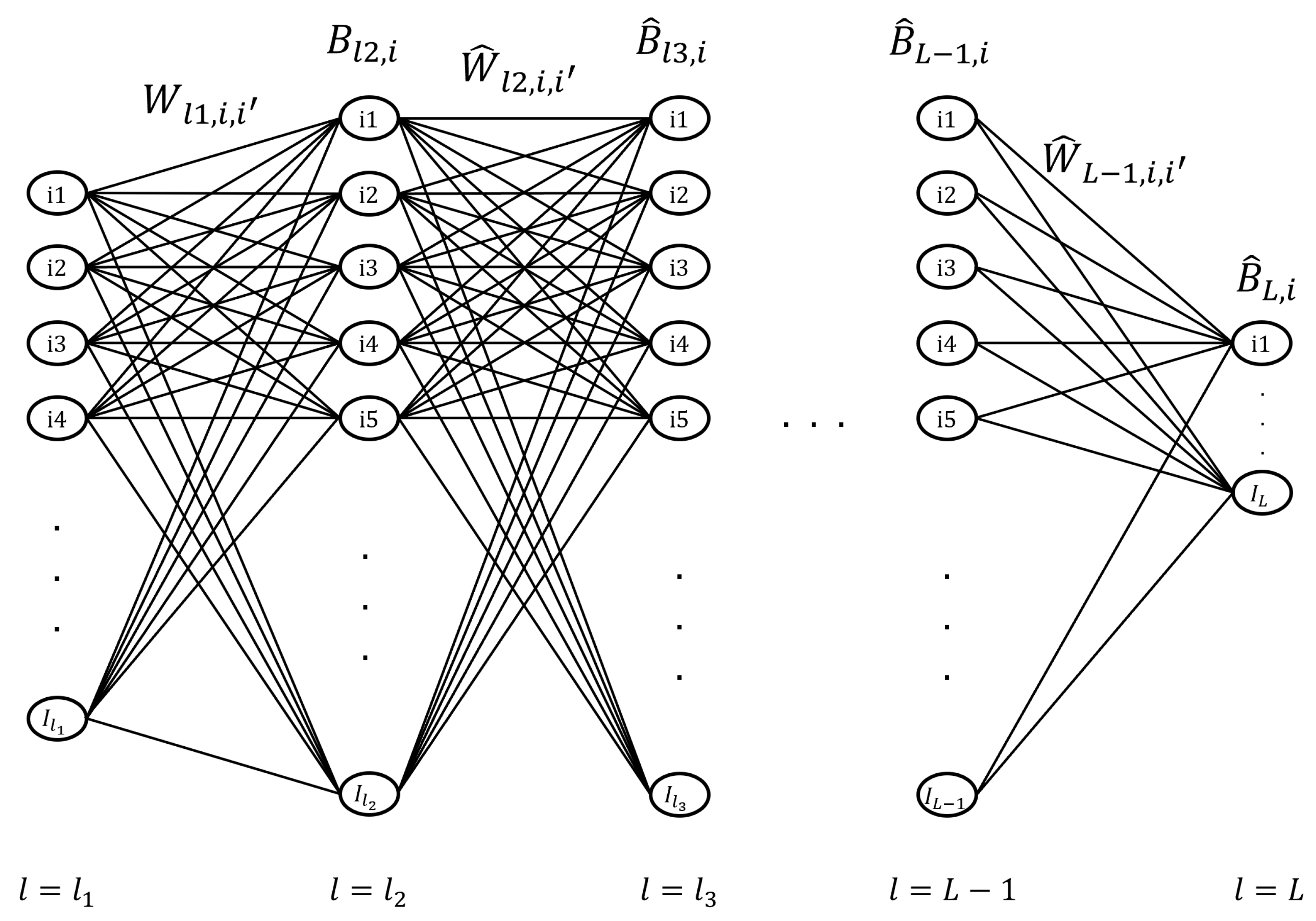
• The neural network is mathematically formulated, with the weights and biases of the first hidden layer treated as variables.
• The mathematical formulation is versatile enough to be applied to a deep neural network and can address multi-output regression datasets.
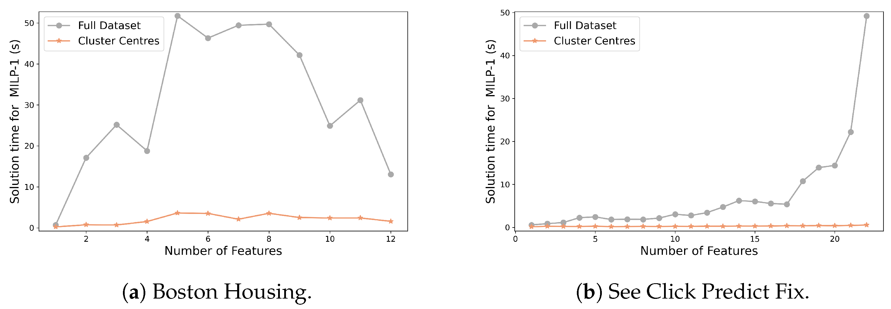
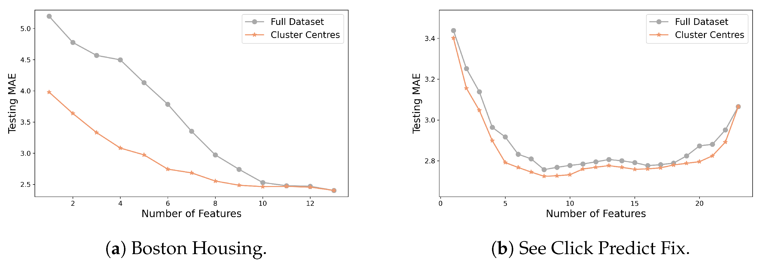
• Scalability is ensured by incorporating a clustering step to aggregate samples, enabling the approach to handle large datasets effectively.
• A specialised solution procedure is described, consisting of (i) clustering; (ii) mathematical programming; (iii) neural network training. This pipeline is employed in a recursive feature elimination manner.
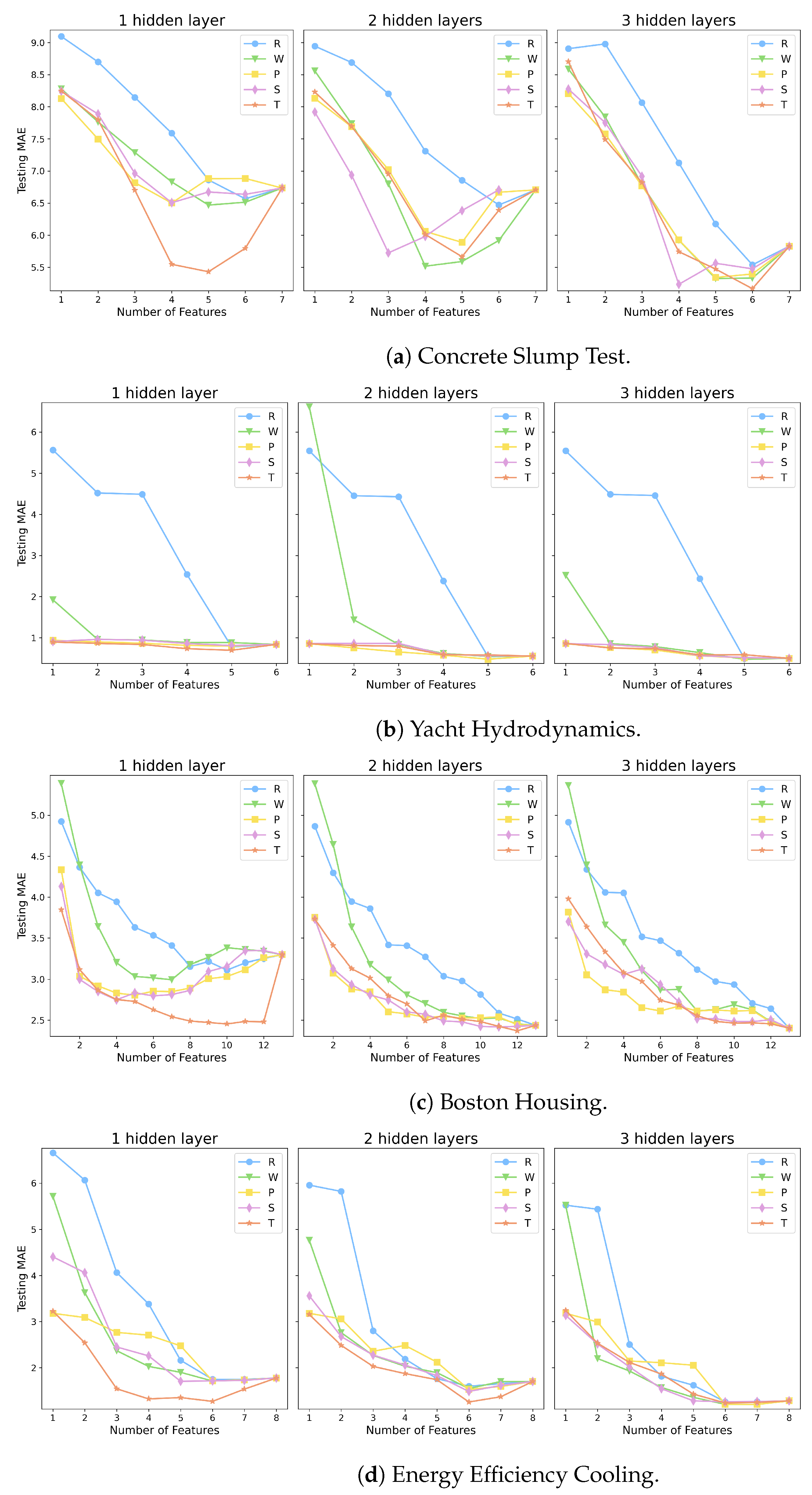
• A thorough computational comparison is performed against four other approaches, utilising eight datasets.

This paper is structured as follows: Section 2 presents the proposed approach, while Section 3 describes the implementation details. A number of benchmark regression datasets are employed to test the performance of our proposed method against other feature selection approaches and to demonstrate the explainability provided by the methodology. Finally, concluding remarks are provided in Section 4.

2. Methodology

2.1. Problem Statement

This section aims to introduce a feature selection methodology, namely TRUST, for regression neural networks that use a ReLU activation function. A pre-trained neural network is given with determined weights and biases. The MILP adjusts the weights and biases of the first hidden layer so that only a subset of the features is selected, while the connections (weights) for the remaining features are eliminated. The weights and biases of the next hidden layers are determined by the pre-trained neural network, and the number of selected features is determined by the user. For scalability reasons, a subset of the total number of samples is considered, determined by the k-medoids clustering method, which identifies cluster centres. The objective function minimises the absolute error of the cluster centres. Overall, the problem studied can be stated as follows:

• $Given:$

• The input values of C cluster centres with M features;
• The output values of C cluster centres;
• Determined weights and biases by the pre-trained neural network for all layers, l, from node i to node $i^{\prime }$;
• The number of features, $N_0$, that the selected subset should contain.

• $Determine:$

• Weights and biases for the first hidden layer from node i to node $i^{\prime }$;
• Selected features.

• $Soasto:$

• Minimise the summation of cluster centre errors, weighted by the percentage of samples in each cluster.

2.2. Mathematical Formulation

The indices, sets, parameters, and variables associated with the model are presented below:

Indices
m	Feature $(m=m_1,m_2,\dots ,M)$
l	Layer $(l=l_1,l_2,\dots ,L)$
$i,i^{\prime }$	Node $(i=i_1,i_2,\dots ,I)$
c	Cluster centre $(c=c_1,c_2,\dots ,C)$
Sets
$I_l$	Set of nodes that belong to layer l
$M_i$	Feature mapped to node i of input layer
Parameters
${\widehat{W}}_{l,i,i^{\prime }}$	Pre-trained weight of layer l between node i and node $i^{\prime }$
$W_{l,i,i^{\prime }}^{LO}$	Lower bound of weight in layer l between node i and node $i^{\prime }$
$W_{l,i,i^{\prime }}^{UP}$	Upper bound of weight in layer l between node i and node $i^{\prime }$
${\widehat{B}}_{li}$	Pre-trained bias in layer l for node i
$B_{li}^{LO}$	Lower bound of bias in layer l for node i
$B_{li}^{UP}$	Upper bound of bias in layer l for node i
${\widehat{x}}_{cli}$	Feature value of cluster centre c for input node i of first layer
$L{B}_{cli}$	Lower bound of input value for cluster centre c in layer l for node i
$U{B}_{cli}$	Upper bound of input value for cluster centre c in layer l for node i
$N_0$	Number of selected features
${\alpha }_c$	Coefficient of cluster centre c, representing percentage of samples in it
${\widehat{Y}}_{ci}$	Value of cluster centre c at output node i
Binary variables
${\sigma }_{cli}$	1, if input of cluster centre c in layer l for node i is positive; otherwise 0
$Z_m$	1, if feature m is selected; otherwise 0
Continuous variables
$x_{cli}$	Output of cluster centre c in layer l for node i
$D_{ci}$	Error for cluster centre c at output node i
$W_{l,i,i^{\prime }}$	Weight of layer l between node i and node $i^{\prime }$
$B_{li}$	Bias in layer l for node i

Figure 1 illustrates the general configuration of a fully connected feed-forward neural network, consisting of L layers, with the first layer as the input layer. Typically, the number of hidden layers and the number of nodes in each layer are user-defined and affect prediction quality significantly. A deep network is one with more than one hidden layer, and it is important to note that the proposed formulation is general enough to apply to neural networks with varying depths, being adaptable to different configurations. However, extending this approach to more complex architectures, such as convolutional or recurrent neural networks, would require developing specialised models tailored to their structural characteristics. The output layer is the final layer, with the number of nodes equal to the number of outputs in the dataset, which is more than one in the case of multi-output regression. In this structure, each layer, l, obtains the outputs from the previous layer, $l-1$, as the input. Within each hidden layer, the nodes calculate a weighted sum of their inputs. Then, an activation function is applied, which introduces nonlinearity into the model, and in this work, a ReLU activation function is considered. Although this study focuses on neural networks with ReLU activation functions, similar formulations can be developed for other activation functions. In general, a ReLU function is a piecewise linear function that will output the input directly if it is positive; otherwise, it will output zero:

$$\begin{array}{c}\hfill f\left(x\right)=max\{0,x\}\end{array}$$

This piecewise linear function is represented as a mixed-integer problem, and the big-M formulation can be employed to describe it [53]. In our model, the values for the big-M parameters are determined through interval arithmetic [54]. Starting with the first hidden layer, the weight from node i to node $i^{\prime }$, $W_{l_1,i,i^{\prime }}$, and the corresponding bias, $B_{l_2,i^{\prime }}$, are treated as variables. It is important to note that the input layer receives the input values of the cluster centres of the dataset, which are determined using k-medoids to reduce the model complexity. Constraints (1)–(3) work jointly in order to enforce the ReLU activation function in the first hidden layer. The output of node $i^{\prime }$, denoted as $x_{c,l+1,i^{\prime }}$, is equal to the input of the node, given by ${\sum }_{i\in I_l}(W_{l,i,i^{\prime }}·{\widehat{x}}_{c,l,i})+B_{l+1,i^{\prime }}$, when the binary variable ${\sigma }_{c,l+1,i^{\prime }}$ is equal to 1. This is enforced by Constraints (1) and (2). If ${\sigma }_{c,l+1,i^{\prime }}=0$, then the output is forced to become zero by Constraint (3). Here, it is worth noting that $L{B}_{c,l+1,i^{\prime }}$ and $U{B}_{c,l+1,i^{\prime }}$ are the lower and upper bounds of the input of node $i^{\prime }$, such that $L{B}_{c,l+1,i^{\prime }}\le {\sum }_{i\in I_l}(W_{l,i,i^{\prime }}·{\widehat{x}}_{c,l,i})+B_{l+1,i^{\prime }}\le U{B}_{c,l+1,i^{\prime }}$.

$$\begin{array}{c}\hfill \sum _{i\in I_l}(W_{l,i,i^{\prime }}·{\widehat{x}}_{c,l,i})+B_{l+1,i^{\prime }}\le x_{c,l+1,i^{\prime }}\forall c,l=l_1,i^{\prime }\in I_{l_2}\end{array}$$

(1)

$$\begin{array}{c}\hfill \begin{array}{c}\hfill \sum _{i\in I_l}(W_{l,i,i^{\prime }}·{\widehat{x}}_{c,l,i})+B_{l+1,i^{\prime }}-L{B}_{c,l+1,i^{\prime }}·(1-{\sigma }_{c,l+1,i^{\prime }})\ge x_{c,l+1,i^{\prime }}\\ \hfill \forall c,l=l_1,i^{\prime }\in I_{l_2}\end{array}\end{array}$$

(2)

$$\begin{array}{c}\hfill 0\le x_{cli}\le U{B}_{cli}·{\sigma }_{cli}\forall c,l:2\le l\le L-1,i\in I_l\end{array}$$

(3)

Similarly, the ReLU activation function for the subsequent hidden layers is expressed by Constraints (3)–(5). The key difference between the first hidden layer and subsequent ones is that the weights and biases in the latter are parameters (${\widehat{W}}_{l,i,i^{\prime }},{\widehat{B}}_{l,i}$) obtained from the pre-trained neural network.

$$\begin{array}{c}\hfill \sum _{i\in I_l}({\widehat{W}}_{l,i,i^{\prime }}·x_{c,l,i})+{\widehat{B}}_{l+1,i^{\prime }}\le x_{c,l+1,i^{\prime }}\forall c,l:2\le l\le L-2,i^{\prime }\in I_{l+1}\end{array}$$

(4)

$$\begin{array}{c}\hfill \begin{array}{c}\hfill \sum _{i\in I_l}({\widehat{W}}_{l,i,i^{\prime }}·x_{c,l,i})+{\widehat{B}}_{l+1,i^{\prime }}-L{B}_{c,l+1,i^{\prime }}·(1-{\sigma }_{c,l+1,i^{\prime }})\ge x_{c,l+1,i^{\prime }}\\ \hfill \forall c,l:2\le l\le L-2,i^{\prime }\in I_{l+1}\end{array}\end{array}$$

(5)

In the output layer, the nodes calculate a weighted summation of their inputs, as shown in Equation (6). Thus, no activation function is used for the output layer. Once again, the weights and biases used for the calculation of the weighted summation are parameters.

$$\begin{array}{c}\hfill x_{c,l,i^{\prime }}=\sum _{i\in I_{l-1}}({\widehat{W}}_{l-1,i,i^{\prime }}·x_{c,l-1,i})+{\widehat{B}}_{l,i^{\prime }}\forall c,l=L,i^{\prime }\in I_l\end{array}$$

(6)

Next, Constraints (7) and (8) are applied to enforce the selection of a subset of features from the original set. In Constraint (7), the weights of the first hidden layer are restricted to take values between $W_{l,i,i^{\prime }}^{LO}$ and $W_{l,i,i^{\prime }}^{UP}$ if the corresponding feature is selected and weights connected with the mapped input node are forced to zero, if a feature, m, is not selected. Constraint (8) restricts the number of selected features to a user-defined number, $N_0$.

$$\begin{array}{c}\hfill W_{l,i,i^{\prime }}^{LO}·Z_m\le W_{l,i,i^{\prime }}\le W_{l,i,i^{\prime }}^{UP}·Z_m\forall l=l_1,i\in I_{l_1},i^{\prime }\in I_{l_2},m\in M_i\end{array}$$

(7)

$$\begin{array}{c}\hfill \sum _m{Z}_m=N_0\end{array}$$

(8)

Then, Constraints (9) and (10) model the absolute deviation between the actual output, ${\widehat{Y}}_{ci}$, and the predicted output, $x_{cli}$, for all cluster centres, c, and output nodes, i.

$$\begin{array}{c}\hfill D_{ci}\ge {\widehat{Y}}_{ci}-x_{cli}\forall c,l=L,i\in I_l\end{array}$$

(9)

$$\begin{array}{c}\hfill D_{ci}\ge x_{cli}-{\widehat{Y}}_{ci}\forall c,l=L,i\in I_l\end{array}$$

(10)

The objective function aims to minimise the sum of the absolute errors of the cluster centres, each weighted by a coefficient, ${\alpha }_c$, which represents the percentage of samples in the corresponding cluster.

$$\begin{array}{c}\hfill min\sum _c{\alpha }_c·\sum _i{D}_{ci}\end{array}$$

(11)

The overall optimisation problem is formulated as an MILP model, which minimises (11) subject to Constraints (1)–(10). The objective function, as described in Equation (11), aims to minimise the summation of absolute errors of the cluster centers, weighted by the proportion of samples in each cluster. Simultaneously, the feature selection process, which is enforced by Constraints (7) and (8), ensures a reduction in the number of features by imposing a limit on the number of selected features, $N_0$, and setting unused feature weights to zero.

3. Computational Methodology

3.1. Sample Clustering

The number of samples in the MILP impacts its computational complexity, as the full set of samples leads to high resource requirements, limiting the scalability of the model. To enhance computational efficiency, we aimed to find the most representative samples of the dataset. Deciding the number of samples was a trade-off between the combinatorial complexity of the model and the accurate representation of the dataset. Here, k-medoids clustering was applied to the whole dataset using both features and outputs, in order to identify the most representative samples. The k-medoids method was chosen for its robustness to outliers and its ability to select actual data points as cluster representatives. This property was particularly beneficial in our approach, as retaining actual data points helped preserve meaningful feature relationships while reducing the dataset size [55,56].

Figure 2 shows the marginal relative inertia (mRI), which is defined in Appendix A, for different number of clusters for two datasets, namely See Click Predict Fix and Airfoil (two of the datasets used in our computational experiments in Section 3.2). It is noted that smaller log-scale figures in the top right corner provide additional context. It is observed that mRI decreases as the number of clusters increases. The chosen number of clusters should accurately represent the dataset while keeping the cluster cardinality low. A stopping criterion based on mRI ensures that only cluster centres that reduce the relative inertia (RI) by at least a specified threshold are retained. Although this is still a user-defined parameter, it contains a more intuitive expression to balance the trade-off. In the following experiments, a threshold of 0.5% for mRI was used as a stopping criterion in order to determine the number of clusters.

3.2. Computational Results

This section details how the applicability of the proposed approach, named TRUST (optimisaTion-based featuRe-selection for neUral-networks towardS explanabiliTy), was evaluated by testing it on several datasets. Implementation details are outlined in Figure 3, which illustrates the key steps for the recursive feature elimination algorithm. Although in the description of our algorithm in Section 2 the number of selected features is user-defined, in our computational experiments, features were systematically decreased until only one feature remained, for the purpose of comparing different feature selection methodologies across varying numbers of selected features. Firstly, the F parameter, representing the number of features considered, was initialised as equal to the total number of features in the examined dataset. Then, the neural network was trained in Tensorflow [57] using the training subset (80%). The prediction quality was assessed using the testing subset (20%) based on metrics: namely, MAE, MSE, $R^2$. The number of features considered, F, was checked so as to be greater than 1 and then updated to $F-1$. Moreover, k-medoids clustering was applied using all the features and outputs of the original dataset, and the cluster centres were identified. The reduction in the samples after clustering can be found in Appendix B. Meanwhile, the effect of clustering on both solution quality and time can be found in Appendix C. Afterwards, the weights and biases determined during the neural network training, along with the cluster centres determined by k-medoids, were passed to MILP-1. In MILP-1, the ranges of the first hidden-layer weights and biases were thus restricted to the values found during training (${\widehat{W}}_{l,i,i^{\prime }},{\widehat{B}}_{l,i}$):

• $W_{l,i,i^{\prime }}^{LO}=W_{l,i,i^{\prime }}^{UP}={\widehat{W}}_{l,i,i^{\prime }}$
• $B_{l,i}^{LO}=B_{l,i}^{UP}={\widehat{B}}_{l,i}$

The number of selected features, denoted as $N_0$ in the mathematical model, is a user-defined number. In this case, it was set as equal to $F-1$. The restriction of the ranges of the weights and biases reduced the search space and resulted in a globally optimal solution. This solution was injected as a warm start before starting the solver in order to boost the performance of MILP-2, which had a larger search space. Specifically, the lower and upper bounds for the first hidden-layer weights and biases in MILP-2 were as follows:

• $W_{l,i,i^{\prime }}^{LO}=-2·\left|{\widehat{W}}_{l,i,i^{\prime }}\right|$
• $W_{l,i,i^{\prime }}^{UP}=2·\left|{\widehat{W}}_{l,i,i^{\prime }}\right|$
• $B_{l,i}^{LO}=-2·\left|{\widehat{B}}_{l,i}\right|$
• $B_{l,i}^{UP}=2·\left|{\widehat{B}}_{l,i}\right|$

In this way, MILP-2 was also solved for $N_0=F-1$. The time limit was set as equal to 60 s. This allowed the least important feature to be selected, and the new weights and biases for the first hidden layer were determined. In the next step, the weights and biases were given as initialisation for the next training of the neural network that used the subset of selected features. This procedure was terminated when $F=1$. The proposed algorithm was run 15 times for different training–testing splits in order to obtain the average testing metrics.

Feature values in the various datasets were normalised by first fitting the scaler to the training set only to avoid data leakage, and then the scaler parameters were applied to transform the testing set. The same training and testing subsets were used across all approaches during each iteration. Importantly, the neural network, initially trained using all the features, remained the same for all the feature selection approaches.

The MILP implementation was performed with the mathematical optimisation package GAMSPy (General Algebraic Modeling System—Python) [58] with GUROBI [59] as the selected solver. Moreover, the optimality gap was set as equal to 1%. For the neural network training in Tensorflow, a ReLU activation function and the Adam optimiser [60] are employed. Regarding the neural network architecture, three different configurations were examined, consisting of one, two, and three hidden layers containing 10 hidden nodes each. The proposed methodology was applied to a number of datasets that are widely used as benchmarks for comparing the performance of various regression methods, shown in

Table 1. A description of the datasets used in the experiments.

Dataset	Abbreviation	Samples	Features	Outputs
Concrete Slump Test	CST	103	7	3
Yacht Hydrodynamics	YH	308	6	1
Boston Housing	BH	506	13	1
Energy Efficiency Cooling	EEC	768	8	1
Energy Efficiency Heating	EEH	768	8	1
Energy Efficiency Both	EEB	768	8	2
See Click Predict Fix	SCPF	1137	23	3
Airfoil	AF	1503	5	1

, and comparisons with other feature selection techniques are reported. The neural networks were trained using the same hyper-parameters and initialisation across all approaches in order to ensure a fair comparison.

The Boston Housing dataset is available through Statlib [61], the See Click Predict Fix dataset can be found in Mulan library [62], and the rest of the datasets can be downloaded from UCI machine learning repository [63]. The Concrete Slump Test dataset predicts the slump, flow, and 28-day compressive strength of concrete based on the quantities of its components. The Yacht Hydrodynamics dataset is used to predict the residuary resistance of sailing yachts during the initial design stage to evaluate their performance. The Boston Housing dataset consists of observations used to predict house prices in suburbs of Boston. In Energy Efficiency Cooling and Energy Efficiency Heating, the cooling and heating load requirements of buildings are predicted based on their shape characteristics. The Energy Efficiency Both dataset examines the combined outputs of heating and cooling load predictions. In See Click Predict Fix, data from 311 service reports of various U.S. cities are used and the task is to predict the number of views, clicks, and comments received by issues such as potholes, graffiti, and trash. The features include the type of issue, report source, location, and duration the issue remains online. Finally, the Airfoil dataset contains data obtained from a series of aerodynamic and acoustic tests conducted by NASA in an anechoic wind tunnel. The sound pressure level is predicted using airfoil design parameters.

The approaches that were considered for comparison were Random feature selection, Weight feature selection, Pearson feature selection, and SHAP feature selection. Random feature selection randomly selected a subset of features, serving as a baseline for comparison in the experiments. In Weight feature selection, a subset of features was selected based on the weights of the trained neural network. More specifically, the summation of the absolute values of all weights connecting each input node to the nodes in the next layer was calculated. The inputs associated with the highest summations were then selected, since the inputs linked to small weights were less likely to be important, having less influence on the neural network prediction [36]. For the next feature selection methodology, the Pearson correlation coefficient was computed between each feature and the output [64]. The features that had high absolute values of Pearson correlation coefficients were considered highly correlated with the output and were selected. In the case of multiple outputs, the absolute values of the Pearson correlation coefficients of each output were summed, and the features with the highest total values were selected. Finally, SHAP (SHapley Additive exPlanations) was used as a feature selection methodology. It uses a game theoretic approach to calculate the contribution of each feature to the model predictions by attributing Shapley values [22]. These values are computed by considering all possible subsets of features and measuring the marginal contribution of each feature to the model output across different combinations. In the experiments, the features with the highest SHAP values were selected, as they were identified as the most impactful for determining the model outputs. All runs for comparing feature selection approaches followed the same recursive feature elimination procedure, removing features one by one, as previously described in our approach, so as to ensure a fair comparison across different feature selection techniques.

Figure 4 and Figure 5 illustrate the average Mean Absolute Error (MAE) of the Random, Weight, Pearson, SHAP, and TRUST approaches for all examined datasets against the number of features. Neural network configurations with one, two, and three hidden layers, each with 10 hidden nodes, were considered and reported. As the neural networks were initialised identically, all methodologies began from the same point, when using the full set of features for training. When one hidden layer was used, TRUST outperformed all other approaches in most datasets. Specifically, for the YH, BH, EEC, EEH, and EEB datasets, TRUST exhibited the lowest average MAE for nearly all feature counts. As expected, Random feature selection clearly showed the worst predictive performance among the examined methodologies with the highest average MAE for the most numbers of features examined, indicating the importance of selecting the best subset of features. As far as the Weight, Pearson, and SHAP methodologies were concerned, they generally fell between the Random and TRUST approaches in performance. In most datasets, they alternated with varying feature counts, and it was difficult to identify a clear winner. In the neural network configuration with two hidden layers, TRUST exhibited the best predictive performance in most cases, particularly in the EEC, EEH, and SCPF datasets. Finally, for three hidden layers, once again, TRUST showed competitive performance, especially in the YH, EEB, and SCPF datasets.

Generating rankings based on algorithm performance on related datasets was also used to compare the performance across methodologies. A scoring strategy was employed where the best-performing method received five points, the worst performer was awarded one point, and the average score of each method across all datasets was used to rank them. Figure 6 shows the rankings for all neural network configurations and testing metrics. Our key finding was that TRUST consistently outscored other methodologies across all configurations and testing metrics. Pearson feature selection ranked second for one- and two-hidden-layer configurations across all metrics, followed by SHAP and Weight feature selection. SHAP performed better in the three-hidden-layer configuration but was still below TRUST. Random feature selection consistently ranked last but served as a useful baseline for comparison. Overall, the rankings demonstrated that TRUST consistently delivered high predictive performance, surpassing the other approaches in the majority of cases and highlighting the advantages conferred by our methodology.

TRUST enhances neural network explainability by identifying important features for prediction quality. Neural networks are often seen as black boxes but TRUST elucidates feature importance in prediction via the key binary variable of the MILP, $Z_m$, which determines the subset of selected features. As depicted in Figure 3, in each iteration, one feature was removed until one remained and the frequency with which a feature was retained provided a measure of its importance. Therefore, the average number of times each feature was selected during the feature elimination process was calculated and Figure 7 and Figure 8 display the average selection frequency of each feature as a percentage. It follows that a feature selection frequency of 100% indicates cases where a feature was the last one to remain and a selection frequency of 0% means that the feature was always the first to be removed. The full names and descriptions of all features are provided in Appendix D for reference.

For Concrete Slump Test dataset, Water Concentration (WC) was consistently the most important feature, while Superplasticiser Concentration (SC) was the least selected, indicating strong consensus across neural network configurations. In the Yacht Hydrodynamics dataset, Froude number (FN) was consistently the most influential, while the least selected features varied: the Prismatic Coefficient (PC) for one hidden layer and Longitudinal Position of the Centre of Buoyancy (LPCB) for two and three hidden layers. In the Boston Housing dataset, house prices were most influenced by the percentage of lower-status population (LSTAT), while the Proportion of Residential Land Zoned for Large Lots (ZN) and the Proximity to the Charles River (CHAS) were least influential. Similarly, in the Energy Efficiency Cooling, Energy Efficiency Heating, and combined dataset, there was agreement that Overall Height (OH) was the most important feature, while Orientation (O) and Glazing Area Distribution (GAD) were the least important. The most influential features in the See Click Predict Fix dataset were the number of days online (NOD), remote API (SR), the issue being trash (ITS), and whether the city was Richmond (CR). For the Airfoil dataset, the most critical features were the frequency (F) and the Suction Side Displacement Thickness (SSD), whereas the least important was the Free Stream Velocity (FSV). Overall, these findings underscore the valuable insights that TRUST was able to reveal with consistent rankings regardless of the number of hidden layers in the neural network configuration.

4. Conclusions

In this work, we propose an optimisation-based feature selection methodology for neural networks, named TRUST. Designed for regression neural networks with ReLU activation functions, TRUST leverages a trained neural network to identify the most important features by adjusting the weights and biases of the first hidden layer. It is formulated mathematically as a Mixed-Integer Linear Programming (MILP) model and the complexity is reduced using k-medoids clustering as a pre-processing step. The applicability of the proposed methodology was demonstrated through a number of regression datasets from the literature. Computational results indicate that neural networks achieved superior performance when trained on subsets of features selected by TRUST compared to other feature selection methods. This competitiveness was consistent across different neural network configurations and prediction quality metrics. Additionally, the MILP solution contributes to Explainable Artificial Intelligence (XAI) by quantifying feature importance through the frequency of selection of each feature, offering valuable insights into the influence on model predictions. Overall, the computational results highlight the suitability of our approach for real-world datasets when the goal is to select a subset of features in order to achieve low prediction error, while also gaining insights about the features and their contribution to the predictions of the model. Future work can explore improving the scalability of the approach for high-dimensional datasets, as increasing features may impact computational performance. Meanwhile, the decision of the final number of features, if not determined by the user, could be guided by the employment of an information criterion, which constitutes another research direction.

References

1. Hastie, T.; Tibshirani, R.; Friedman, J. The Elements of Statistical Learning; Springer Series in Statistics; Springer: Berlin/Heidelberg, Germany, 2008. [Google Scholar]
2. Draper, N.R.; Smith, H. Applied Regression Analysis; Wiley: New York, NY, USA, 1998. [Google Scholar]
3. Tibshirani, R. Regression Shrinkage and Selection via the Lasso. J. R. Stat. Soc. 1996, 58, 267–288. [Google Scholar] [CrossRef]
4. Breiman, L.; Friedman, J.H.; Olshen, R.A.; Stone, C.J. Classification and Regression Trees; Taylor & Francis: New York, NY, USA, 1984. [Google Scholar] [CrossRef]
5. Breiman, L. Random Forests. Mach. Learn. 2001, 45, 5–32. [Google Scholar] [CrossRef]
6. Cortes, C.; Vapnik, V.; Saitta, L. Support-Vector Networks. Mach. Learn. 1995, 20, 273–297. [Google Scholar] [CrossRef]
7. Rio-Chanona, E.A.D.; Wagner, J.L.; Ali, H.; Fiorelli, F.; Zhang, D.; Hellgardt, K. Deep learning-based surrogate modeling and optimization for microalgal biofuel production and photobioreactor design. AIChE J. 2019, 65, 915–923. [Google Scholar] [CrossRef]
8. Panerati, J.; Schnellmann, M.A.; Patience, C.; Beltrame, G.; Patience, G.S. Experimental methods in chemical engineering: Artificial neural networks—ANNs. Can. J. Chem. Eng. 2019, 97, 2372–2382. [Google Scholar] [CrossRef]
9. Sildir, H.; Aydin, E. A Mixed-Integer linear programming based training and feature selection method for artificial neural networks using piece-wise linear approximations. Chem. Eng. Sci. 2022, 249, 117273. [Google Scholar] [CrossRef]
10. Shah, V.; Konda, S.R. Neural Networks and Explainable AI: Bridging the Gap between Models and Interpretability. Int. J. Comput. Sci. Technol. 2021, 5, 2. [Google Scholar] [CrossRef]
11. Camburu, O.M. Explaining Deep Neural Networks. arXiv 2020, arXiv:2010.01496. [Google Scholar]
12. Bienefeld, N.; Boss, J.M.; Lüthy, R.; Brodbeck, D.; Azzati, J.; Blaser, M.; Willms, J.; Keller, E. Solving the explainable AI conundrum by bridging clinicians’ needs and developers’ goals. Digit. Med. 2023, 6, 94. [Google Scholar] [CrossRef]
13. Chaddad, A.; Peng, J.; Xu, J.; Bouridane, A. Survey of Explainable AI Techniques in Healthcare. Sensors 2023, 23, 634. [Google Scholar] [CrossRef]
14. Li, Y.; Cardoso-Silva, J.; Kelly, J.M.; Delves, M.J.; Furnham, N.; Papageorgiou, L.G.; Tsoka, S. Optimisation-based modelling for explainable lead discovery in malaria. Artif. Intell. Med. 2024, 147, 102700. [Google Scholar] [CrossRef]
15. Alghamdi, F.A.; Almanaseer, H.; Jaradat, G.; Jaradat, A.; Alsmadi, M.K.; Jawarneh, S.; Almurayh, A.S.; Alqurni, J.; Alfagham, H. Multilayer Perceptron Neural Network with Arithmetic Optimization Algorithm-Based Feature Selection for Cardiovascular Disease Prediction. Mach. Learn. Knowl. Extr. 2024, 6, 987–1008. [Google Scholar] [CrossRef]
16. Papadopoulos, S.; Kontokosta, C.E. Grading buildings on energy performance using city benchmarking data. Appl. Energy 2019, 233, 244–253. [Google Scholar] [CrossRef]
17. Letzgus, S.; Wagner, P.; Lederer, J.; Samek, W.; Muller, K.R.; Montavon, G. Toward Explainable Artificial Intelligence for Regression Models: A methodological perspective. IEEE Signal Process. Mag. 2022, 39, 40–58. [Google Scholar] [CrossRef]
18. Wheeler, A.P.; Steenbeek, W. Mapping the Risk Terrain for Crime Using Machine Learning. J. Quant. Criminol. 2021, 37, 445–480. [Google Scholar] [CrossRef]
19. Marcinkevičs, R.; Vogt, J.E. Interpretable and explainable machine learning: A methods-centric overview with concrete examples. Wiley Interdiscip. Rev. Data Min. Knowl. Discov. 2023, 13, e1493. [Google Scholar] [CrossRef]
20. Rudin, C. Stop explaining black box machine learning models for high stakes decisions and use interpretable models instead. Nat. Mach. Intell. 2019, 1, 206–215. [Google Scholar] [CrossRef]
21. Goerigk, M.; Hartisch, M. A framework for inherently interpretable optimization models. Eur. J. Oper. Res. 2023, 310, 1312–1324. [Google Scholar] [CrossRef]
22. Lundberg, S.; Lee, S.I. A Unified Approach to Interpreting Model Predictions. arXiv 2017, arXiv:1705.07874. [Google Scholar]
23. Ribeiro, M.T.; Singh, S.; Guestrin, C. Why Should I Trust You? In Proceedings of the 22nd ACM SIGKDD International Conference on Knowledge Discovery and Data Mining, San Francisco, CA, USA, 13–17 August 2016; pp. 1135–1144. [Google Scholar] [CrossRef]
24. Janzing, D.; Minorics, L.; Blöbaum, P. Feature relevance quantification in explainable AI: A causality problem. arXiv 2019, arXiv:1910.13413. [Google Scholar]
25. Jiménez-Luna, J.; Grisoni, F.; Schneider, G. Drug discovery with explainable artificial intelligence. Nat. Mach. Intell. 2020, 2, 573–584. [Google Scholar] [CrossRef]
26. Zafar, M.R.; Khan, N. Deterministic Local Interpretable Model-Agnostic Explanations for Stable Explainability. Mach. Learn. Knowl. Extr. 2021, 3, 525–541. [Google Scholar] [CrossRef]
27. Li, J.; Cheng, K.; Wang, S.; Morstatter, F.; Trevino, R.P.; Tang, J.; Liu, H. Feature Selection. ACM Comput. Surv. 2018, 50, 1–45. [Google Scholar] [CrossRef]
28. Clautiaux, F.; Ljubić, I. Last fifty years of integer linear programming: A focus on recent practical advances. Eur. J. Oper. Res. 2024. [Google Scholar] [CrossRef]
29. Huchette, J.; Muñoz, G.; Serra, T.; Tsay, C. When Deep Learning Meets Polyhedral Theory: A Survey. arXiv 2023, arXiv:2305.00241. [Google Scholar]
30. Fischetti, M.; Jo, J. Deep neural networks and mixed integer linear optimization. Constraints 2018, 23, 296–309. [Google Scholar] [CrossRef]
31. Tjeng, V.; Xiao, K.; Tedrake, R. Evaluating Robustness of Neural Networks with Mixed Integer Programming. arXiv 2019, arXiv:1711.07356. [Google Scholar]
32. Dias, L.S.; Ierapetritou, M.G. Data-driven feasibility analysis for the integration of planning and scheduling problems. Optim. Eng. 2019, 20, 1029–1066. [Google Scholar] [CrossRef]
33. Dias, L.S.; Ierapetritou, M.G. Integration of planning, scheduling and control problems using data-driven feasibility analysis and surrogate models. Comput. Chem. Eng. 2020, 134, 106714. [Google Scholar] [CrossRef]
34. Triantafyllou, N.; Papathanasiou, M.M. Deep learning enhanced mixed integer optimization: Learning to reduce model dimensionality. Comput. Chem. Eng. 2024, 187, 108725. [Google Scholar] [CrossRef]
35. López-Flores, F.J.; Lira-Barragán, L.F.; Rubio-Castro, E.; El-Halwagi, M.M.; Ponce-Ortega, J.M. Hybrid Machine Learning-Mathematical Programming Approach for Optimizing Gas Production and Water Management in Shale Gas Fields. ACS Sustain. Chem. Eng. 2023, 11, 6043–6056. [Google Scholar] [CrossRef]
36. Zhao, S.; Tsay, C.; Kronqvist, J. Model-based feature selection for neural networks: A mixed-integer programming approach. arXiv 2023, arXiv:2302.10344. [Google Scholar]
37. Carrizosa, E.; Ramírez-Ayerbe, J.; Romero Morales, D. Mathematical optimization modelling for group counterfactual explanations. Eur. J. Oper. Res. 2024, 319, 399–412. [Google Scholar] [CrossRef]
38. Lodi, A.; Ramírez-Ayerbe, J. One-for-many Counterfactual Explanations by Column Generation. arXiv 2024, arXiv:2402.09473. [Google Scholar]
39. Bertsimas, D.; Dunn, J. Optimal classification trees. Mach. Learn. 2017, 106, 1039–1082. [Google Scholar] [CrossRef]
40. Verwer, S.; Zhang, Y.; Ye, Q.C. Auction optimization using regression trees and linear models as integer programs. Artif. Intell. 2017, 244, 368–395. [Google Scholar] [CrossRef]
41. Gkioulekas, I.; Papageorgiou, L.G. Tree regression models using statistical testing and mixed integer programming. Comput. Ind. Eng. 2021, 153, 107059. [Google Scholar] [CrossRef]
42. Liapis, G.I.; Papageorgiou, L.G. Optimisation-Based Classification Tree: A Game Theoretic Approach to Group Fairness. Commun. Comput. Inf. Sci. 2025, 2311, 28–40. [Google Scholar] [CrossRef]
43. Carrizosa, E.; Martin-Barragan, B. Two-group classification via a biobjective margin maximization model. Eur. J. Oper. Res. 2006, 173, 746–761. [Google Scholar] [CrossRef]
44. Carrizosa, E.; Morales, D.R. Supervised classification and mathematical optimization. Comput. Oper. Res. 2013, 40, 150–165. [Google Scholar] [CrossRef]
45. Blanco, V.; Japón, A.; Puerto, J. A mathematical programming approach to SVM-based classification with label noise. Comput. Ind. Eng. 2022, 172, 108611. [Google Scholar] [CrossRef]
46. Liapis, G.I.; Papageorgiou, L.G. Hyper-box Classification Model Using Mathematical Programming. Lect. Notes Comput. Sci. 2023, 14286, 16–30. [Google Scholar] [CrossRef]
47. Liapis, G.I.; Tsoka, S.; Papageorgiou, L.G. Interpretable optimisation-based approach for hyper-box classification. Mach. Learn. 2025, 114, 51. [Google Scholar] [CrossRef]
48. Rosenberg, G.; Brubaker, J.K.; Schuetz, M.J.A.; Salton, G.; Zhu, Z.; Zhu, E.Y.; Kadıoğlu, S.; Borujeni, S.E.; Katzgraber, H.G. Explainable Artificial Intelligence Using Expressive Boolean Formulas. Mach. Learn. Knowl. Extr. 2023, 5, 1760–1795. [Google Scholar] [CrossRef]
49. Toro Icarte, R.; Illanes, L.; Castro, M.P.; Cire, A.A.; McIlraith, S.A.; Beck, J.C. Training Binarized Neural Networks Using MIP and CP. In Proceedings of the Principles and Practice of Constraint Programming, Stamford, CT, USA, 30 September–4 October 2019; Springer International Publishing: Cham, Switzerland, 2019; pp. 401–417. [Google Scholar]
50. Thorbjarnarson, T.; Yorke-Smith, N. Optimal training of integer-valued neural networks with mixed integer programming. PLoS ONE 2023, 18, e0261029. [Google Scholar] [CrossRef]
51. Dua, V. A mixed-integer programming approach for optimal configuration of artificial neural networks. Chem. Eng. Res. Des. 2010, 88, 55–60. [Google Scholar] [CrossRef]
52. Park, H.S.; Jun, C.H. A simple and fast algorithm for K-medoids clustering. Expert Syst. Appl. 2009, 36, 3336–3341. [Google Scholar] [CrossRef]
53. Cheng, C.H.; Nührenberg, G.; Ruess, H. Maximum Resilience of Artificial Neural Networks. arXiv 2017, arXiv:1705.01040. [Google Scholar]
54. Tsay, C.; Kronqvist, J.; Thebelt, A.; Misener, R. Partition-based formulations for mixed-integer optimization of trained ReLU neural networks. arXiv 2021, arXiv:2102.04373. [Google Scholar]
55. Madhulatha, T.S. Comparison between K-Means and K-Medoids Clustering Algorithms. In Proceedings of the Advances in Computing and Information Technology, Chennai, India, 15–17 July 2011; pp. 472–481. [Google Scholar] [CrossRef]
56. Arora, P.; Deepali; Varshney, S. Analysis of K-Means and K-Medoids Algorithm For Big Data. Procedia Comput. Sci. 2016, 78, 507–512. [Google Scholar] [CrossRef]
57. Abadi, M.; Agarwal, A.; Barham, P.; Brevdo, E.; Chen, Z.; Citro, C.; Corrado, G.S.; Davis, A.; Dean, J.; Devin, M.; et al. TensorFlow: Large-Scale Machine Learning on Heterogeneous Systems. 2015. Available online: http://tensorflow.org (accessed on 1 February 2025).
58. GAMS Development Corporation. General Algebraic Model System (GAMS); Release 46.1.0; GAMS Development Corporation: Washington, DC, USA, 2024. [Google Scholar]
59. Gurobi Optimization, LLC. Gurobi Optimizer Reference Manual. 2024. Available online: https://www.gurobi.com (accessed on 1 February 2025).
60. Kingma, D.P.; Ba, J. Adam: A Method for Stochastic Optimization. arXiv 2014, arXiv:1412.6980. [Google Scholar]
61. Vlachos, P. StatLib—Statistical Datasets. 2005. Available online: http://lib.stat.cmu.edu/datasets/ (accessed on 1 February 2025).
62. Tsoumakas, G.; Spyromitros-Xioufis, E.; Vilcek, J.; Vlahavas, I. Mulan: A Java Library for Multi-Label Learning. J. Mach. Learn. Res. 2011, 12, 2411–2414. [Google Scholar]
63. Dua, D.; Graff, C. UCI Machine Learning Repository. 2017. Available online: http://archive.ics.uci.edu/ml/index.php (accessed on 1 February 2025).
64. Virtanen, P.; Gommers, R.; Oliphant, T.E.; Haberland, M.; Reddy, T.; Cournapeau, D.; Burovski, E.; Peterson, P.; Weckesser, W.; Bright, J.; et al. SciPy 1.0: Fundamental Algorithms for Scientific Computing in Python. Nat. Methods 2020, 17, 261–272. [Google Scholar] [CrossRef] [PubMed]
65. Herding, R.; Ross, E.; Jones, W.R.; Endler, E.; Charitopoulos, V.M.; Papageorgiou, L.G. Risk-aware microgrid operation and participation in the day-ahead electricity market. Adv. Appl. Energy 2024, 15, 100180. [Google Scholar] [CrossRef]
Figure 1. A schematic representation of a fully connected feed-forward neural network configuration illustrating weights and biases.
Make 07 00033 g001
Figure 2. Marginal relative inertia (mRI) for different cardinalities of clusters in k-medoids clustering for See Click Predict Fix and Airfoil datasets.
Make 07 00033 g002
Figure 3. A schematic representation of the TRUST algorithm.
Make 07 00033 g003
Figure 4. Average MAE of Random, Weight, Pearson, SHAP, and TRUST for different number of features across first four examined datasets.
Make 07 00033 g004
Figure 5. Average MAE of Random, Weight, Pearson, SHAP, and TRUST for different number of features across last four examined datasets.
Make 07 00033 g005
Figure 6. Average performance rankings of Random, Weight, Pearson, SHAP, and TRUST across neural network configurations and testing metrics.
Make 07 00033 g006
Figure 7. Average percentage of times that each feature was selected by TRUST for first four examined datasets.
Make 07 00033 g007
Figure 8. Average percentage of times that each feature was selected by TRUST for last four examined datasets.
Make 07 00033 g008