Article

Efficient Visual-Aware Fashion Recommendation Using Compressed Node Features and Graph-Based Learning

by
Umar Subhan Malhi
1,
Junfeng Zhou
1,*,
Abdur Rasool
2 and
Shahbaz Siddeeq
3
1
School of Computer Science and Technology, Donghua University, Songjiang, Shanghai 200051, China
2
Department of Information and Computer Sciences, University of Hawaii at Manoa, Honolulu, HI 96822, USA
3
Faculty of Information Technology and Communication Sciences, Tampere University, 33100 Tampere, Finland
*
Author to whom correspondence should be addressed.
Mach. Learn. Knowl. Extr. 2024, 6(3), 2111-2129; https://doi.org/10.3390/make6030104
Submission received: 14 August 2024 / Revised: 6 September 2024 / Accepted: 12 September 2024 / Published: 15 September 2024
(This article belongs to the Special Issue Machine Learning in Data Science)

Abstract

:
In fashion e-commerce, predicting item compatibility using visual features remains a significant challenge. Current recommendation systems often struggle to incorporate high-dimensional visual data into graph-based learning models effectively. This limitation presents a substantial opportunity to enhance the precision and effectiveness of fashion recommendations. In this paper, we present the Visual-aware Graph Convolutional Network (VAGCN). This novel framework helps improve how visual features can be incorporated into graph-based learning systems for fashion item compatibility predictions. The VAGCN framework employs a deep-stacked autoencoder to convert the input image’s high-dimensional raw CNN visual features into more manageable low-dimensional representations. In addition to improving feature representation, the GCN can also reason more intelligently about predictions, which would not be possible without this compression. The GCN encoder processes nodes in the graph to capture structural and feature correlation. Following the GCN encoder, the refined embeddings are input to a multi-layer perceptron (MLP) to calculate compatibility scores. The approach extends to using neighborhood information only during the testing phase to help with training efficiency and generalizability in practical scenarios, a key characteristic of our model. By leveraging its ability to capture latent visual features and neighborhood-based learning, VAGCN thoroughly investigates item compatibility across various categories. This method significantly improves predictive accuracy, consistently outperforming existing benchmarks. These contributions tackle significant scalability and computational efficiency challenges, showcasing the potential transformation of recommendation systems through enhanced feature representation, paving the way for further innovations in the fashion domain.

1. Introduction

Fashion recommendation systems (FRS) have become indispensable tools to increase user engagement and satisfaction by providing a personalized shopping experience [1,2]. Traditional recommendation systems (RSs) have relied on user behaviors, such as viewing client activity, purchase history, click-through rate, navigating habits, etc., to suggest products that resonate with user preferences [3,4]. However, these systems often overlook the full spectrum of available data, mainly the visual information essential for fashion items, and are decisive in suggesting outfits that are both visually compelling and aesthetically appealing [5].
As e-commerce platforms continue to expand, there is a need for more scalable methods to solve such problems, such as link prediction within RSs. Link prediction, mainly when applied through graph neural networks (GNNs), is essential for enhancing the capabilities of recommendation systems [6]. It involves predicting the likelihood of a relationship between two nodes in a graph, which, in the context of fashion, translates to the compatibility between items. This technique is more powerful than traditional recommendations. It has broad applications beyond recommendation, particularly in solving challenging problems like the sponsored search problem found on web platforms, where modeling and understanding complex relationships among items can profoundly impact the relevance and effectiveness of search results [7]. By leveraging GNNs for link prediction, FRS can adopt a more nuanced approach that considers user history and the intricate visual relationships between fashion items, thus bridging the gap between user preferences and item compatibility [8].
GNNs help RS perceive diverse relationships more effectively in large networks [9]. In fashion e-commerce, GNNs have excellent potential to model user-item transactions and item-item interactions collectively. This capability allows GNNs to perform a multi-dimensional comparison of similarities between items in style, color, and fabric [10]. Integrating GNNs enables a deeper understanding of product compatibilities, enhancing recommendations by identifying the intrinsic patterns that drive fashion trends and consumer preferences [11]. Although GNNs bring significant benefits to FRS, the complexity of high-dimensional data is still a bottleneck in modern AI systems, and most cases of graph-based learning are used in e-commerce platforms [12,13]. Traditional GCNs, while effective, often scale poorly to the large datasets characteristic of many such environments [14]. This limitation is mostly because of the difficulty of directly embedding high-dimensional visual features into the structure of the graph needed for capturing the information content of the visual data [15,16,17].
To address these challenges with FRS, our study introduces the VAGCN, a model that enhances graph-based learning frameworks by incorporating advanced visual feature extraction techniques. First, we reduce the high-dimensional CNN features to a compact, low-dimensional latent space via a deep autoencoder architecture. In addition to its utility in assisting with the curse of dimensionality [18,19], this step retains the most important features that provide deeper insight for a refined relationship of item compatibility [20]. Given the results from our previous work, which empirically found highly significant performance enhancement in clustering by compressed feature maps [21,22], our approach extends these benefits to compatibility assessments and fashion item recommendations. By embedding these compressed features directly into a GCN’s graph structure during pre-training, it refines such selection with advanced denoising techniques to ensure that the visual data strongly interacts with the model’s predictive capabilities. The proposed VAGCN can effectively process large-scale graph data and enhance prediction accuracy by incorporating neighborhood information during testing. This integration enables the VAGCN to interpret complex inter-item relationships effectively, producing compatibility predictions closely aligned with visual preferences influencing consumer behavior in fashion e-commerce. This paper advances the field of fashion recommendation systems through several key contributions:
  • We introduce the VAGCN, which utilizes enhanced visual features in the graph-based learning process to improve the model’s understanding of complex product relationships.
  • We develop a sophisticated graph-based model that leverages compressed node features via a deep-stacked autoencoder. This approach reduces computational load while integrating latent visual data, enabling a comprehensive analysis of fashion item compatibility.
  • We optimize the GCN architecture by decreasing hidden units across layers, balancing efficiency and accuracy.
  • We investigate the impact of neighborhood size on the effectiveness of graph-based learning, providing evidence to optimize the balance between accuracy and computational efficiency.
  • We demonstrate the effectiveness of the VAGCN through rigorous validation across various fashion categories, comparing its performance with existing methods.
We organize the rest of the paper as follows: Section 2 discusses related work and identifies FRS gaps using graph-based methods. Section 3 details the methodology, elaborating on the VAGCN architecture and the integration of enhanced visual features. Section 4 discusses the experimental setup, and Section 5 compares our model’s results with those of other state-of-the-art models across various datasets. The final Section 6 concludes and summarizes our findings, as well as discusses potential directions for future research.

2. Related Work

2.1. Content-Based Fashion Recommenders

Our most similar application, content-based recommendation systems, has evolved to meet the industry’s complex needs. These systems analyze item attributes and integrate advanced machine learning techniques, mainly leveraging visual feature extraction models. Adapting content-based models to address the fashion domain specifically utilizes both the visually appealing and useful features of apparel. As identified in early studies by He and McAuley et al. [23,24], these RSs have evolved from extracting static item features to capturing dynamic fashion trends informed by visual data [25]. This methodology evolution has significantly shifted the capabilities of recommendation engines, enhancing their predictive abilities and enabling them to respond more effectively to the changing dynamics of fashion trends.
Fashion content-based recommendation systems have significantly advanced to meet the complex demands of the e-commerce apparel market. Traditionally reliant on text and metadata, these systems now use advanced image analysis techniques to enhance the user experience by offering personalized outfit selections based on style, brand, color, and size [26]. Using deep learning models like ResNet-50 and feature extraction methods such as bag of words, TF-IDF, and word2vec [27,28], these systems have improved their ability to match content and respond to dynamic fashion trends accurately.
Researchers have conducted most recent evaluations of these advanced methods to determine the effectiveness of various features for fashion recommendation. A case in point is the work of Jagadeesh et al. [29] and Deldjoo et al. [30], who have studied how textual and visual features (and different CNN architectures) have been utilized and compared in the context of performing multimodal fashion item modeling. Jagadeesh et al. [29] discovered that color is more important for describing products than texture, highlighting visual features’ importance in recommendation systems. Deldjoo et al. [30] evaluated several visual fashion RSs, including Visual Bayesian Personalized Ranking (VBPR) [31], DeepStyle [32], and others, using pre-trained models like AlexNet, VGG-19, and ResNet-50, focusing on both accuracy and the qualitative assessment of visual similarities between pairs of images.

2.2. Graph-Based Learning

Graph-based models, especially GCNs, have made substantial progress in advanced FRS by adeptly modeling complex relationships within large datasets of e-commerce platforms. These models are especially well-suited for capturing relational data between items and users, which is essential for understanding user-item interaction patterns and providing cohesive item compatibility recommendations. To tackle specific issues such as the cold start problem, researchers have also incorporated knowledge graphs (KGs). For example, Yan et al. [33] employed User-Item KG to effectively learn about user-item relationships. Zhan et al. [34] propose a novel Attentive Attribute-Aware Fashion Knowledge Graph (A3-FKG) to enhance personalized outfit recommendations by incorporating fine-grained insights at the item and outfit level. Similarly, Dong et al. [35] used a fuzzy technique to model relationships between the human body, fashion theme, and design factor in a knowledge base to provide an interactive and adaptive design recommendation.
Integrating autoencoders with GCNs marks a significant advancement in FRS, providing an efficient way to address the high-dimensionality challenge. Autoencoders compress raw CNN-extracted features into a more manageable latent space, enhancing the GCN’s capacity to process and learn from these features efficiently. These hybrid models are critical in FRS because visual attributes have a significant impact on item compatibility and style coherence. The work by Li et al. [36], along with studies by Liu et al. [37] and subsequent research [38,39], demonstrates how integrating multiple types of features into a cohesive model can greatly improve the scalability and performance of recommendation systems.
To further explore the potential of these models, the autoencoder-constrained graph convolutional network (AEGCN) introduced by Ma et al. [40] showcases an innovative architecture where the autoencoder component is designed to reduce information loss during graph operations, such as Laplacian smoothing. In addition, Kipf and Welling’s Variational graph auto-encoder (VGAE) [41] was introduced as a method for unsupervised learning over graph-structured data, using latent variables to learn meaningful latent embeddings of undirected graphs. This model, which pairs a GCN encoder with an inner product decoder, exhibits improved predictive accuracy for link prediction in citation networks, especially when it leverages node features.

2.3. Predicting Visual Compatibility in Fashion

A core aspect of modern FRS is predicting visual compatibility between fashion items. McAuley et al. [24] initially approached this problem by learning a compatibility metric from CNN features, a foundational step towards more nuanced visual compatibility models. Veit et al. [42] further elaborated on this by using a Siamese network to learn compatibility from images, improving the system’s predictive accuracy. Such improvements have led to models that can effectively recommend items that are not only individually appealing but also stylistically coherent when paired or grouped [34,43,44].
To improve FRS, put together all of the state-of-the-art algorithms for image analysis using deep learning, graph-based learning methods, and dimensionality reduction using autoencoders. These technologies ultimately render value in scaling big and large graphs with automation to combat overfitting, with efficient feature engineering and compact representation. This improvement enables the FRS to process large datasets well, resulting in more visually pleasing and stylistically consistent recommendations. The forward march of these systems is vital to keep up with a sector that is rapidly adapting and thus maintains the ability to effectively manage the often complex processes associated with fashion e-commerce [3,26].

3. Method

Managing high-dimensional data is essential in the rapidly evolving domains of artificial intelligence and computer vision. The complex nature of this data demands innovative approaches that facilitate efficient processing without compromising information integrity. To address this challenge, our study presents the VAGCN model, designed to compress data features effectively, thereby enhancing their utilization within GCNs.
Figure 1 demonstrates a comprehensive overview of our methodology, designed explicitly for predictive compatibility scoring of fashion items using GCNs. The architecture facilitates advanced feature processing and enhances the accuracy of compatibility predictions. Moreover, all notations employed in the method section are detailed in Table 1, ensuring clarity and ease of reference.
In the initial phase, we utilize the image feature set extracted using the CNN-F architecture [45], as detailed in study [24]. This process captures every unique characteristic of the fashion images, representing them in a high-dimensional 4096-D vector space, ensuring detailed feature capture (Figure 1a).
To further refine these features, the process continues by utilizing autoencoders (Figure 1b). Notably, the Denoising autoencoder (DAE) partially improves noise reduction and helps in data compression of features to more compact and informative forms. This step is pivotal for preparing the features for subsequent graph neural network processing and optimizing them for efficient node representation.
Transitioning to the GCN encoder (Figure 1c), we address the challenges of irregular graph structures, which traditional CNNs often struggle to manage. Inspired by the Variational Graph autoencoder [41], our GCN encoder uses a layered structure supported by an adjacency matrix. This matrix is essential in transforming node data into a robust embedding space, encapsulating the complex inter-node relationships.
The Edge Prediction Layer, shown in Figure 1d, is the final stage of our methodology, in which the GCN-refined node representations are examined to predict edges between nodes. This layer, produced by the MLPDecoder architecture within our VAGCN model, evaluates node-pair embeddings to predict compatibility scores. Further sections delve into the detailed methodologies used in our study.

3.1. Enhanced Data Representation via Autoencoders

Autoencoders are pivotal in our methodology for encoding high-dimensional input data into a more structured and compact format. An autoencoder is structurally composed of two fundamental parts: the encoder, which compresses the input data using unsupervised learning, and the decoder, which reconstructs the data from its compressed form. This architecture excels at producing efficient, abstract data representations, significantly improving performance in computational tasks such as classification and clustering. Within the GNNs, our model uses these compressed image features as node features.
Consider our raw input data represented as x to elucidate. This data transforms into a noise-added variant, denoted as x ˜ , through a stochastic process described by q D ( x x ˜ ) . The corrupted input x ˜ is then transformed into a hidden representation, y, via the encoding function f e , expressed mathematically as:
y = f e ( W x ˜ + b )
where W denotes the weight matrix, b the bias vector, and f e the activation function, typically employing mechanisms like the Rectified Linear Unit (ReLU). The encoded data y is subsequently used to reconstruct an approximation x ^ of the original input x using the decoding function f d :
x ^ = f d ( W y + b )
where W and b are the weight matrix and bias vector for the decoder, respectively, with f d serving as the activation function for the decoder. The overarching aim of this architecture is to minimize the reconstruction error, L r ( x , x ^ ) , thereby enhancing the autoencoder’s ability to isolate and refine key features, surpassing traditional identity mapping constraints [22].

3.2. GCN Encoder

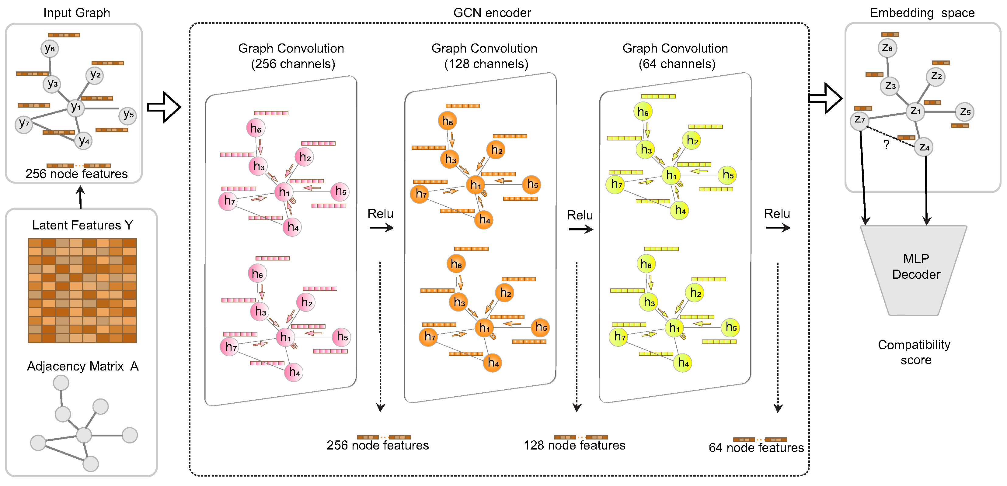
The GCN is a specialized architecture that excels at processing graph-based data structures. It is a mathematical transformer that converts information from its original domain to an embedding space. The GCN employs a sequence of graph convolution layers, as demonstrated in Figure 2, to gradually convert the initial node features into more abstract, low-dimensional embeddings suitable for downstream tasks. This transformation is accomplished by applying successive graph convolution operations that refine and condense the node features at each layer, as demonstrated by the transition from 256 node features to 64 node features in the architecture depicted. Applying a ReLU activation function to each layer improves the model’s capacity to detect intricate patterns in the data by introducing non-linearity.
GCNs, unlike traditional CNNs, excel in handling irregular, non-Euclidean graph structures. This capability addresses CNN’s limitations in graph applications and integrates innovative solutions within the graph processing domain. Kipf et al. [41] designed a semi-supervised graph convolution model with multi-layer propagation, significantly impacting our GCN design.
Consider a graph G = ( V , E ) , where A is the adjacency matrix that details the complex relationships between nodes, and D is the degree matrix. Each element D i j aggregates the connections in the i-th row of A. The GCN performs its primary convolution operation as follows [41,46]:  
H ( l + 1 ) = ReLU D ˜ 1 / 2 A ˜ D ˜ 1 / 2 H ( l ) W ( l )
where A ˜ = A + I incorporates self-connections by adding the identity matrix I, W ( l ) denotes the weight matrix for the l-th layer, σ represents a non-linear activation function such as ReLU, and H ( l ) are the activations at the l-th layer, beginning with H ( 0 ) = Y , the matrix of node features.
Despite its effectiveness, the standard GCN model faces challenges in handling diverse node and link types, which can limit its utility in detailed assessments of node interactions and compatibility predictions.
Our refined approach extends the GCN framework to accommodate a wider array of nodes and links. We redefine the graph G = ( V , E ) to encompass entities such as products and relational links, including ‘also viewed’ and ‘purchased together’. Each node is characterized by a feature vector x 1 , x 2 , , x N , which is transformed into y 1 , y 2 , , y N R d , where d represents the dimensionality.
The GCN encoder begins processing with latent feature vectors y i extracted via an autoencoder, capturing essential attributes like shape, color, and size. CNNs initially derive these features, and a stacked denoising autoencoder refines them to produce a condensed, low-dimensional representation.
The encoder then incorporates these refined features with data from nearby nodes, accomplishing this by [41]:
N i = { j V | A i j = 1 }
The GCN functions as an aggregator of local neighborhood information, symbolized by h ˜ i = f enc ( y ˜ i , N i ) , and maps data from R F to R F . This aggregation, facilitated by a deep GCN with several hidden layers, results in [46]:
H ( l + 1 ) = ReLU s = 0 S D ˜ s 1 / 2 A ˜ D ˜ s 1 / 2 H ( l ) W s ( l )
where l ranges from 0 to l 1 , and H ( 0 ) = Y . The matrix D ˜ s is diagonal, with its elements d i = j = 1 n A i j , and each convolution layer possesses a specific weight matrix W l sized R d k × d k + 1 . The parameter s sets the neighborhood scope during training, with S = 1 typically focusing on immediate neighbors. The weights W s ( l ) , located in R F × F , are enhanced through techniques like batch normalization, dropout, and weight regularization, optimizing the network’s performance.

3.3. Edge Prediction Layer

The Edge Prediction Layer is crucial for deducing probable edges or relationships between nodes after the GCN encoder has processed them. This layer employs the MLPDecoder architecture within our VAGCN model, similar to Garcia and Bruna’s work [47]. Primarily functioning as a multi-layer perceptron (MLP), this layer analyzes the embeddings of node pairs to determine the existence and strength of edges between them.
Given two nodes, i and j, the probability of an edge or compatibility between them is computed using the following formula:
p i j = σ ( z i z j w T + b )
where z i ( L ) and z j ( L ) represent the embeddings of nodes i and j at the L-th layer of the GCN, respectively. The vector w is a learnable weight, and b is a bias term, with σ ( · ) being the sigmoid activation function that normalizes the output to the range [0, 1].
This prediction mechanism culminates in a matrix P, where each element P i j denotes the predicted probability of a connection between nodes i and j. This matrix provides a detailed view of the potential relationships across the graph, reflecting the sophisticated learning achieved through the node embeddings.
Algorithm 1 illustrates the procedural steps employed by our model to assess compatibility scores between fashion items by effectively utilizing visual features and advanced graph-based analysis.
Algorithm 1 VAGCN Model for Predictive Compatibility Scoring
Require: 
Visual features of images X, Adjacency matrix A
Ensure: 
Compatibility score matrix P between items
 1:
Initialization:
 2:
Set L = 3                          ▹ Number of GCN layers
 3:
Set S = 1                          ▹ Neighbourhood context scope
 4:
for each fashion image do
 5:
     Extract CNN-F features, resulting in high-dimensional vector X
 6:
end for
 7:
Compress X to obtain latent feature representation Y
 8:
Obtain Z by executing Z = GCN _ ENCODER ( Y , A )                ▹ Embedding space
 9:
Obtain P of nodes i and j by executing P i j = EDGE _ PRED ( Z , i , j )
10:
Return compatibility score p
11:
function GCN_ENCODER( y , A )
12:
    Initialization:
13:
    Set A 0 to Identity matrix I
14:
    Set A 1 to I + A
15:
    Set initial feature vector H ( 0 ) to y
16:
    for each layer l from 0 to L 1  do
17:
        Compute H ( l + 1 ) as ReLU ( D ˜ 1 / 2 A ˜ D ˜ 1 / 2 H ( l ) W ( l ) )
18:
    end for
19:
    return  H ( L )
20:
end function
21:
function EDGE_PRED( Z , i , j )
22:
    Compute P i j as σ ( z i z j w T + b )
23:
    return  P i j
24:
end function

3.4. Computational Complexity

In this study, we implemented several strategies to improve the computational cost of compatibility prediction. Firstly, using a deep-stacked autoencoder, we significantly reduced the node representation feature set from 4096 to 256 as a preprocessing step. For a three-layer autoencoder, the time complexity can be calculated as O ( n · D · d ) , where D is the original feature dimension and d is the dimension of the hidden layers. Due to the precomputed features, this preprocessing step reduces the dimensionality of the input data, enabling faster computations in subsequent steps without increasing the computational burden of the real-time application.
The VAGCN model’s computational complexity for predictive compatibility scoring consists of several key steps. The algorithm utilizes three graph convolutional layers ( L = 3 ) and considers neighbors one step away ( S = 1 ). The core of the complexity lies in the GCN encoder function, which normalizes the adjacency matrix and performs the convolution operations. Specifically, the adjacency matrix normalization step, A ˜ = D ˜ 1 / 2 A D ˜ 1 / 2 , involves matrix multiplication with a complexity of O ( | E | · d ) , where | E | is the number of edges and d is the feature dimension. Each graph convolutional layer computes new node embeddings, with the primary operations being matrix multiplications of the form A ˜ H ( l ) W ( l ) , having a complexity of O ( N · d 2 ) per layer, where N is the number of nodes. Given that there are L layers, the total complexity for the convolution operations is O ( L · N · d 2 ) .
The Edge Prediction Layer computes the compatibility score by calculating the difference between node embeddings and applying a logistic function, which has a complexity of O ( d ) for each node pair. Therefore, the overall computation complexity for the algorithm is dominated by the graph convolutional operations, leading to a final complexity of O ( L · N · d 2 + | E | · d ) .
Additionally, integrating the visual features into the GCN added complexity as we needed to balance computational load with model accuracy. Instead of using a uniform 256 hidden units for each layer in the 3-layer GCN architecture, we adopted a more efficient architecture with decreasing hidden units: d ( 1 ) = 256 , d ( 2 ) = 128 , and d ( 3 ) = 64 . This design reduces the computational burden and improves performance and accuracy, as our comparative results show. Lastly, during training, we consider neighbors only one step away ( S = 1 ) instead of a larger number of neighbors, which minimizes the number of operations. However, during testing, we consider a larger number of neighbors to ensure a thorough evaluation, which increases the computational complexity to O ( L · N · s L · d 2 ) . This increase in complexity is necessary for making more accurate predictions during testing while the training process remains efficient. These optimizations collectively address the technical challenges and enhance the algorithm’s efficiency while maintaining or even improving predictive performance.

4. Experimental Implementation

We evaluate the VAGCN model across various datasets, providing a comparative analysis against established baselines and examining key performance indicators. The intent is to comprehensively understand the model’s operational efficacy and transformative potential in fashion-oriented e-commerce platforms.

4.1. Dataset

We utilize the Amazon products dataset, which encompasses over 180 million product relationships spanning nearly six million distinct items, primarily in the fashion sector [23,24]. This dataset provides a robust framework for analyzing compatibility across various fashion segments, including men’s, women’s, and children’s apparel. We classify product interactions into three categories: also_viewed, bought_together, and also_bought, assuming that products purchased or added to the cart together are compatible. The analytical results are summarized in Table 2, which details the intricate interaction dynamics within this dataset.

4.2. Feature Extraction and Graph Construction

The visual features for fashion items, extracted using a CNN pretrained on the ImageNet dataset, capture complex attributes such as shapes, colors, and textures. These features are subsequently condensed via an autoencoder, forming the basis for our graph construction, where nodes represent products and edges reflect compatibility relationships. To enhance the model’s training process, we construct a training set comprising both positive edges and negative edges. Positive edges are directly extracted from the existing connections in the adjacency matrix A, representing compatible product pairs. Conversely, we randomly generate negative samples by selecting an equal number of non-relationships that do not exist as edges in the adjacency matrix. These non-relationships represent product pairs that have not been viewed or bought together, providing a clear contrast to the positive pairs and helping the model effectively learn to distinguish between compatible and incompatible items. This methodology ensures a comprehensive learning scenario, facilitating the model’s robust performance in predicting product compatibility.

4.3. Model Training

Training of the VAGCN begins with the autoencoder component. We initialize the model with normalized input vectors corresponding to the feature dimensions of the dataset. This autoencoder progresses through several dense layers, ultimately reducing the feature space to a 256-dimensional hidden layer that captures essential characteristics of fashion images. Optimization is carried out using stochastic gradient descent (SGD) with a learning rate of 0.1 and momentum of 0.9. ReLU activation is employed across all layers to preserve non-linear processing capabilities. The training aims to minimize the mean squared error across 100 epochs with a batch size of 256 to refine the network for accurate feature extraction tailored to fashion item compatibility [22].
Subsequently, the model trains a GCN using the encoded 256-dimensional vectors. The GCN is structured into layers with (256, 128, 64) hidden units each [48]. During this phase, the learning rate is adjusted to 0.01, with no weight decay implemented to preserve delicate feature representations. A dropout rate of 0.5 [49] and batch normalization are applied to ensure generalization and training stability [50]. Over 300 epochs, the GCN learns to discern intricate relationships between fashion items, enhancing product compatibility prediction accuracy. The data split used for training, validation, and testing follows the proportions of 80%, 10%, and 10%, respectively, as outlined in [24], to ensure a fair comparison with established methodologies.

4.4. Baseline Models

To properly evaluate the model, it is important to benchmark its performance against classical approaches. We evaluate our model with the baseline methods offered by McAuley et al. [24]:
  • Category Tree (CT): This method directly utilizes Amazon’s intricate category tree, exploiting the structured hierarchies inherent in the platform’s product categories. The CT approach acts as a benchmark to gauge the upper-performance limit of an image-based classification model, particularly in its ability to discern category-specific distinctions.
  • Weighted Nearest Neighbor (WNN): The WNN method applies a classification paradigm that utilizes weighted distances between data points. This approach emphasizes the importance of each neighbor’s contribution to the classification decision, enhancing prediction accuracy.
  • Compatibility Metric on CNN-Extracted Features (McAuley et al.): This technique, originally described by McAuley et al. [24], focuses on visual compatibility prediction. It is based on a compatibility metric that utilizes features extracted from CNNs. This metric, reliant on the distance within the feature embedding space, offers insights into the compatibility between product pairs.
Employing these baselines allows us to critically assess the relative performance of our proposed model, with a specific focus on its efficiency and reliability in a real-world application scenario.

4.5. Model Evaluation Matrices

The performance of the VAGCN model is rigorously evaluated using a comprehensive suite of metrics designed to reflect both accuracy and practical applicability in real-world e-commerce scenarios. Detailed evaluations include:
  • Loss Analysis: To track the model’s performance during training and validation, we use a cross-entropy loss function, as defined in [51]. The loss function is expressed as:
    L ( y , y ^ ) = 1 N i = 1 N [ y i log ( σ ( y ^ i ) ) ( 1 y i ) log ( 1 σ ( y ^ i ) ) ]
    where y i represents the actual label, and y ^ i is the predicted value before applying the sigmoid function, σ ( y ^ i ) = 1 1 + e y ^ i , which converts it into a probability. The first term, y i log ( σ ( y ^ i ) ) , penalizes the model when the true label is 1, and the prediction is incorrect (i.e., y ^ i is close to 0). The second term, ( 1 y i ) log ( 1 σ ( y ^ i ) ) , penalizes the model when the true label is 0, and the prediction incorrectly suggests a positive outcome (i.e., y ^ i is close to 1). By summing these penalties across all N samples, the function provides a measure of how well the model’s predictions match the actual labels. This balanced approach ensures the model learns effectively, helping prevent overfitting and improving its ability to generalize to new data.
  • Accuracy Measurement: Accuracy metrics quantify the model’s ability to align predictions with actual labels. This is calculated as:
    Accuracy = 1 N i = 1 N 1 ( round ( σ ( y ^ i ) ) = y i )
    where the round function maps the sigmoid output to the nearest integer.
  • Area under the ROC Curve (AUC) Evaluation: We compute the area under the Receiver Operating Characteristic Curve (AUC-ROC) to assess the model’s ability to distinguish between compatible and incompatible item pairs, which is indicative of model performance [52]. The AUC is calculated as:
    AUC = 0 1 TPR ( t ) d FPR ( t )
    where t is the threshold for classifying predicted probabilities as positive or negative.
  • Neighborhood-Based Evaluation: In the fashion industry, understanding outfit compatibility extends beyond analyzing individual items. Insights from neighboring nodes can provide a comprehensive view, particularly when integrating the visual attributes of multiple nodes. In our model, the k-neighborhood of a node i in the relational graph is defined by the set of k nodes accessible through a layered traversal method akin to ‘breadth-first-search’. During the testing phase, each dataset encompasses the primary items and their associated K-neighborhoods. This allows for systematically evaluating our model’s performance as the value of k is varied. For k = 1 , the model focuses on the features directly linked to the outfit’s node. However, as k increases, the item embeddings begin to utilize knowledge from a wider array of neighboring nodes. This expanded neighborhood evaluation method is employed explicitly during the testing phase. Detailed results for varying k values are presented in subsequent sections.

5. Results & Discussion

5.1. VAGCN Performance and Comparisons

In our comprehensive evaluation, we compared the performance of the VAGCN model to baseline methods using several key e-commerce interaction metrics, including also_viewed, also_bought, and bought_together. This comparative analysis was conducted across diverse product categories: men, women, boys, girls, and babies. Our results, as detailed in Table 3, show that the VAGCN model not only meets but consistently exceeds the performance of established benchmarks like the Category Tree (CT), Weighted Nearest Neighbor (WNN), and the methodologies developed by McAuley et al. For instance, in the men’s category, the VAGCN achieves an accuracy of 97.1%, notably surpassing the 91.6% recorded by McAuley et al., which amounts to a substantial improvement of 5.5%. This advancement underscores VAGCN’s superior capability in integrating complex visual data into the graph-based learning framework, which is essential for accurately predicting visual compatibility in fashion items.
Similarly, the VAGCN model also excels in the also_bought and bought_together interactions, demonstrating its robustness across different types of e-commerce interactions. For the also_bought interaction in the women’s segment, VAGCN records an accuracy of 93.9%, a significant gain of 6.1 percentage points over McAuley et al.’s 87.8%. In the Boys category, VAGCN further illustrates its effectiveness with an accuracy of 96.0% for the same interaction type, outperforming McAuley et al.’s 94.1%. These results highlight VAGCN’s ability to capture and utilize complex relational and visual data effectively, facilitating precise compatibility predictions across a broad spectrum of products. This performance not only showcases the technical strengths of the VAGCN framework but also its practical utility in enhancing recommendation accuracy in the dynamic environment of fashion e-commerce.
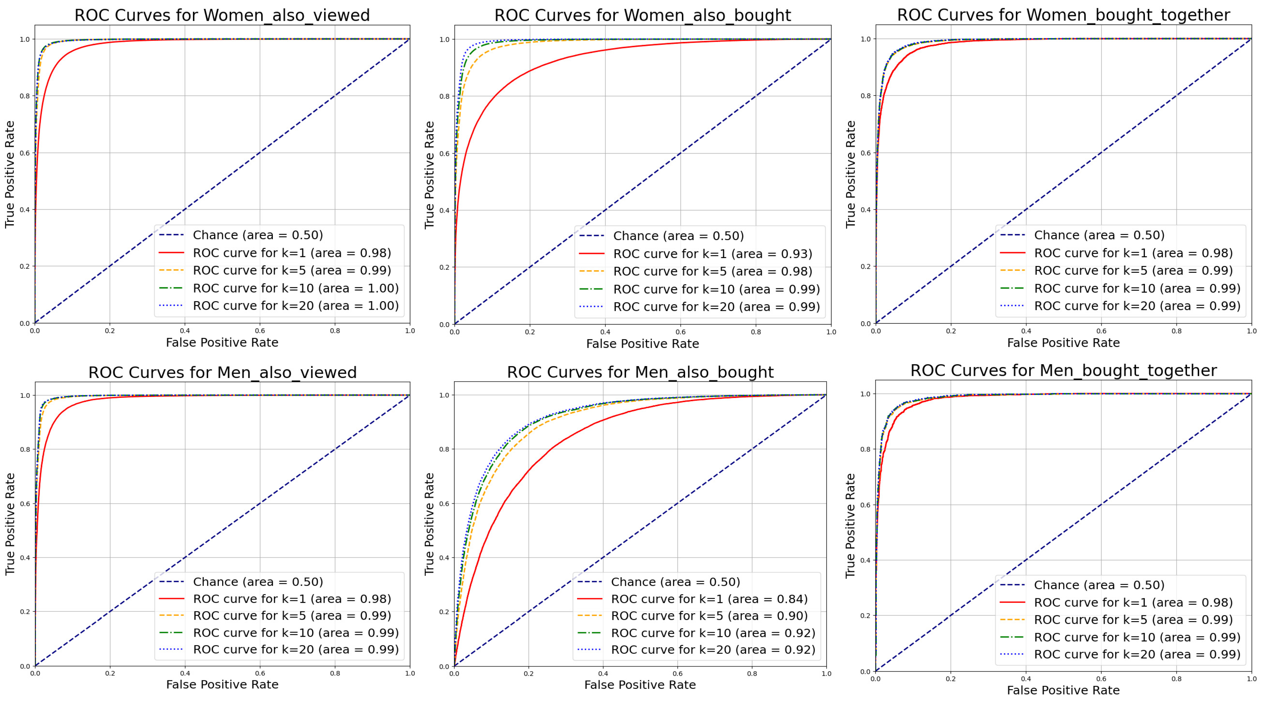
Furthermore, the Receiver Operating Characteristic (ROC) curves for the women’s and men’s category interactions illustrate the model’s robust performance across different k values (see Figure 3). For the women’s category, the area under the curve (AUC) for also_viewed interactions improves from 0.98 at k = 1 to a perfect 1.00 at k = 10 , indicating near-perfect classifier performance at higher neighborhood settings. Similarly, for the men’s category, the AUC for also_viewed interactions begins at 0.98 at k = 1 and reaches 0.99 by k = 10 . Comparable trends are observed in the AUC values for also_bought and bought_together interactions across both categories, where the AUC values reach or closely approach 1.00, underscoring the exceptional discriminatory ability of the model to accurately classify compatible and incompatible item pairs with minimal false positive rates.

5.2. Loss Analysis

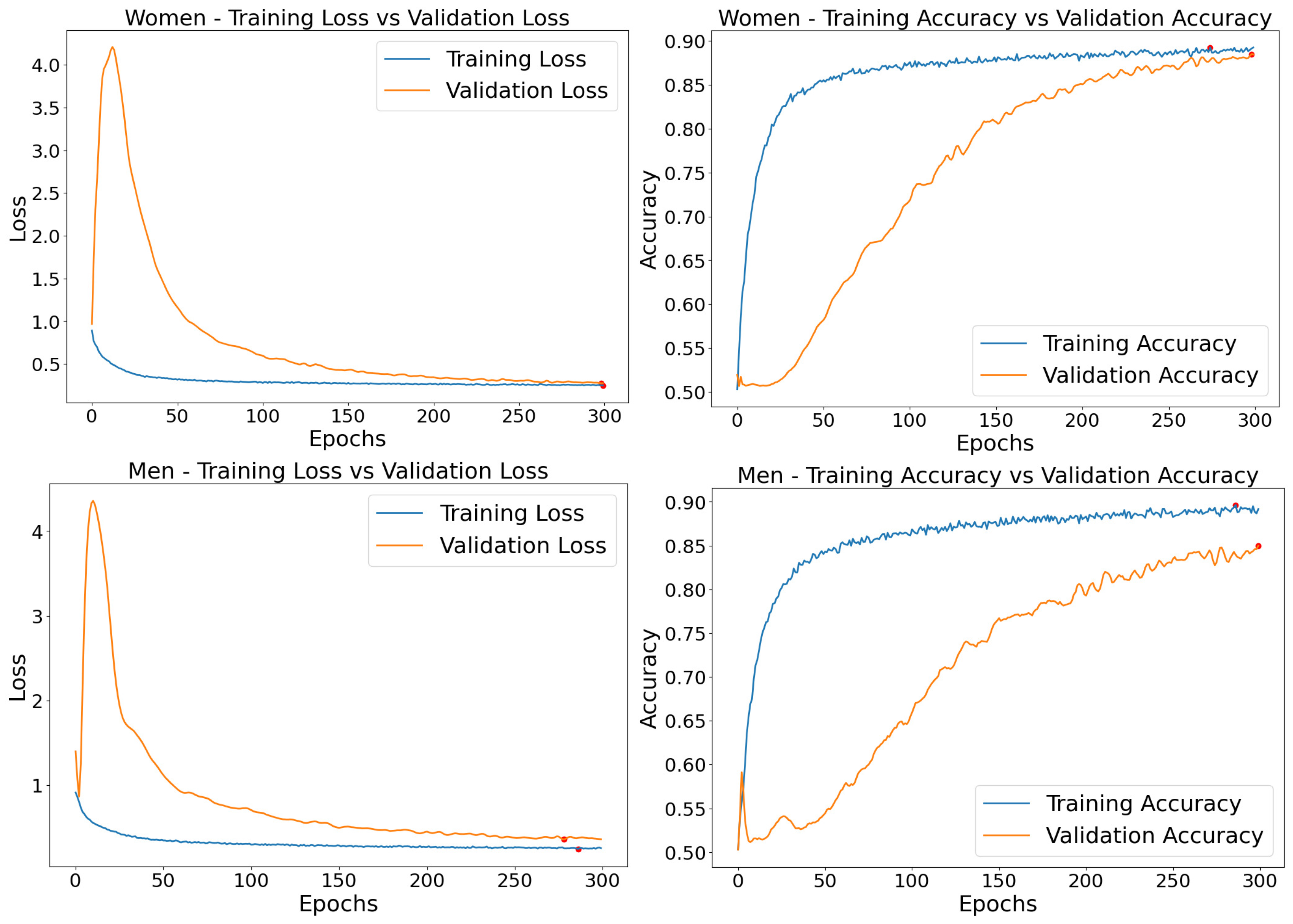
The evaluation of performance metrics obtained from our training sessions with the VAGCN underscores its efficacy, especially when applied to the women’s and men’s datasets. As depicted in Figure 4, the training loss has a tendency towards approaching zero, which indicates the model’s high level of accuracy in accurately fitting the dataset. The validation loss exhibits a consistent decrease and then reaches a stable point at a low level, highlighting the model’s capacity to effectively adapt to new data, which is essential for practical implementation.
In addition, the accuracy metrics observed during these sessions were highly promising. Training accuracy consistently increased, peaking at around 95%, while the validation accuracy recorded significant gains, reaching up to 85% (see Figure 4). These measures demonstrate that the model is accurately capturing the patterns in the dataset without overfitting. The model’s durability and capability to generate accurate predictions are highlighted by its ability to achieve high accuracy and low loss during both the training and validation phases.

5.3. Impact of Neighborhood Size

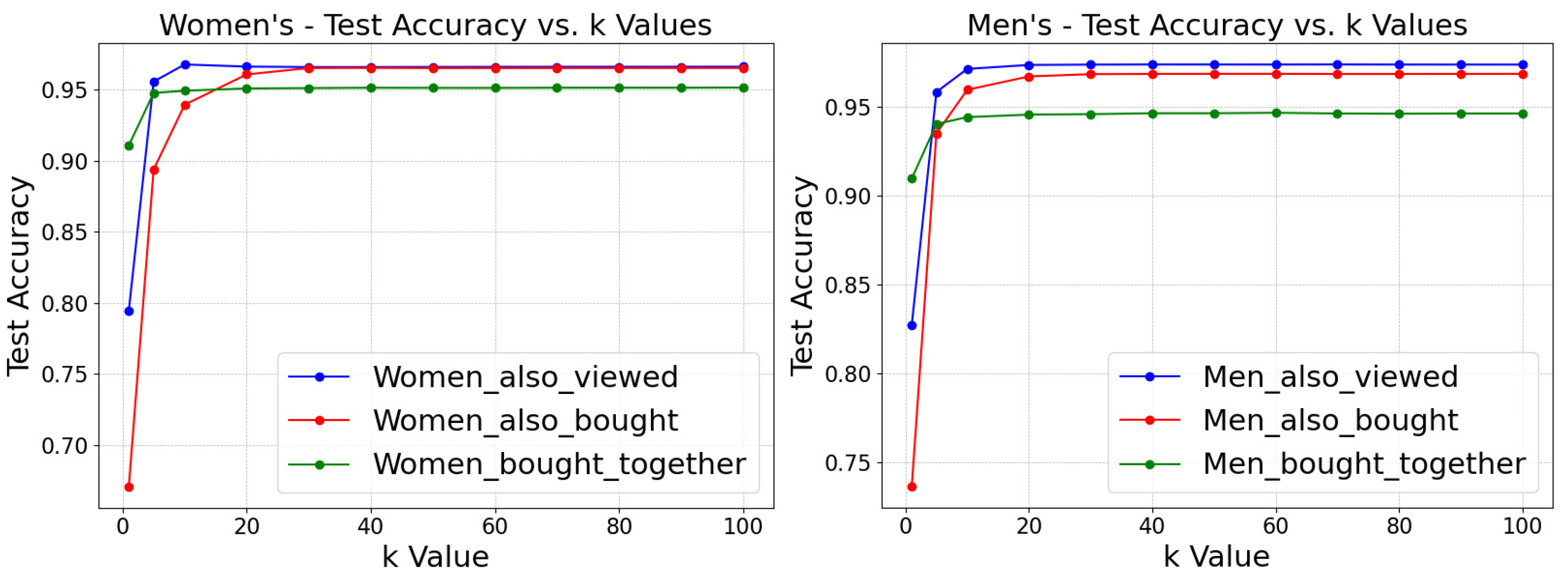
Evaluating the VAGCN across varying neighborhood sizes (k-values) provided significant insights into its performance, specifically regarding its predictive capabilities in the men’s and women’s categories. The results, as depicted in Figure 5, reveal a marked improvement in test accuracy as the neighborhood size increases from k = 1 to k = 20. After reaching this stage, the accuracy stabilizes, remaining at approximately 95% for both categories. This observation suggests an optimal k-value threshold, beyond which additional neighboring nodes contribute minimally to further accuracy gains, thus highlighting an efficiency frontier for computational resources versus predictive performance.
This analysis validates the effectiveness of a neighborhood-based evaluation strategy, where extending the node context to an optimal point significantly enhances the model’s predictive accuracy. It is essential to determine the best k-value for refining the VAGCN model in real applications. This will ensure that contextual data is used optimally for correct compatibility assessments while avoiding unnecessary computing costs.

5.4. Parameter Evaluations

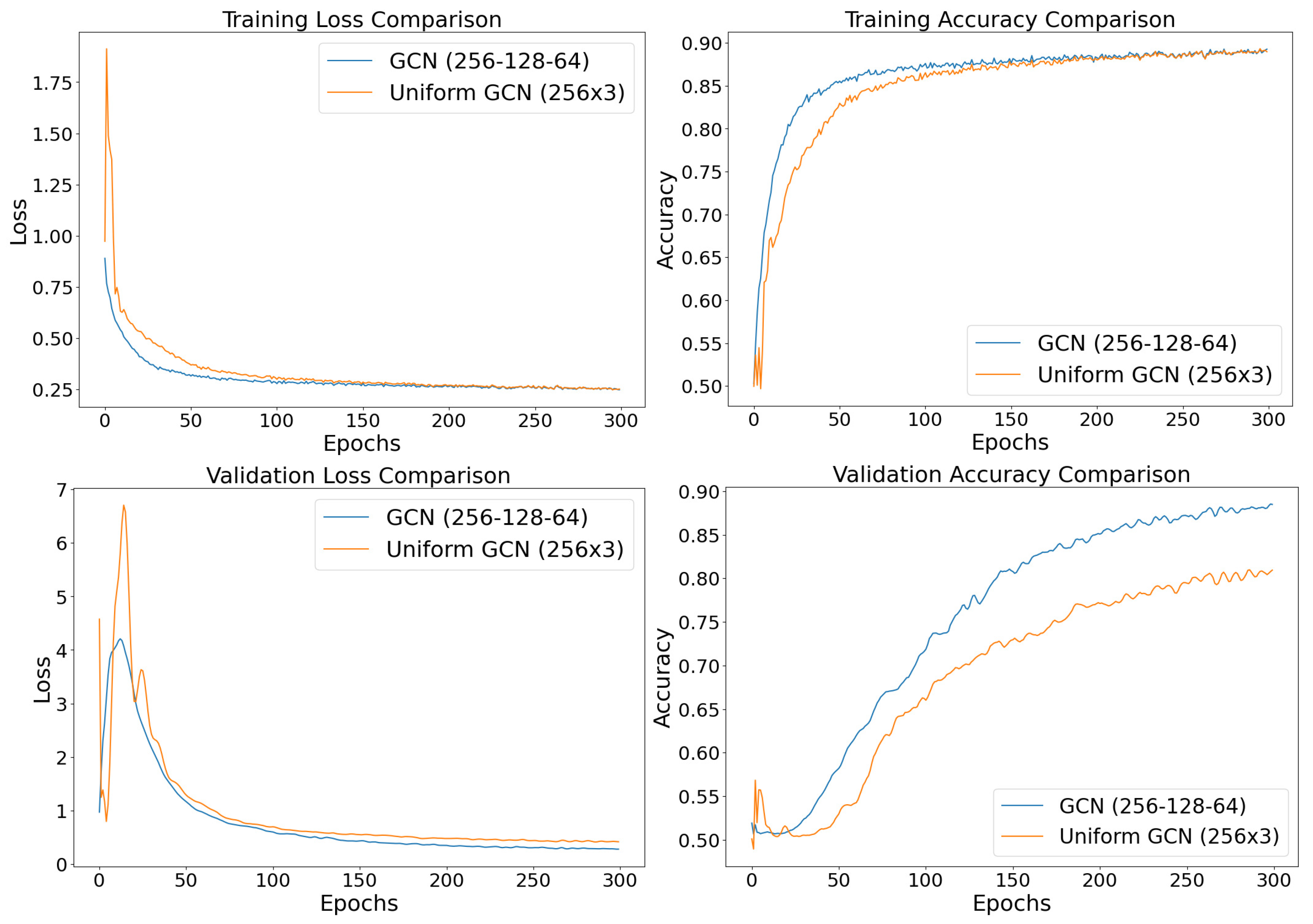
Our performance analysis of two distinct GCN configurations, illustrated through training loss and accuracy plots in Figure 6, reveals significant differences. The GCN with decreasing layer sizes (256, 128, 64) demonstrates a more stable reduction in training loss from the outset, avoiding the initial spikes in loss observed in the uniform GCN configuration (256 × 3). This stability is essential for consistent learning across epochs. The architecture, which decreases the number of features from 256 to 64 in each layer, effectively combines features from nearby nodes. This configuration aligns with insights from the VAGCN study, highlighting the benefits of careful feature scaling and neighborhood sizing in enhancing model performance while minimizing computational overhead.
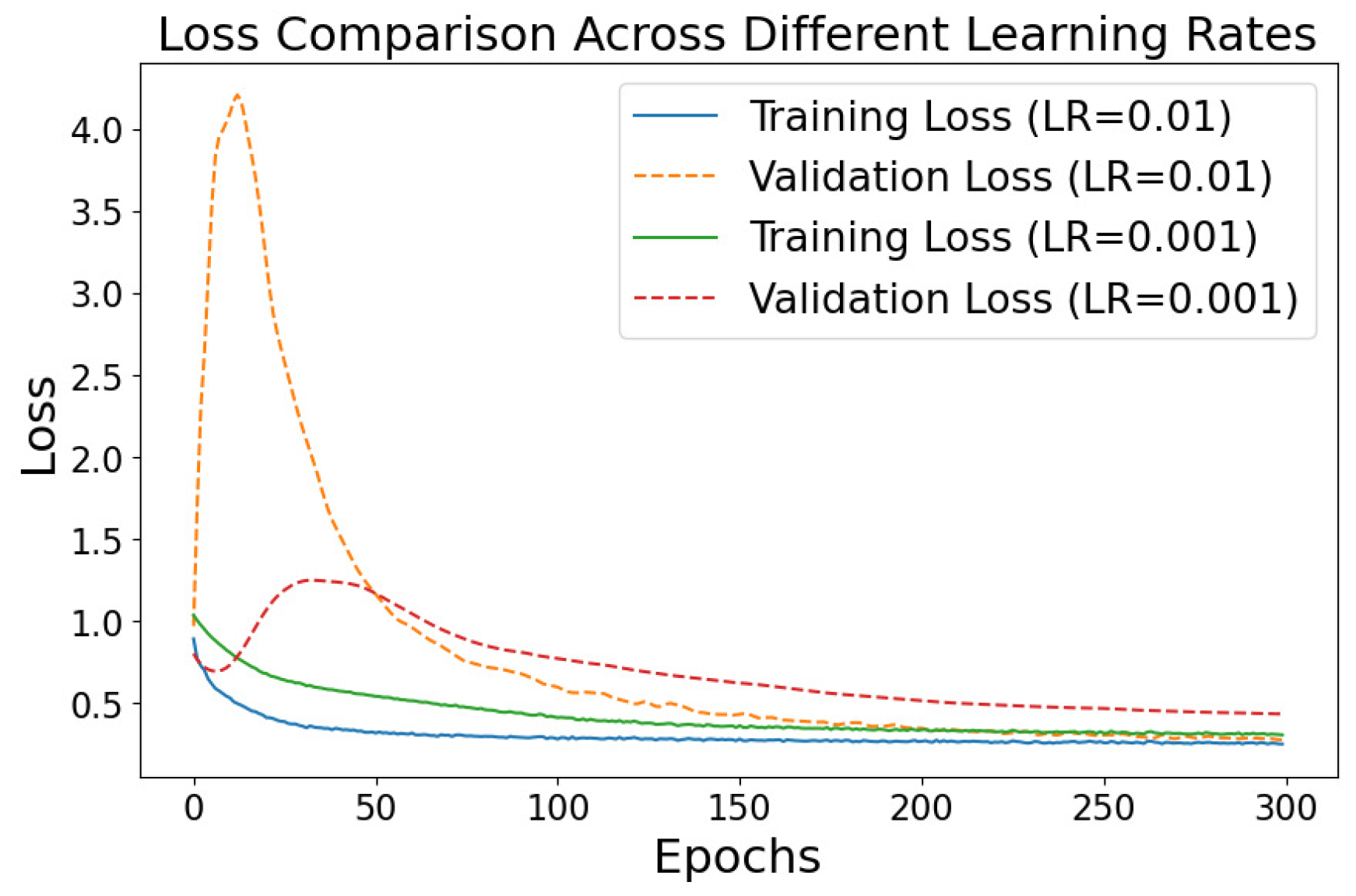
Further parameter evaluation focused on learning rates, which demonstrated a significant advantage when using a rate of 0.01. As shown in Figure 7, this learning rate effectively and quickly reduces loss, stabilizing at an optimal level that leads to the highest accuracies observed across all tested datasets. After an initial rapid decline, the rate stabilizes, ensuring consistent and excellent performance while avoiding the overfitting of the model. This finding indicates that a higher learning rate effectively navigates the model’s complex loss surface, efficiently locating optimal solutions. Consequently, a learning rate of 0.01 accelerates the initial phases of model training and improves long-term generalization capabilities.

5.5. Visualization of Compatibility Score

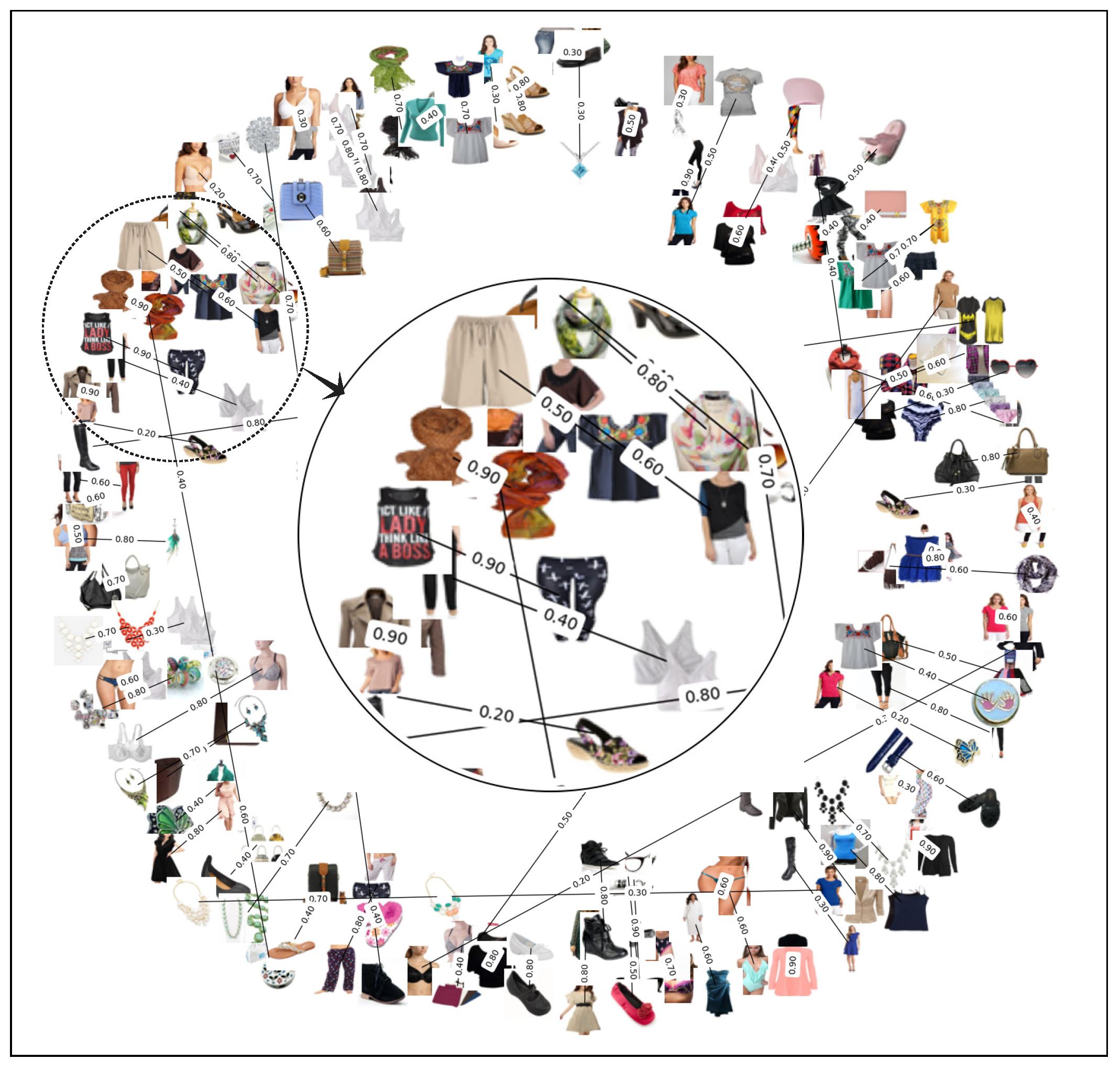
In our study, we employ graph visualization to analyze the link prediction task on a dataset composed of women’s fashion items, as shown in Figure 8; visual representation serves as a powerful tool to discern how different items are predicted to be compatible or incompatible based on their visual attributes. In the graph, each edge connects a pair of items, with the edge weight reflecting the predicted compatibility score. This methodological approach facilitates the identification of potential patterns and relationships within the dataset, thereby offering insights into how various attributes—such as color, style, and texture—play a role in compatibility predictions.
This visualization underscores the model’s ability to identify and quantify aesthetic relationships between diverse fashion items and enhances our understanding of the elements contributing to successful outfit combinations. Through this analysis, we can better appreciate how the model leverages visual attributes to facilitate robust and intuitive compatibility assessments.

6. Conclusions

In conclusion, our model has demonstrated its importance as a key innovation in fashion e-commerce by addressing the complex challenge of predicting item compatibility through visual feature analysis. The VAGCN framework has successfully converted high-dimensional CNN features into actionable insights by utilizing GCN with deep-stacked autoencoders, thereby improving the precision of compatibility predictions across various fashion categories. However, while the VAGCN model demonstrates significant improvements, it has certain limitations. Specifically, it may face challenges in extremely sparse or cold-start scenarios where relational data is limited. Additionally, the compression of high-dimensional visual features could result in the loss of fine-grained details, potentially affecting recommendation accuracy in some cases.
Looking forward, we see immense potential in combining GCNs with advanced techniques in representation learning or feature transformation, which can further refine the model’s ability to capture and utilize high-dimensional visual data. Future work could also focus on integrating multi-modal learning or incorporating textual descriptions alongside visual features to enrich item representations. This combination could lead to more personalized and visually cohesive recommendations, paving the way for the next generation of intelligent, visually aware recommendation systems.

Author Contributions

U.S.M. conducted the primary experiments, performed evaluations, and drafted the initial manuscript. J.Z., the corresponding author, supervised the project and provided strategic oversight, specifically focusing on the innovation aspects of the paper. A.R. and S.S. contributed to the experimental analysis and manuscript refinement. All authors have read and agreed to the published version of the manuscript.

Funding

This work was partly supported by grants from the Natural Science Foundation of China (Nos.: 62372101, 61873337, 62272097).

Data Availability Statement

The datasets can be accessed through the following link: https://jmcauley.ucsd.edu/data/amazon/ (accessed on 8 August 2024). The implementation for VAGCN is available at https://github.com/umarsubhanmalhi/VA_GCN/ (accessed on 8 August 2024).

Conflicts of Interest

The authors declare no conflicts of interest.

References

  1. Chen, H.J.; Shuai, H.H.; Cheng, W.H. A survey of artificial intelligence in fashion. IEEE Signal Process. Mag. 2023, 40, 64–73. [Google Scholar] [CrossRef]
  2. Hidayati, S.C.; Goh, T.W.; Chan, J.S.G.; Hsu, C.C.; See, J.; Wong, L.K.; Hua, K.L.; Tsao, Y.; Cheng, W.H. Dress with style: Learning style from joint deep embedding of clothing styles and body shapes. IEEE Trans. Multimed. 2020, 23, 365–377. [Google Scholar] [CrossRef]
  3. Ding, Y.; Lai, Z.; Mok, P.; Chua, T.S. Computational Technologies for Fashion Recommendation: A Survey. ACM Comput. Surv. 2023, 56, 121. [Google Scholar] [CrossRef]
  4. Zanker, M.; Rook, L.; Jannach, D. Measuring the impact of online personalisation: Past, present and future. Int. J. Hum.-Comput. Stud. 2019, 131, 160–168. [Google Scholar] [CrossRef]
  5. Markchom, T.; Liang, H.; Ferryman, J. Scalable and explainable visually-aware recommender systems. Knowl.-Based Syst. 2023, 263, 110258. [Google Scholar] [CrossRef]
  6. Gao, C.; Zheng, Y.; Li, N.; Li, Y.; Qin, Y.; Piao, J.; Quan, Y.; Chang, J.; Jin, D.; He, X.; et al. A survey of graph neural networks for recommender systems: Challenges, methods, and directions. ACM Trans. Recomm. Syst. 2023, 1, 3. [Google Scholar] [CrossRef]
  7. Wang, L.; Guo, D.; Liu, X. Research on Intelligent Recommendation Technology for Complex Tasks. In Proceedings of the 2023 4th IEEE International Conference on Computer Engineering and Application (ICCEA), Hangzhou, China, 7–9 April 2023; pp. 353–360. [Google Scholar]
  8. Dossena, M.; Irwin, C.; Portinale, L. Graph-based recommendation using graph neural networks. In Proceedings of the 2022 21st IEEE International Conference on Machine Learning and Applications (ICMLA), Nassau, Bahamas, 12–14 December 2022; pp. 1769–1774. [Google Scholar]
  9. Zzh; Zhang, W.; Wentao. Industrial Solution in Fashion-Domain Recommendation by an Efficient Pipeline Using GNN and Lightgbm. In Proceedings of the Recommender Systems Challenge, Seattle, WA, USA, 18–23 September 2022; pp. 45–49. [Google Scholar]
  10. Vasileva, M.I.; Plummer, B.A.; Dusad, K.; Rajpal, S.; Kumar, R.; Forsyth, D. Learning type-aware embeddings for fashion compatibility. In Proceedings of the European Conference on Computer Vision (ECCV), Munich, Germany, 8–14 September 2018; pp. 390–405. [Google Scholar]
  11. Kuang, Z.; Gao, Y.; Li, G.; Luo, P.; Chen, Y.; Lin, L.; Zhang, W. Fashion retrieval via graph reasoning networks on a similarity pyramid. In Proceedings of the IEEE/CVF International Conference on Computer Vision, Seoul, Republic of Korea, 27 October–2 November 2019; pp. 3066–3075. [Google Scholar]
  12. Marcuzzo, M.; Zangari, A.; Albarelli, A.; Gasparetto, A. Recommendation systems: An insight into current development and future research challenges. IEEE Access 2022, 10, 86578–86623. [Google Scholar] [CrossRef]
  13. Ferreira, D.; Silva, S.; Abelha, A.; Machado, J. Recommendation system using autoencoders. Appl. Sci. 2020, 10, 5510. [Google Scholar] [CrossRef]
  14. Xie, Y.; Yao, C.; Gong, M.; Chen, C.; Qin, A.K. Graph convolutional networks with multi-level coarsening for graph classification. Knowl.-Based Syst. 2020, 194, 105578. [Google Scholar] [CrossRef]
  15. Papadakis, H.; Papagrigoriou, A.; Panagiotakis, C.; Kosmas, E.; Fragopoulou, P. Collaborative filtering recommender systems taxonomy. Knowl. Inf. Syst. 2022, 64, 35–74. [Google Scholar] [CrossRef]
  16. Cai, H.; Zheng, V.W.; Chang, K.C.C. A comprehensive survey of graph embedding: Problems, techniques, and applications. IEEE Trans. Knowl. Data Eng. 2018, 30, 1616–1637. [Google Scholar] [CrossRef]
  17. Georgiou, T.; Liu, Y.; Chen, W.; Lew, M. A survey of traditional and deep learning-based feature descriptors for high dimensional data in computer vision. Int. J. Multimed. Inf. Retr. 2020, 9, 135–170. [Google Scholar] [CrossRef]
  18. Jing, L.; Vincent, P.; LeCun, Y.; Tian, Y. Understanding dimensional collapse in contrastive self-supervised learning. In Proceedings of the 10th International Conference on Learning Representations, ICLR 2022, Virtual, 25–29 April 2022. [Google Scholar]
  19. Tao, Y.; Guo, K.; Zheng, Y.; Pan, S.; Cao, X.; Chang, Y. Breaking the curse of dimensional collapse in graph contrastive learning: A whitening perspective. Inf. Sci. 2024, 657, 119952. [Google Scholar] [CrossRef]
  20. Tran, B.; Tran, D.; Nguyen, H.; Ro, S.; Nguyen, T. scCAN: Single-cell clustering using autoencoder and network fusion. Sci. Rep. 2022, 12, 10267. [Google Scholar] [CrossRef] [PubMed]
  21. Yan, C.; Malhi, U.S.; Huang, Y.; Tao, R. Unsupervised deep clustering for fashion images. In Proceedings of the Knowledge Management in Organizations: 14th International Conference, KMO 2019, Zamora, Spain, 15–18 July 2019; Proceedings 14. Springer: Berlin/Heidelberg, Germany, 2019; pp. 85–96. [Google Scholar]
  22. Malhi, U.S.; Zhou, J.; Yan, C.; Rasool, A.; Siddeeq, S.; Du, M. Unsupervised Deep Embedded Clustering for High-Dimensional Visual Features of Fashion Images. Appl. Sci. 2023, 13, 2828. [Google Scholar] [CrossRef]
  23. He, R.; McAuley, J. Ups and downs: Modeling the visual evolution of fashion trends with one-class collaborative filtering. In Proceedings of the 25th International Conference on World Wide Web, Montreal, QC, Canada, 11–15 April 2016; pp. 507–517. [Google Scholar]
  24. McAuley, J.; Targett, C.; Shi, Q.; Van Den Hengel, A. Image-based recommendations on styles and substitutes. In Proceedings of the 38th International ACM SIGIR Conference on Research and Development in Information Retrieval, Santiago, Chile, 9–13 August 2015; pp. 43–52. [Google Scholar]
  25. Sarkar, R.; Bodla, N.; Vasileva, M.; Lin, Y.L.; Beniwal, A.; Lu, A.; Medioni, G. Outfittransformer: Outfit representations for fashion recommendation. In Proceedings of the IEEE/CVF Conference on Computer Vision and Pattern Recognition, New Orleans, LA, USA, 18–24 June 2022; pp. 2263–2267. [Google Scholar]
  26. Deldjoo, Y.; Nazary, F.; Ramisa, A.; Mcauley, J.; Pellegrini, G.; Bellogin, A.; Noia, T.D. A review of modern fashion recommender systems. ACM Comput. Surv. 2023, 56, 1–37. [Google Scholar] [CrossRef]
  27. Cardoso, Â.; Daolio, F.; Vargas, S. Product characterisation towards personalisation: Learning attributes from unstructured data to recommend fashion products. In Proceedings of the 24th ACM SIGKDD International Conference on Knowledge Discovery & Data Mining, London, UK, 19–23 August 2018; pp. 80–89. [Google Scholar]
  28. Hong, W.; Li, S.; Hu, Z.; Rasool, A.; Jiang, Q.; Weng, Y. Improving relation extraction by knowledge representation learning. In Proceedings of the 2021 IEEE 33rd International Conference on Tools with Artificial Intelligence (ICTAI), Washington, DC, USA, 1–3 November 2021; pp. 1211–1215. [Google Scholar]
  29. Jagadeesh, V.; Piramuthu, R.; Bhardwaj, A.; Di, W.; Sundaresan, N. Large scale visual recommendations from street fashion images. In Proceedings of the 20th ACM SIGKDD International Conference on Knowledge Discovery and Data Mining, New York, NY, USA, 24–27 August 2014; pp. 1925–1934. [Google Scholar]
  30. Deldjoo, Y.; Di Noia, T.; Malitesta, D.; Merra, F.A. A study on the relative importance of convolutional neural networks in visually-aware recommender systems. In Proceedings of the IEEE/CVF Conference on Computer Vision and Pattern Recognition, Nashville, TN, USA, 20–25 June 2021; pp. 3961–3967. [Google Scholar]
  31. He, R.; McAuley, J. VBPR: Visual bayesian personalized ranking from implicit feedback. In Proceedings of the AAAI Conference on Artificial Intelligence, Phoenix, AZ, USA, 12–17 February 2016; Volume 30. [Google Scholar]
  32. Liu, Q.; Wu, S.; Wang, L. Deepstyle: Learning user preferences for visual recommendation. In Proceedings of the 40th International Acm Sigir Conference on Research and Development in Information Retrieval, Shinjuku, Japan, 7–11 August 2017; pp. 841–844. [Google Scholar]
  33. Yan, C.; Chen, Y.; Zhou, L. Differentiated fashion recommendation using knowledge graph and data augmentation. IEEE Access 2019, 7, 102239–102248. [Google Scholar] [CrossRef]
  34. Yu, W.; He, X.; Pei, J.; Chen, X.; Xiong, L.; Liu, J.; Qin, Z. Visually aware recommendation with aesthetic features. VLDB J. 2021, 30, 495–513. [Google Scholar] [CrossRef]
  35. Dong, M.; Zeng, X.; Koehl, L.; Zhang, J. An interactive knowledge-based recommender system for fashion product design in the big data environment. Inf. Sci. 2020, 540, 469–488. [Google Scholar] [CrossRef]
  36. Li, Y.; Cao, L.; Zhu, J.; Luo, J. Mining fashion outfit composition using an end-to-end deep learning approach on set data. IEEE Trans. Multimed. 2017, 19, 1946–1955. [Google Scholar] [CrossRef]
  37. Liu, L.; Du, X.; Zhu, L.; Shen, F.; Huang, Z. Learning discrete hashing towards efficient fashion recommendation. Data Sci. Eng. 2018, 3, 307–322. [Google Scholar] [CrossRef]
  38. Cohen-Shapira, N.; Rokach, L. Learning dataset representation for automatic machine learning algorithm selection. Knowl. Inf. Syst. 2022, 64, 2599–2635. [Google Scholar] [CrossRef]
  39. Yi, J.; Chen, Z. Multi-modal variational graph auto-encoder for recommendation systems. IEEE Trans. Multimed. 2021, 24, 1067–1079. [Google Scholar] [CrossRef]
  40. Ma, M.; Na, S.; Wang, H. AEGCN: An autoencoder-constrained graph convolutional network. Neurocomputing 2021, 432, 21–31. [Google Scholar] [CrossRef]
  41. Kipf, T.N.; Welling, M. Variational Graph Auto-Encoders. arXiv 2016, arXiv:1611.07308. [Google Scholar]
  42. Veit, A.; Kovacs, B.; Bell, S.; McAuley, J.; Bala, K.; Belongie, S. Learning visual clothing style with heterogeneous dyadic co-occurrences. In Proceedings of the IEEE International Conference on Computer Vision, Santiago, Chile, 7–13 December 2015; pp. 4642–4650. [Google Scholar]
  43. Yin, R.; Li, K.; Lu, J.; Zhang, G. Enhancing fashion recommendation with visual compatibility relationship. In Proceedings of the World Wide Web Conference, San Francisco, CA, USA, 13–17 May 2019; pp. 3434–3440. [Google Scholar]
  44. Borges, R.; Stefanidis, K. Feature-blind fairness in collaborative filtering recommender systems. Knowl. Inf. Syst. 2022, 64, 943–962. [Google Scholar] [CrossRef]
  45. Chatfield, K.; Simonyan, K.; Vedaldi, A.; Zisserman, A. Return of the devil in the details: Delving deep into convolutional nets. arXiv 2014, arXiv:1405.3531. [Google Scholar]
  46. Jiang, B.; Zhang, Z.; Lin, D.; Tang, J.; Luo, B. Semi-supervised learning with graph learning-convolutional networks. In Proceedings of the IEEE/CVF Conference on Computer Vision and Pattern Recognition, Long Beach, CA, USA, 15–20 June 2019; pp. 11313–11320. [Google Scholar]
  47. Garcia, V.; Bruna, J. Few-shot learning with graph neural networks. arXiv 2017, arXiv:1711.04043. [Google Scholar]
  48. Xiao, Z.; Deng, Y. Graph embedding-based novel protein interaction prediction via higher-order graph convolutional network. PLoS ONE 2020, 15, e0238915. [Google Scholar] [CrossRef]
  49. Srivastava, N.; Hinton, G.; Krizhevsky, A.; Sutskever, I.; Salakhutdinov, R. Dropout: A simple way to prevent neural networks from overfitting. J. Mach. Learn. Res. 2014, 15, 1929–1958. [Google Scholar]
  50. Ioffe, S.; Szegedy, C. Batch normalization: Accelerating deep network training by reducing internal covariate shift. In Proceedings of the International Conference on Machine Learning, Lille, France, 6–11 July 2015; pp. 448–456. [Google Scholar]
  51. Hisano, R. Semi-supervised graph embedding approach to dynamic link prediction. In Complex Networks IX: Proceedings of the 9th Conference on Complex Networks CompleNet 2018; Springer: Berlin/Heidelberg, Germany, 2018; pp. 109–121. [Google Scholar]
  52. Janssens, A.C.J.; Martens, F.K. Reflection on modern methods: Revisiting the area under the ROC Curve. Int. J. Epidemiol. 2020, 49, 1397–1403. [Google Scholar] [CrossRef] [PubMed]
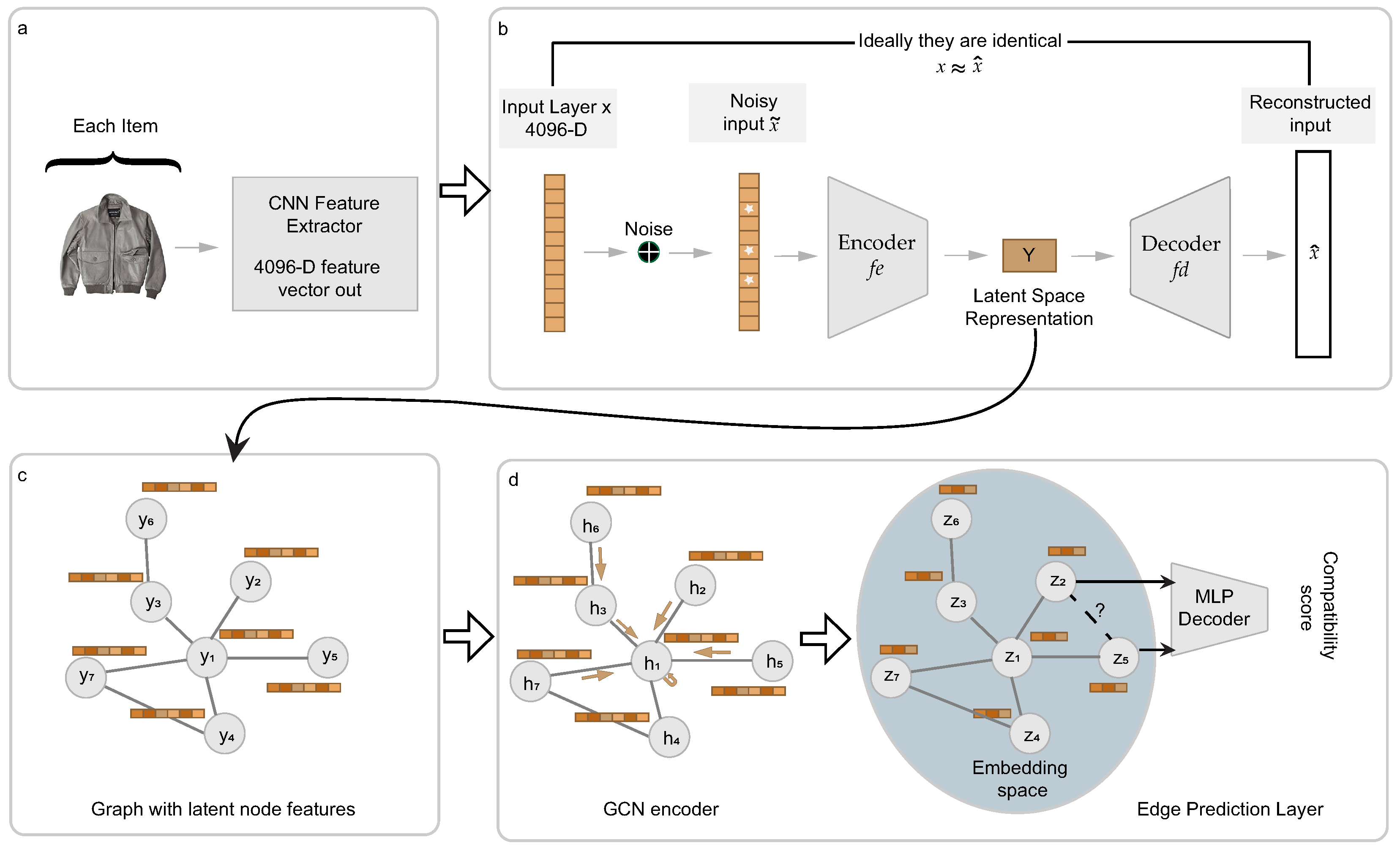
Figure 1. The diagram illustrates the model for predicting the compatibility scores of fashion items. (a) Feature extraction using CNN-F architecture produces a 4096-dimensional vector x from each fashion image, capturing detailed image features. (b) A deep-stacked autoencoder transforms these features into a latent space y, optimizing for subsequent processing. (c) We construct a relational graph by effectively merging item interactions (e.g., ’also viewed’, ’also bought’, ’bought together’) with node latent features, thereby enhancing data relational insights. (d) A tailored GCN encoder refines the graph, and then an edge prediction layer computes item compatibility scores.
Make 06 00104 g001
Figure 2. The diagram illustrates the GCN workflow, which begins with the initial input graph, which contains 256 node features. Subsequent graph convolution layers reduce the dimensionality to 64 features, utilizing ReLU activations for nonlinear transformations. The process concludes in the embedding space, where an MLP decoder utilizes node embeddings to calculate compatibility scores between nodes.
Make 06 00104 g002
Figure 3. ROC Curves for the Women’s and Men’s category interactions across different k values, showing the AUC metrics.
Make 06 00104 g003
Figure 4. Training and Validation Loss Trends for the VAGCN, demonstrating effective error minimization and consistent performance throughout the training process.
Make 06 00104 g004
Figure 5. Test Accuracy versus Neighborhood Size (k-values) for Men’s and Women’s Categories, indicating accuracy stabilization beyond k = 20 for various interaction types.
Make 06 00104 g005
Figure 6. Training loss and accuracy comparison between the GCN configurations (256, 128, 64) and Uniform GCN (256 × 3), showcasing the superior stability and efficiency of the decreasing layer size model.
Make 06 00104 g006
Figure 7. Performance comparison of different learning rates, indicating how a 0.01 learning rate achieves an optimal balance between rapid convergence and robust generalization.
Make 06 00104 g007
Figure 8. Visualization of link predictions in a women’s fashion test dataset, illustrating compatibility scores between item pairs. The scores are normalized between 0 and 1, where values closer to 1 indicate high compatibility and values closer to 0 denote low compatibility.
Make 06 00104 g008
Table 1. Notations and Descriptions.
NotationDescription
xOriginal input data
x ˜ Noisy version of input data
YLatent representation of data
x ^ Reconstructed version of original input data
W , W Weight matrices represent the encoder and decoder, respectively.
b , b Vectors represent the bias vectors for the encoder and decoder, respectively.
f e , f d The activation functions for the encoder and decoder, respectively
G = ( V , E ) Graph contains nodes V and edges E
XNode feature matrix
dDimensionality of feature vector
H ( l ) Node representation after l graph convolutional layers
D ˜ Normalized Laplacian matrix
p i j Predicted probability of an edge between nodes i and j
h i ( L ) , h j ( L ) Representations of nodes i and j at the L-th layer, respectively
PProbability matrix indicating the likelihood of edges between nodes.
AAdjacency matrix of the graph
Table 2. Statistics of each dataset categorized by relation.
CategoryRelation# Nodes# EdgesAvg. Degree
Menalso_viewed105,462787,04813.80
bought_together30,41545,1602.85
also_bought49,660441,98716.52
Womenalso_viewed263,3122,692,36618.97
bought_together93,726155,3443.19
also_bought121,9631,771,17326.97
Boysalso_viewed669524,3807.04
bought_together230625722.17
also_bought589722,4607.42
Girlsalso_viewed19,854103,9389.85
bought_together567169622.38
also_bought11,96263,82210.15
Babyalso_viewed11,25878,14813.31
bought_together625096813.03
also_bought11,148113,02119.66
Table 3. Accuracy of VAGCN and baseline models across top-level categories for also_viewed, also_bought, and bought_together interactions, detailing performance at neighborhood settings k = 10 . The bold indicates the best accuracy in each category.
CategoryMethodAlso_ViewedAlso_BoughtBought_Together
MenCT88.2%78.4%83.6%
WNN86.9%78.4%82.3%
McAuley et al. k = 10 91.6%89.8%92.1%
VAGCN k = 10 (Ours)97.1%95.9%94.4%
WomenCT86.8%79.1%84.3%
WNN78.8%76.1%80.0%
McAuley et al. k = 10 88.9%87.8%91.5%
VAGCN k = 10 (Ours)96.7%93.9%94.9%
BoysCT81.9%77.3%83.1%
WNN85.0%87.2%87.9%
McAuley et al. k = 10 94.4%94.1%93.8%
VAGCN k = 10 (Ours)96.1%96.0%94.5%
GirlsCT83.0%76.2%78.7%
WNN83.3%86.0%84.8%
McAuley et al. k = 10 94.5%93.6%93.0%
VAGCN k = 10 (Ours)96.8%95.8%93.9%
BabyCT77.1%70.5%80.1%
WNN83.0%87.7%81.7%
McAuley et al. k = 10 92.2%92.7%91.5%
VAGCN k = 10 (Ours)96.7%95.1%92.9%
Disclaimer/Publisher’s Note: The statements, opinions and data contained in all publications are solely those of the individual author(s) and contributor(s) and not of MDPI and/or the editor(s). MDPI and/or the editor(s) disclaim responsibility for any injury to people or property resulting from any ideas, methods, instructions or products referred to in the content.