Improving Time Series Regression Model Accuracy via Systematic Training Dataset Augmentation and Sampling

Abstract

This study addresses a significant gap in the field of time series regression modeling by highlighting the central role of data augmentation in improving model accuracy. The primary objective is to present a detailed methodology for systematic sampling of training datasets through data augmentation to improve the accuracy of time series regression models. Therefore, different augmentation techniques are compared to evaluate their impact on model accuracy across different datasets and model architectures. In addition, this research highlights the need for a standardized approach to creating training datasets using multiple augmentation methods. The lack of a clear framework hinders the easy integration of data augmentation into time series regression pipelines. Our systematic methodology promotes model accuracy while providing a robust foundation for practitioners to seamlessly integrate data augmentation into their modeling practices. The effectiveness of our approach is demonstrated using process data from two milling machines. Experiments show that the optimized training dataset improves the generalization ability of machine learning models in 86.67% of the evaluated scenarios. However, the prediction accuracy of models trained on a sufficient dataset remains largely unaffected. Based on these results, sophisticated sampling strategies such as Quadratic Weighting of multiple augmentation approaches may be beneficial.

1. Introduction

The use of machine learning (ML) for industrial applications is increasingly gaining traction [1,2], leading to new challenges arising from real-world applications. Developing predictive models requires a sufficiently large and representative dataset [3], a condition that is challenging to achieve in industrial settings [4]. Particularly in manufacturing, this challenge is exacerbated by rapidly changing markets and the demand for customized production with batch sizes as small as one part [5]. The resulting rapid change in production results in a lack of training data. One approach to overcoming this challenge is to apply data augmentation. By systematically augmenting data, higher accuracy and improved robustness can be achieved [6]. Numerous approaches have been developed, particularly in image generation, which are the starting point for integrating technical problems. For example, integrating data augmentation can increase the maximum validation accuracy for pitting classification on ball screw drives [7]. Recently, research has intensified on augmentation methods for time series data [8], which has the potential to increasingly enable ML approaches in low-data regimes. An example is the identification of failure modes in machine components such as ball bearings, where typically only a few specific data points are available to describe a failure pattern. Here, Ref. [9] demonstrated that using augmented signals can lead to better classification results. In addition, Ref. [10] showed that using augmented data enables efficient training of ML models for determining faulty machine states, especially with a small number of faulty samples. As represented in [11] for spatial and frequency domain-based argumentation, Generative Adversarial Networks (GAN) are now incorporated into classifying fault conditions in the industrial context.

Building on statistics, a thoughtful compilation of training datasets has long been in focus. Describing complex problems or conducting experiments can be laborious and costly when searching for representative data points through real-world setups. Adding artificially generated data points can help to reduce the amount of necessary experiments. A major challenge is the time-efficient assembly of suitable training datasets, which are highly relevant. For example, Ref. [12] developed an efficient Markov Chain Monte Carlo algorithm for sampling posterior distributions by combining marginal and conditional augmentation. The following sections review the current state of the art in image and time series augmentation approaches.

1.1. Augmentation for Image Data

Data-driven approaches to image processing have gained prominence due to the increasing use of cameras, e.g., for object recognition. Consequently, there has been a significant focus on image augmentation for classification tasks. By augmenting data in the feature space, domain-independent approaches can be developed [13]. However, data space augmentation has a greater impact on classification performance improvement and overfitting reduction than feature space augmentation [14]. Examining the effects of linear transformations, Ref. [15] showed that label-invariant augmentation can improve accuracy by adding information and that label-mixing approaches can improve accuracy through regularization effects. Thus, combinations of images can be used for augmentation in addition to modifying individual images by rotation, noise, or distortion. Furthermore, a systematic augmentation strategy dominates over random augmentation in the context of image classification [6]. For example, classification results can be improved by generating augmented data points based on the distribution of the training dataset [16]. In [17], an approach was presented with the aim of generating data points as close as possible to those of the original dataset while maximizing information. Due to the variety of approaches to image augmentation, the compilation of training datasets is becoming increasingly important. In [18], the the best results were achieved using a combination of augmentation methods. Augmentation and weighting can be used to dynamically adjust datasets, which is especially beneficial in low-data regimes and scenarios involving class imbalance [19]. Likewise, Ref. [20] showed that the training dataset’s compilation can be considered part of the training process and that appropriate data augmentation policies can be learned.

1.2. Augmentation for Time Series Data

In recent years, increasing attention has been paid to augmenting time series data, especially for classification tasks. Similar to image data, simple approaches such as adding noise, distortion (warping), or flipping can be applied [8]. Using the example of biosignals classification, Ref. [21] demonstrated that adding augmented data is particularly efficient, especially with small datasets, achieving nearly the same level of accuracy as when using a larger dataset. Generating time series with respect to the characteristics of the original dataset produces better results than generating time series with multiple characteristics [22]. Starting from this, more advanced methods have recently been developed. For example, Ref. [23] described an augmentation approach based on Dynamic Time Warping (DTW). Using a DTW-based augmentation approach, Ref. [24] demonstrated that Convolutional Neural Network structures can learn time-invariant features. In [25], the authors conducted a comprehensive review of data augmentation methods for time series and their application in the context of classification with neural networks. In another study [26], a significant improvement in accuracy was achieved by using traditional augmentation approaches. In contrast, the additional use of generative approaches such as variational autoencoders could reduce the variance of the 5-fold cross-validation. There is growing use of GANs for time series; however, it remains a niche area with major limitations, namely, the length of the generated time series and its application-specific nature, with poor generalizability across domains [27]. Similar to [28], the authors of [29] showed that a dataset created by a GAN adapted for unevenly sampled time series could achieve similar classification accuracy as the original dataset. In [30], several state-of-the-art neural network-based approaches were explored, leading to the suggestion that performance can be enhanced using a balanced ensemble. Using network traffic data as an example, Ref. [31] showed that two publicly available GANs—TimeGAN and DoppleGANger—were able to outperform a probabilistic autoregressive model. Many applications are currently being explored, e.g., [32] offers GAN-based augmentation using a biosignal classification problem.

1.3. Summary and Research Deficit

As with to image data, the development of augmentation approaches for time series started with simple methods and has progressed to more advanced ones such as GANs. Similar to image augmentation, the focus in time series augmentation has been on general augmentation (e.g., [8,24,32]) or the improvement of ML-based classifiers (e.g., [21,25,29]), either through increasing overall performance or through the expansion of underrepresented classes. As a result, a wide range of applicable approaches is available today. Despite its high industrial relevance, the impact of data augmentation in the context of time series prediction, which can be understood as a regression problem, remains a relatively young field and there is a lack of knowledge regarding the impact of augmented data on the prediction of regression models, especially in industrial contexts. It can be assumed that improvements in accuracy can be achieved by using multiple augmentation sets via an appropriate sampling strategy. This assumption is further emboldened by the results in [8], emphasizing the development of efficient selection and combination strategies for time series augmentation as a future research direction. A deeper analysis of ensemble techniques is further motivated by [30].

To address these shortcomings, a general framework for constructing training datasets using augmented data and subsequent retraining specifically tailored for machine learning models is presented here. This framework is applied to the prediction of Computer Numerical Controlled (CNC) axis current signals across different datasets, providing the basis for investigating the impact of augmented data and the composition of training datasets on the performance of machine learning models.

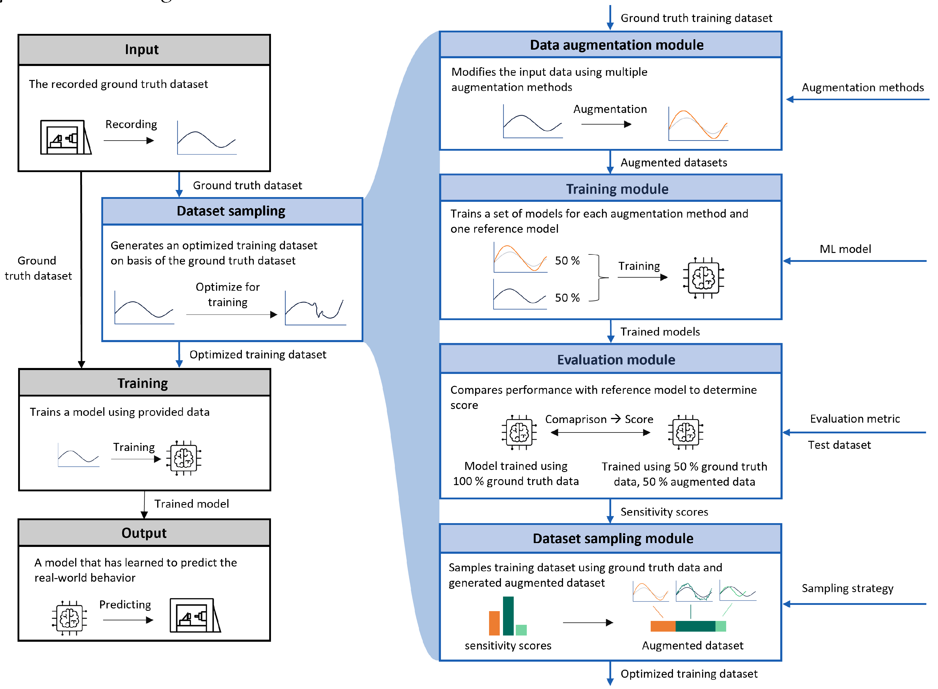
2. Framework for Training Dataset Sampling

Augmentation methods have specific effects on the prediction quality of regression models. For example, robustness can be increased by adding noise, while accuracy can be improved by generating underrepresented segments. In addition, these effects interact with each other to further influence the trained model. The proposed framework aims to extend traditional training approaches by systematically identifying the influences of a set of given augmentation methods. Based on the improvements, an optimized dataset is sampled and the model is then retrained. The overall approach is illustrated in Figure 1. Each module is described in more detail below.

Input: Similar to traditional model training, the input to the dataset sampling framework is a given dataset. This represents the ground truth dataset, which is divided into a ground truth training dataset and a test dataset. These are used to train and evaluate the ML models.

Data Augmentation Module: The data augmentation module contains N augmentation methods n for the generation of synthetic data. Every method that generates datasets based on given ground truth data can be used in this module. Each method creates an augmented dataset of the same size as the ground truth training dataset. For each method, the module outputs one augmented dataset.

Training Module: This module handles model training. A training dataset is created for each augmentation method, consisting of the ground truth training dataset and the augmented dataset. Similar to the literature, the real-to-synthetic ratio is set to be equal. Using these augmentation method-specific training datasets, the ML model to be optimized is trained as an ensemble to account for statistical uncertainties in model training and overfitting. These ensembles of trained models are then passed to the evaluation module.

Evaluation Module: For this module, a metric must be defined against which the models will be evaluated, for example, classification accuracy or mean squared error (MSE) in the case of regression problems. All trained models are evaluated on the separated test dataset and compared to the performance of the ground truth model trained via the ground truth training dataset. The sensitivity score S is calculated as the difference in terms of a given evaluation metric (e.g., MSE) between the performance of the model trained on the augmented dataset and the model trained on the ground truth training dataset, quantifying how the augmentation affects model performance. Thus, high sensitivity scores indicate strong model performance improvement, while a score below zero indicates a decrease in model performance.

Dataset Sampling Module: The core of this novel approach is the dataset sampling module. Its goal is to generate an optimized training dataset based on combining the ground truth training dataset with synthetic data from multiple augmentation methods. Therefore, the ratio for the synthetic part of the training dataset has to be defined based on a chosen real-to-synthetic ratio. For each augmentation method, the weighted sum of the sensitivity scores S calculated via the evaluation module defines the amount of augmented data used in the optimized training dataset. The weighting has to be defined by the sampling strategy. Augmentation methods with negative scores did not improve model performance, and as such were excluded.

Training: The training process of the desired model is not changed. The same model and algorithm can be used as in the classical approach. The only difference is in the input data; instead of using only the ground truth data, the optimized training dataset consisting of ground truth data and augmented data is used to train the model.

Output: The model is output from the framework after it has been trained via the optimized training dataset.

3. Study and Methology

The presented framework was investigated in an industrial context. Due to the complex coupling between machine and process variables, milling machines are particularly suitable for time series prediction. If it is possible to predict the current signals of individual axes, they can be used for process- and part-independent predictions. This allows processes to be monitored from part one, meaning that it is no longer necessary to determine reference signals beforehand by recording them. For this purpose, the proposed framework is tested on the approach introduced in [33]. In the presented hybrid model, an ML model maps previously simulated kinematic quantities such as axis-specific velocities, accelerations, and process forces onto the current signals of the X, Y, and Z-axes and the main spindle (SP) of a milling machine with a target frequency of 50 Hz. These current signals are sampled from a continuous process; thus, according to [27], this is defined as a continuous time series problem on $t\in [t=0\dots t=t_{\max }]$.

3.1. Datasets and Experiments

Two datasets were used for the presented study, both consisting of recordings of machine data from a milling machine taken during the production of two distinct parts. The first dataset [34] was recorded on a DMC 60 H milling machine from DECKEL MAHO (produced by DMG MORI Aktiengesellschaft, Bielefeld, Germany), while the second [35] was recorded on a CMX 600 V milling machine from DMG MORI (produced by DMG MORI Aktiengesellschaft, Bielefeld, Germany). The recorded data included current signals from the axis and spindle motors as well as their speed and acceleration. By selecting data from two different machines, conclusions can be drawn about machine-specific influences, ensuring the generalizability of the approach and its results.

The derived experiments were designed to investigate two application cases. Experiment 1 was designed to evaluate influences on prediction quality during the production of a known part. For this purpose, recordings of the same part’s process were used for the training and test set. In Experiment 2, influences on the prediction quality of an unseen part were investigated. For this purpose, recordings of the manufacturing process of two different parts were used. The models were trained on the recordings of the first part, while the recordings of the second part were used for model testing, allowing influences on the generalization ability of the models to be investigated. Both experiments were performed for both the CMX 600 V (A) and DMC 60 H (B) datasets. In each case, models were trained for each axis and for the main spindle. Information about the implementation can be found in Appendix A.

3.2. Models

The models were used to predict the axis currents of a milling machine. Values were predicted for each timestamp in a time series based on speed v, acceleration a, process forces f, and the material removal rate MRR of the X, Y, and Z axes and the SP. To better model the machine’s physical properties and the axes’ controller, data points up to 0.04 s before and after the timestep were included in the input vector. Thus, the results for the X-axis-specific input vector for timestamp t in _{X, t} is calculated as follows:

$${in}_{\mathrm{X},\mathrm{t}}=\left(\begin{array}{c}{v}_{\mathrm{X},\mathrm{t}}\\ a_{\mathrm{X},\mathrm{t}}\\ f_{\mathrm{X},\mathrm{t}}\end{array}\right),wi\mathrm{t}ht\in [-40\mathrm{ms},-20\mathrm{ms},0\mathrm{ms},20\mathrm{ms},40\mathrm{ms}].$$

The input vector is calculated as follows:

$${in}_{\mathrm{t}}=\left(\begin{array}{c}{in}_{\mathrm{X},\mathrm{t}}\\ {in}_{\mathrm{Y},\mathrm{t}}\\ {in}_{\mathrm{Z},\mathrm{t}}\\ {in}_{\mathrm{S}\mathrm{P},\mathrm{t}}\\ {MMR}_{\mathrm{t}}\end{array}\right),wi\mathrm{t}ht\in [-40\mathrm{ms},-20\mathrm{ms},0\mathrm{ms},20\mathrm{ms},40\mathrm{ms}].$$

For each axis and the main spindle, the output of the specific model M is a single value representing the predicted current at a given timestamp

$${out}_{\mathrm{X},\mathrm{t}}=M_{\mathrm{X}}\left({in}_{\mathrm{t}}\right),{out}_{\mathrm{Y},\mathrm{t}}=M_{\mathrm{Y}}\left({in}_{\mathrm{t}}\right),{out}_{\mathrm{Z},\mathrm{t}}=M_{\mathrm{Z}}\left({in}_{\mathrm{t}}\right)and{out}_{\mathrm{S}\mathrm{P},\mathrm{t}}=M_{\mathrm{S}\mathrm{P}}\left({in}_{\mathrm{t}}\right).$$

To ensure comparability, tests were performed on four different model architectures. In general, the study of dataset sampling strategies should be carried out using common model structures, as these provide understandable insights into the resulting effects. Thus, two neural networks NN and two random forests RF were chosen. A higher model complexity (more layers, higher maximum depth) can be suitable for mapping more complex relationships. Due to the higher number of parameters to be determined, a larger training dataset can have a greater impact. To investigate the influence of different complexities, both types were implemented using both a simpler S and a more complex C model structure. The most relevant hyperparameters are summarized in

Table 1. Key hyperparameters of the chosen neural network NN and random forest RF models.

Name	Hidden Layers	Hidden Dimensions	Epochs	Learning Rate	Optimizer
$N{N}_{\mathrm{S}}$	2	64	1000	0.001	Adam
$N{N}_C$	7	128	1000	0.001	Adam
Name	Estimators	Maximum Depth	Split Minimum	Leaf Minimum	Criteriom
$R{F}_{\mathrm{S}}$	10	3	2	1	squared error
$R{F}_C$	10	20	2	1	squared error

, highlighting the differences between the simple and complex model structures. This approach makes it possible to study the effect of data augmentation and dataset sampling on different model architectures and complexities.

3.3. Augmentation Methods

Several augmentation methods can be used to generate synthetic data. Especially in recent years, deep generative models (DGMs) such as GANs have been increasingly used to generate data [27]. The quality of the generated data depends strongly on the implementation of the DGMs [36]. As optimal implementation is very time-consuming and requires a high level of expertise, this work focuses on several simple and well proven methods.

Magnitude Warping: The goal of magnitude warping is to change the position of the data in the target domain. The implementation was based on [37]. Therefore, a spline polynomial of the same length as the time series is generated. The spline polynomial is then used for an element-wise multiplication for each value of the time series.

Noise: Adding noise to a given signal is a common augmentation method.

Random Deletion: For this augmentation method, random data points in the time series are deleted. This corresponds to randomized temporal compression of the signal at these points.

Time Warping: Similar to magnitude warping, time warping uses a spline polynomial to magnify a given signal. In contrast to random deletion, there is systematic compression and stretching in the time domain. The implementation for this method followed [37].

Window Warping: Window warping was performed according to [38]. In this process, a randomly selected portion of the time series is either compressed to half its length or stretched to twice its length.

3.4. Dataset Sampling Strategies

This study used datasets with a real-to-synthetic ratio of 1, which has been proven in [39] to be an appropriate rate. Three dataset sampling strategies were investigated to determine the percentage $P_n$ of the training dataset to be filled with data from each augmentation method:

Highest: Only synthetic data from the method with the highest sensitivity score S are used for dataset sampling. This approach represents a winner-takes-it-all strategy, and is often used in the existing literature. After testing N augmentation methods, the best one is chosen, and $P_n$ results in

$$P_n=\left\{\begin{array}{cc}100\%\hfill & \mathrm{if}{S}_n=max(S_1,S_2,\dots ,S_N)\hfill \\ 0\%\hfill & \mathrm{otherwise}\hfill \end{array}\right..$$

(1)

Linear Weighting: The training dataset is sampled using the weighted sum of the augmented datasets based on the sensitivity score S. Thus, $P_n$ results in

$$P_n=\frac{S_n}{{\sum }_{i=1}^N{S}_i}\times 100\%.$$

(2)

Quadratic Weighting: Similar to linear weighting, the weighted sum is calculated. Here, each weight $P_n$

$$P_n=\frac{S_n^2}{{\sum }_{i=1}^N{S}_i^2}\times 100\%$$

(3)

is squared, resulting in a stronger weighting of methods with higher sensitivity scores S.

3.5. Evaluation Metrics

The purpose of this study was to determine the influence of augmented and sampled training data on the accuracy of a regression model using the example of predicting the current signals of the axes of a machine tool. In order to meet this manufacturing context, metrics related to the possible application of the model were used. As the resulting values of the regression model are estimated motor currents, they can be used to predict the energy consumption of a production process. Thus, the accuracy of the model increases as the difference between the integral of the predicted signal and the recorded signal decreases. The percentage deviation

$$DEV=\frac{X_{est}-X_{meas}}{X_{meas}}\times 100$$

(4)

between the integrals provides the estimated deviation, where:

• $DEV$ is the total deviation in %,
• $X_{est}$ is the integral of the absolute of the predicted current, i.e., $X_{est}={\int }_0^{t_{\max }}\left|I_{est}\left(t\right)\right|dt$,
• $X_{meas}$ is the integral of the absolute of the measured current, i.e., $X_{meas}={\int }_0^{t_{\max }}\left|I_{meas}\left(t\right)\right|dt$.

The commonly used Mean Squared Error (MSE) better highlights local and large deviations between predicted and actual time series. This is especially important if the model is to be used for anomaly detection. Therefore,

$$MSE=\frac{1}{T}\sum _{i=1}^T{(x_i-{\widehat{x}}_i)}^2$$

(5)

was used as a second evaluation metric, where T is the total number of points in the time series, x is the actual value, and $\widehat{x}$ is the predicted value.

4. Results

The effects of an isolated application of the augmentation methods (Section 3.3) on the prediction quality of time series regression models were examined via the evaluation metrics MSE and DEV (Section 3.5). Building on this, we investigate the influence of a combination of the approaches in Section 3.1.

4.1. Impact of Augmentation Methods

The influence of the chosen augmentation methods was tested by training and evaluating the ML models defined in Section 3.2 using a real-to-synthetic ratio of 1. Based on Experiments 1 and 2 (A/B), explained in Section 3.1, models were trained for the X-, Y-, and Z-axes and for the main spindle of the two milling machines. The averaged results and listed in

Table 2. Evaluation of ML models trained with a real-to-synthetic ratio of 1. The values shown are the average MSE and DEV of the NC axis (X, Y, Z) and SP. For X, Y, Z, and SP, the mean value of ten replications is used. The entry with the best result for the respective metric is highlighted. The standard deviation of the averaging is shown in brackets.

Axis	Model	Original Dataset	Magnitude Warping	Noise	Random Delete	Time Warping	Window Warping
Experiment 1A (DEV)	$R{F}_{\mathrm{S}}$	6.58 (0.08)	3.24 (3.52)	5.77 (0.14)	6.52 (0.03)	6.04 (1.02)	5.94 (0.57)
	$R{F}_C$	1.12 (0.80)	1.20 (0.16)	0.93 (0.02)	0.86 (0.11)	0.94 (0.42)	1.07 (0.57)
	$N{N}_{\mathrm{S}}$	1.60 (0.52)	3.71 (0.64)	1.33 (0.47)	3.51 (0.48)	2.31 (0.44)	1.88 (0.50)
	$N{N}_C$	1.80 (1.81)	2.17 (3.00)	1.49 (1.34)	2.43 (1.16)	2.22 (2.13)	1.86 (1.56)
Experiment 1A (MSE)	$R{F}_{\mathrm{S}}$	0.22 (0.00)	0.65 (0.14)	0.45 (0.00)	0.38 (0.00)	0.38 (0.01)	0.45 (0.00)
	$R{F}_C$	0.05 (0.00)	0.17 (0.00)	0.15 (0.00)	0.16 (0.01)	0.16 (0.01)	0.18 (0.03)
	$N{N}_{\mathrm{S}}$	0.11 (0.00)	0.32 (0.04)	0.27 (0.00)	0.28 (0.00)	0.28 (0.02)	0.27 (0.00)
	$N{N}_C$	0.06 (0.01)	0.30 (0.03)	0.27 (0.02)	0.27 (0.01)	0.26 (0.01)	0.27 (0.02)
Experiment 1B (DEV)	$R{F}_{\mathrm{S}}$	7.83 (0.04)	5.30 (4.61)	8.45 (2.73)	3.00 (0.42)	4.69 (1.18)	7.78 (0.52)
	$R{F}_C$	0.74 (0.08)	0.59 (0.17)	0.87 (0.63)	0.72 (0.56)	0.73 (0.26)	0.76 (0.11)
	$N{N}_{\mathrm{S}}$	0.76 (0.53)	1.45 (0.82)	0.90 (0.46)	1.12 (0.63)	1.15 (0.64)	1.31 (1.34)
	$N{N}_C$	1.41 (1.47)	1.70 (3.11)	2.60 (2.18)	2.96 (2.02)	1.96 (2.32)	1.59 (2.01)
Experiment 1B (MSE)	$R{F}_{\mathrm{S}}$	0.36 (0.00)	0.64 (0.14)	0.46 (0.01)	0.68 (0.02)	0.69 (0.01)	0.35 (0.02)
	$R{F}_C$	0.01 (0.00)	0.03 (0.00)	0.02 (0.00)	0.01 (0.00)	0.03 (0.01)	0.01 (0.00)
	$N{N}_C$	0.47 (0.02)	0.50 (0.02)	0.53 (0.01)	0.52 (0.01)	0.51 (0.01)	0.49 (0.02)
	$N{N}_{\mathrm{S}}$	0.25 (0.59)	0.24 (0.04)	0.36 (0.07)	0.45 (0.04)	0.31 (0.06)	0.24 (0.13)
Experiment 2A (DEV)	$R{F}_{\mathrm{S}}$	9.59 (2.96)	15.14 (6.82)	8.68 (3.95)	27.75 (4.41)	23.72 (3.19)	8.99 (3.31)
	$R{F}_C$	5.51 (4.88)	7.58 (6.89)	4.07 (3.24)	27.33 (6.07)	26.67 (6.21)	13.40 (4.28)
	$N{N}_{\mathrm{S}}$	15.33 (6.06)	32.93 (6.71)	10.91 (6.39)	17.09 (4.45)	17.88 (4.36)	13.96 (4.10)
	$N{N}_C$	21.23 (7.31)	28.12 (7.02)	12.67 (6.68)	13.44 (5.59)	10.73 (5.10)	14.64 (6.46)
Experiment 2A (MSE)	$R{F}_{\mathrm{S}}$	0.41 (0.03)	1.74 (0.24)	2.06 (0.02)	2.03 (0.01)	2.05 (0.02)	2.07 (0.01)
	$R{F}_C$	0.39 (0.04)	1.75 (0.33)	2.08 (0.02)	2.19 (0.02)	2.20 (0.01)	2.23 (0.04)
	$N{N}_{\mathrm{S}}$	0.53 (0.12)	1.48 (0.08)	1.55 (0.06)	1.38 (0.04)	1.35 (0.04)	1.45 (0.09)
	$N{N}_C$	1.43 (0.43)	1.46 (0.10)	1.65 (0.06)	1.57 (0.07)	1.69 (0.09)	1.59 (0.06)
Experiment 2B (DEV)	$R{F}_{\mathrm{S}}$	1.00 (0.40)	5.98 (8.33)	1.07 (0.64)	6.16 (0.98)	2.08 (1.70)	2.80 (1.04)
	$R{F}_C$	4.20 (4.67)	5.08 (4.33)	5.10 (4.15)	4.74 (4.31)	6.52 (5.92)	5.11 (4.10)
	$N{N}_{\mathrm{S}}$	9.44 (4.44)	8.40 (4.72)	7.64 (2.35)	10.19 (5.93)	8.70 (3.74)	9.10 (3.62)
	$N{N}_C$	11.50 (6.22)	8.95 (7.22)	6.54 (4.46)	8.09 (7.86)	6.42 (7.44)	9.59 (7.17)
Experiment 2B (MSE)	$R{F}_{\mathrm{S}}$	0.99 (0.01)	1.53 (0.19)	1.09 (0.07)	1.57 (0.02)	1.57 (0.02)	1.18 (0.10)
	$R{F}_C$	0.69 (0.07)	0.87 (0.15)	0.88 (0.06)	0.85 (0.07)	1.24 (0.28)	0.85 (0.13)
	$N{N}_{\mathrm{S}}$	3.24 (1.27)	2.66 (0.75)	2.48 (0.13)	2.10 (0.34)	3.14 (0.70)	3.23 (1.61)
	$N{N}_C$	32.71 (21.09)	1.81 (0.31)	3.92 (0.47)	1.65 (0.34)	4.10 (2.34)	11.96 (12.18)

, with the standard deviation shown in brackets after the result.

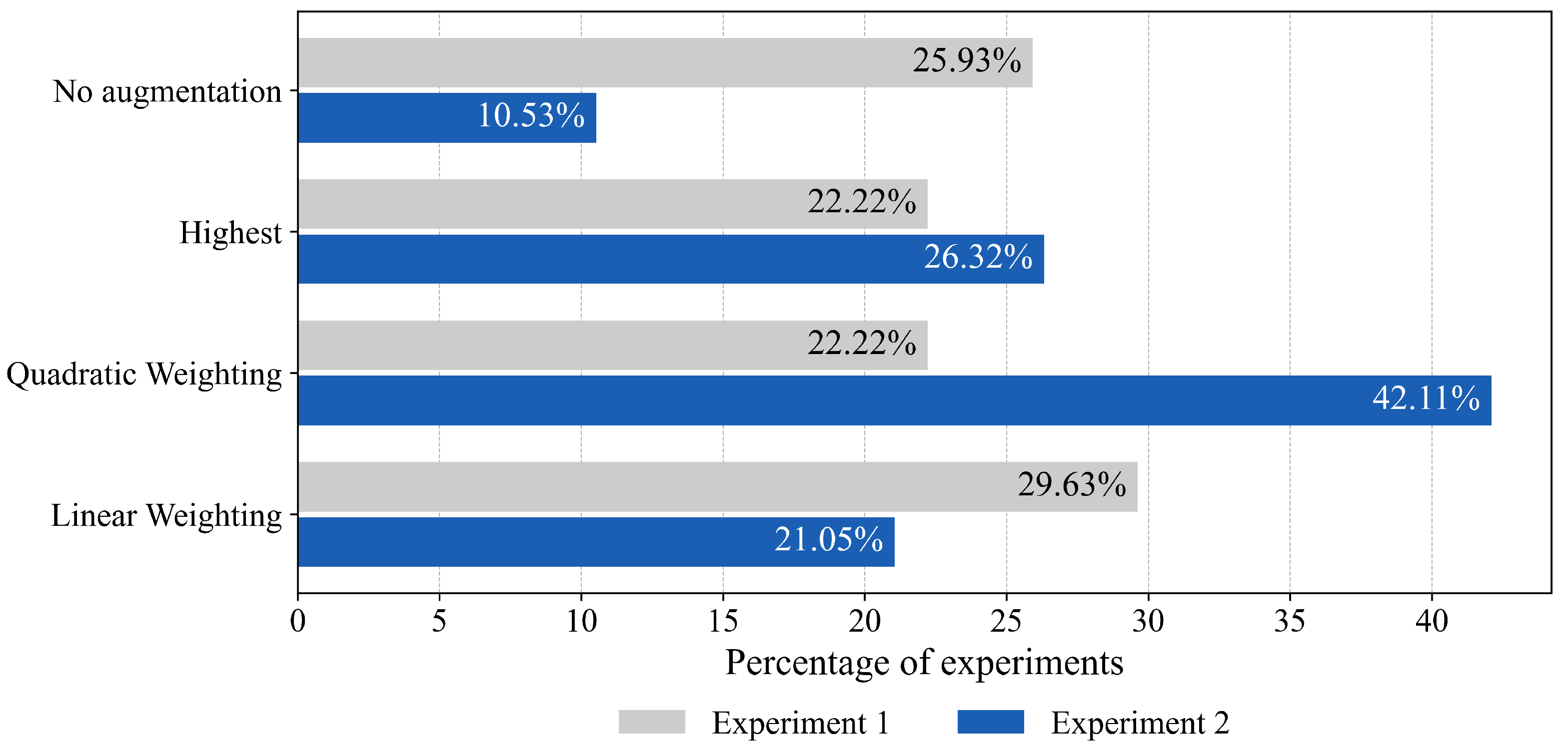
4.2. Impact of Dataset Sampling Strategies

Optimized training datasets were generated for each experiment using the proposed dataset sampling strategy and a real-to-synthetic ratio of 1. The synthetic part of the optimized training dataset was then sampled according to the sampling strategies described in Section 3.4. Therefore, the training dataset in this experimental setup consists of the ground truth training dataset enriched with the same amount of the $P_n$-weighted augmented datasets. The mean and standard deviation of DEV and MES were calculated for ten models trained in each experiment. The evaluation results are listed in

Table 3. Evaluation of ML models trained using sampled datasets. The values shown are the average MSE and DEV of the NC axis (X, Y, Z) and SP. For X, Y, Z, and SP, the mean value of ten replications is used. The entry with the best result for the respective metric is highlighted. The standard deviation is shown in brackets.

Axis	Model	Original Dataset	$\mathit{Highest}$	$\mathit{Quadratic}\mathit{Weighting}$	$\mathit{Linear}\mathit{Weighting}$
Experiment 1A (DEV)	$R{F}_{\mathrm{S}}$	6.58 (0.08)	5.50 (0.21)	5.68 (0.23)	5.67 (0.15)
	$R{F}_C$	1.12 (0.80)	0.94 (0.06)	1.00 (0.05)	0.98 (0.06)
	$N{N}_{\mathrm{S}}$	1.60 (0.52)	1.32 (0.45)	1.43 (0.55)	1.29 (0.53)
	$N{N}_C$	1.80 (1.81)	1.86 (1.30)	2.67 (3.08)	0.72 (1.68)
Experiment 1A (MSE)	$R{F}_{\mathrm{S}}$	0.22 (0.00)	0.22 (0.00)	0.23 (0.00)	0.22 (0.00)
	$R{F}_C$	0.05 (0.00)	0.05 (0.00)	0.05 (0.00)	0.05 (0.00)
	$N{N}_{\mathrm{S}}$	0.11 (0.00)	0.11 (0.00)	0.11 (0.00)	0.11 (0.00)
	$N{N}_C$	0.06 (0.01)	0.08 (0.01)	0.08 (0.02)	0.08 (0.02)
Experiment 1B (DEV)	$R{F}_{\mathrm{S}}$	7.83 (0.04)	7.79 (0.24)	7.67 (0.12)	7.72 (0.13)
	$R{F}_C$	0.74 (0.08)	0.76 (0.11)	0.71 (0.12)	0.74 (0.14)
	$N{N}_{\mathrm{S}}$	0.76 (0.53)	0.80 (0.39)	1.02 (0.77)	0.85 (0.58)
	$N{N}_C$	1.41 (1.47)	1.14 (1.05)	1.29 (1.69)	1.71 (2.39)
Experiment 1B (MSE)	$R{F}_{\mathrm{S}}$	0.36 (0.00)	0.36 (0.00)	0.35 (0.01)	0.35 (0.01)
	$R{F}_C$	0.01 (0.00)	0.01 (0.00)	0.02 (0.00)	0.01 (0.00)
	$N{N}_{\mathrm{S}}$	0.47 (0.02)	0.53 (0.01)	0.52 (0.01)	0.53 (0.01)
	$N{N}_C$	0.25 (0.59)	0.20 (0.02)	0.25 (0.07)	0.19 (0.03)
Experiment 2A (DEV)	$R{F}_{\mathrm{S}}$	9.59 (2.96)	8.85 (2.83)	9.40 (1.76)	9.39 (4.46)
	$R{F}_C$	5.51 (4.88)	4.84 (2.22)	5.00 (2.48)	3.88 (3.68)
	$N{N}_{\mathrm{S}}$	15.33 (6.06)	10.80 (5.66)	7.98 (6.39)	10.83 (5.10)
	$N{N}_C$	21.23 (7.31)	21.66 (4.90)	12.60 (6.86)	11.42 (5.46)
Experiment 2A (MSE)	$R{F}_{\mathrm{S}}$	0.41 (0.03)	0.39 (0.02)	0.40 (0.02)	0.40 (0.02)
	$R{F}_C$	0.39 (0.04)	0.40 (0.08)	0.40 (0.05)	0.39 (0.06)
	$N{N}_{\mathrm{S}}$	0.53 (0.12)	0.42 (0.08)	0.37 (0.04)	0.46 (0.11)
	$N{N}_C$	1.43 (0.43)	1.99 (0.64)	1.12 (0.25)	1.55 (0.35)
Experiment 2B (DEV)	$R{F}_{\mathrm{S}}$	1.00 (0.40)	0.97 (0.42)	1.39 (0.86)	1.13 (0.38)
	$R{F}_C$	4.20 (4.67)	4.15 (4.68)	4.05 (4.01)	3.47 (2.45)
	$N{N}_{\mathrm{S}}$	9.44 (4.44)	9.17 (3.45)	7.38 (1.55)	8.64 (2.93)
	$N{N}_C$	11.50 (6.22)	8.62 (7.83)	7.35 (4.67)	7.48 (5.57)
Experiment 2B (MSE)	$R{F}_{\mathrm{S}}$	0.99 (0.01)	0.97 (0.04)	0.98 (0.04)	0.99 (0.05)
	$R{F}_C$	0.69 (0.07)	0.71 (0.05)	0.69 (0.09)	0.71 (0.03)
	$N{N}_{\mathrm{S}}$	3.24 (1.27)	2.30 (0.21)	2.30 (0.15)	2.47 (0.22)
	$N{N}_C$	32.71 (21.09)	23.26 (15.68)	11.57 (12.75)	12.70 (13.05)

.

The distribution of the best-performing methods for each model shows a noticeable difference between influences on model accuracy (Experiment 1) and generalization (Experiment 2). While the models in Experiment 1 performed well overall, using dataset sampling did not significantly improve or degrade model performance. In Experiment 2, on the other hand, the overall model predictions were worse, while the use of a dataset sampling strategy improved the prediction in many cases.

A Friedman test with a significance level of $\alpha$ = 0.05 indicated no significant change in model performance for the data from Experiment 1; however, it revealed a significant change in Experiment 2. A subsequent Nemenyi test, as detailed in

Table 4. Results of the Nemenyi test performed on the data from Experiment 2 in Table 3. The Critical Distance for a significance level of $\alpha$ = 0.05 is 1.17, with a lower mean ranking indicating better performance of the dataset sampling strategy.

	Original Dataset	$\mathit{Highest}$	$\mathit{Quadratic}\mathit{Weighting}$	$\mathit{Linear}\mathit{Weighting}$
$Meanranking$	3.47	2.28	1.81	2.44
$Distancetooriginaldataset$	0	1.19	1.66	1.03

, demonstrated that the Quadratic Weighting and Highest dataset sampling strategies resulted in significantly improved performance.

5. Discussion

Due to the similarity of the training and test datasets, Experiment 1 focuses on the prediction accuracy of a model. This results in better model performance compared to Experiment 2, which focuses on the model’s generalization ability. Thus, we can say that the influence of the datasets generated using real and augmented data are specific to the model, data, and problem (here, experiment) under investigation (see Table 2). Figure 2 shows which of the investigated sampling approaches performed better than training via the Ground Truth Dataset. Figure 2 provides a further overview of the cases in which each method led to the best results. In Experiment 1, no sampling strategy can be identified as the best method due to the similar distribution.

Considering the generalization capability of the models, Experiment 2 clearly shows that the sampled datasets led to improved model performance. Here, optimized training datasets yielded better results, ranging from 10.52% to 31.58%, highlighting the benefits of data augmentation and systematic dataset sampling strategies. Quadratic Weighting performed the best among the presented methods, with 42.11%. Thus, in contrast to Experiment 1, Quadratic Weighting can be identified as the best sampling strategy for generalization. In contrast to the state of the art, which usually advises using the best-performing augmentation method [25,40], a more complex sampling strategy, specifically Quadratic Weighting, is recommended. Concerning Highest, it should be noted that some results in Table 3 are worse than the best in Table 2. In Highest, the augmentation method with the highest sensitivity score is used for dataset sampling. However, model variance must be considered when multiple augmentation methods produce similar results. Thus, a model trained on a dataset using a random augmentation method may produce better results than one trained on an optimized training dataset generated using the Highest method.

To further highlight the improvements of the Quadratic Weighting datasets models,

Table 5. Comparison of prediction results for Experiment 1 and Experiment 2 using the Ground Truth Dataset and the dataset sampled via Quadratic Weighting.

Experiment	Ground Truth Dataset is Better	Sampling via Quadratic Weighting is Better
Experiment 1	6	7
Experiment 2	2	13

compares them directly with the Ground Truth Dataset models. While both performed comparably in Experiment 1, the results of Experiment 2 indicate that sampling with Quadratic Weighting is preferable for model generalization.

Dataset sampling can significantly improve model estimation in the use case investigated here, and provides overall results that are at least comparable. The proposed dataset sampling strategy’s influence on the time series prediction results is visualized in Figure 3, which shows an example plot of the measurement of the current across an axis motor along with the estimation results of a model trained on ground truth data and a model trained on an optimized training dataset using Quadratic Weighting. A positive influence on the forecast can be seen in the highlighted segment.

6. Summary and Conclusions

A great deal of of research has been carried out in the field of data augmentation to investigate the influence of augmented training data on ML models and their performance. One of the remaining challenges is sampling a training dataset from data augmented using multiple augmentation methods. This paper presents a framework that systematically samples optimized training datasets using multiple augmentation methods. A series of experiments using the proposed framework were performed on a regression problem involving the current signals of the axis drive motors of two different milling machines. The results show that the use of the optimized training dataset leads to a significant improvement in the generalization capability of the models. Furthermore, the dataset compiled according to the presented framework results in more improvement than using data generated from a single augmentation method. Where the generalizability was affected, a weighted sampling strategy of the individual augmentation methods (Quadratic Weighting) led to better results in 86.67% of the cases investigated compared to training with ground truth data. Therefore, contrary to the state of the art, complex dataset sampling strategies such as Quadratic Weighting are recommended.

This paper analyzed three sampling strategies, of which Quadratic Weighting performed the best. To achieve further improvements, other sampling strategies should be explored. It can be assumed that a problem-specific weighting exponent (here, 2 in Formula (3)) can be found. The influence of the augmented and sampled datasets on model performance is specific to the problem, data, and model under investigation. To account for this. and to better understand the effects, investigations were carried out with NN and RF models using a real-to-synthetic ratio of 1. To gain deeper insights into model and sampling strategy dependencies, more complex ML structures such as LSTM should be evaluated. Furthermore, systematic interactions between the sampling strategy and a varied real-to-synthetic ratio should be investigated. The influence of augmented training datasets and sampling strategies on the accuracy of regression models was investigated as well, with DEV and MSE used as metrics for this purpose. Recent studies have focused not only on model accuracy but on criteria such as robustness [41]; therefore, the framework should additionally be analyzed in terms of these metrics and their effects on generalization [42].

In our experiments, the entire time series was augmented as a single series. Further work should investigate more precise dataset sampling strategies. The presented framework could be applied to segments instead of whole time series, thereby improving local model prediction quality.

The validity of the approach for time series regression problems has been demonstrated; however, the proposed framework can also be applied to other ML problems that use augmented data for supervised training. Therefore, further research could investigate the influence of systematic dataset sampling approaches such as Quadratic Weighting on other problems, such as a regression problem with tabular data or image classification.

References

1. Sharp, M.; Ak, R.; Hedberg, T. A survey of the advancing use and development of machine learning in smart manufacturing. J. Manuf. Syst. 2018, 48, 170–179. [Google Scholar] [CrossRef] [PubMed]
2. Bertolini, M.; Mezzogori, D.; Neroni, M.; Zammori, F. Machine Learning for industrial applications: A comprehensive literature review. Expert Syst. Appl. 2021, 175, 114820. [Google Scholar] [CrossRef]
3. Ajiboye, A.R.; Abdullah-Arshah, R.; Qin, H.; Isah-Kebbe, H. Evaluating the effect of dataset size on predictive model using supervised learning technique. Int. J. Softw. Eng. Comput. Sci. 2015, 1, 75–84. [Google Scholar] [CrossRef]
4. Lwakatare, L.E.; Raj, A.; Crnkovic, I.; Bosch, J.; Olsson, H.H. Large-scale machine learning systems in real-world industrial settings: A review of challenges and solutions. Inf. Softw. Technol. 2020, 127, 106368. [Google Scholar] [CrossRef]
5. Gaub, H. Customization of mass-produced parts by combining injection molding and additive manufacturing with Industry 4.0 technologies. Reinf. Plast. 2016, 60, 401–404. [Google Scholar] [CrossRef]
6. Fawzi, A.; Samulowitz, H.; Turaga, D.; Frossard, P. Adaptive data augmentation for image classification. In Proceedings of the 2016 IEEE International Conference on Image Processing (ICIP), Phoenix, AZ, USA, 25–28 September 2016; IEEE: New York, NY, USA; pp. 3688–3692. [Google Scholar] [CrossRef]
7. Schlagenhauf, T. Bildbasierte Quantifizierung und Prognose des Verschleißes an Kugelgewindetriebspindeln: Ein Beitrag zur Zustandsüberwachung von Kugelgewindetrieben Mittels Methoden des maschinellen Lernens; Shaker Verlag: Hercogenrat, Germany, 2022. [Google Scholar] [CrossRef]
8. Wen, Q.; Sun, L.; Yang, F.; Song, X.; Gao, J.; Wang, X.; Xu, H. Time Series Data Augmentation for Deep Learning: A Survey. In Proceedings of the Thirtieth International Joint Conference on Artificial Intelligence, Montreal, QC, Canada, 19–26 August 2021; pp. 4653–4660. [Google Scholar] [CrossRef]
9. Fu, Q.; Wang, H. A Novel Deep Learning System with Data Augmentation for Machine Fault Diagnosis from Vibration Signals. Appl. Sci. 2020, 10, 5765. [Google Scholar] [CrossRef]
10. Bui, V.; Pham, T.L.; Nguyen, H.; Jang, Y.M. Data Augmentation Using Generative Adversarial Network for Automatic Machine Fault Detection Based on Vibration Signals. Appl. Sci. 2021, 11, 2166. [Google Scholar] [CrossRef]
11. Lin, J.C.; Yang, F. Data Augmentation for Industrial Multivariate Time Series via a Spatial and Frequency Domain Knowledge GAN. In Proceedings of the 2022 IEEE International Symposium on Advanced Control of Industrial Processes (AdCONIP), Vancouver, BC, Canada, 7–9 August 2022; IEEE: New York, NY, USA; pp. 244–249. [Google Scholar] [CrossRef]
12. Van Dyk, D.A.; Meng, X.L. The Art of Data Augmentation. J. Comput. Graph. Stat. 2001, 10, 1–50. [Google Scholar] [CrossRef]
13. DeVries, T.; Taylor, G.W. Dataset Augmentation in Feature Space. arXiv 2017, arXiv:1702.05538. [Google Scholar] [CrossRef]
14. Wong, S.C.; Gatt, A.; Stamatescu, V.; McDonnell, M.D. Understanding Data Augmentation for Classification: When to Warp? In Proceedings of the 2016 International Conference on Digital Image Computing: Techniques and Applications (DICTA), Gold Coast, QLD, Australia, 30 November–2 December 2016; IEEE: New York, NY, USA; pp. 1–6. [Google Scholar] [CrossRef]
15. Wu, S.; Zhang, H.R.; Valiant, G.; Ré, C. On the Generalization Effects of Linear Transformations in Data Augmentation. arXiv 2020, arXiv:2005.00695. [Google Scholar] [CrossRef]
16. Tran, T.; Pham, T.; Carneiro, G.; Palmer, L.; Reid, I. A Bayesian Data Augmentation Approach for Learning Deep Models. arXiv 2017, arXiv:1710.10564. [Google Scholar] [CrossRef]
17. Hu, W.; Miyato, T.; Tokui, S.; Matsumoto, E.; Sugiyama, M. Learning Discrete Representations via Information Maximizing Self-Augmented Training. arXiv 2017, arXiv:1702.08720. [Google Scholar] [CrossRef]
18. Chaitanya, K.; Karani, N.; Baumgartner, C.F.; Becker, A.; Donati, O.; Konukoglu, E. Semi-supervised and Task-Driven Data Augmentation. In Information Processing in Medical Imaging; Series Title: Lecture Notes in Computer Science; Chung, A.C.S., Gee, J.C., Yushkevich, P.A., Bao, S., Eds.; Springer International Publishing: Berlin/Heidelberg, Germany; Volume 11492, pp. 29–41. [CrossRef]
19. Hu, Z.; Tan, B.; Salakhutdinov, R.; Mitchell, T.; Xing, E.P. Learning Data Manipulation for Augmentation and Weighting. arXiv 2019. [Google Scholar]
20. Zoph, B.; Cubuk, E.D.; Ghiasi, G.; Lin, T.Y.; Shlens, J.; Le, Q.V. Learning Data Augmentation Strategies for Object Detection. In Computer Vision—ECCV 2020; Series Title: Lecture Notes in Computer Science; Vedaldi, A., Bischof, H., Brox, T., Frahm, J.M., Eds.; Springer International Publishing: Berlin/Heidelberg, Germany; Volume 12372, pp. 566–583. [CrossRef]
21. Sakai, A.; Minoda, Y.; Morikawa, K. Data augmentation methods for machine-learning-based classification of bio-signals. In Proceedings of the 2017 10th Biomedical Engineering International Conference (BMEiCON), Hokkaido, Japan, 31 August–2 September 2017; IEEE: New York, NY, USA; pp. 1–4. [Google Scholar] [CrossRef]
22. Bandara, K.; Hewamalage, H.; Liu, Y.H.; Kang, Y.; Bergmeir, C. Improving the accuracy of global forecasting models using time series data augmentation. Pattern Recognit. 2021, 120, 108148. [Google Scholar] [CrossRef]
23. Forestier, G.; Petitjean, F.; Dau, H.A.; Webb, G.I.; Keogh, E. Generating Synthetic Time Series to Augment Sparse Datasets. In Proceedings of the 2017 IEEE International Conference on Data Mining (ICDM), New Orleans, LA, USA, 18–21 November 2017; IEEE: New York, NY, USA; pp. 865–870. [Google Scholar] [CrossRef]
24. Fawaz, H.I.; Forestier, G.; Weber, J.; Idoumghar, L.; Muller, P.A. Data augmentation using synthetic data for time series classification with deep residual networks. arXiv 2018, arXiv:1808.02455. [Google Scholar] [CrossRef]
25. Iwana, B.K.; Uchida, S. An empirical survey of data augmentation for time series classification with neural networks. PLoS ONE 2021, 16, e0254841. [Google Scholar] [CrossRef]
26. Fu, B.; Kirchbuchner, F.; Kuijper, A. Data augmentation for time series: Traditional vs generative models on capacitive proximity time series. In Proceedings of the 13th ACM International Conference on PErvasive Technologies Related to Assistive Environments, Corfu, Greece, 30 June–3 July 2020; pp. 1–10. [Google Scholar] [CrossRef]
27. Brophy, E.; Wang, Z.; She, Q.; Ward, T. Generative Adversarial Networks in Time Series: A Systematic Literature Review. ACM Comput. Surv. 2023, 55, 1–31. [Google Scholar] [CrossRef]
28. Tanaka, F.H.K.d.S.; Aranha, C. Data Augmentation Using GANs. arXiv 2019, arXiv:1904.09135. [Google Scholar] [CrossRef]
29. Ramponi, G.; Protopapas, P.; Brambilla, M.; Janssen, R. T-CGAN: Conditional Generative Adversarial Network for Data Augmentation in Noisy Time Series with Irregular Sampling. arXiv 2018, arXiv:1811.08295. [Google Scholar] [CrossRef]
30. Gatta, F.; Giampaolo, F.; Prezioso, E.; Mei, G.; Cuomo, S.; Piccialli, F. Neural networks generative models for time series. J. King Saud Univ. Comput. Inf. Sci. 2022, 34, 7920–7939. [Google Scholar] [CrossRef]
31. Naveed, M.H.; Hashmi, U.S.; Tajved, N.; Sultan, N.; Imran, A. Assessing Deep Generative Models on Time Series Network Data. IEEE Access 2022, 10, 64601–64617. [Google Scholar] [CrossRef]
32. Haradal, S.; Hayashi, H.; Uchida, S. Biosignal Data Augmentation Based on Generative Adversarial Networks. In Proceedings of the 2018 40th Annual International Conference of the IEEE Engineering in Medicine and Biology Society (EMBC), Honolulu, HI, USA, 18–21 July 2018; IEEE: New York, NY, USA; pp. 368–371. [Google Scholar] [CrossRef]
33. Ströbel, R.; Probst, Y.; Deucker, S.; Fleischer, J. Time Series Prediction for Energy Consumption of Computer Numerical Control Axes Using Hybrid Machine Learning Models. Machines 2023, 11, 1015. [Google Scholar] [CrossRef]
34. Ströbel, R.; Mau, M.; Deucker, S.; Fleischer, J. Training and Validation Dataset 2 of Milling Processes for Time Series Prediction; Karlsruhe Institute of Technology: Karlsruhe, Germany, 2023. [Google Scholar] [CrossRef]
35. Ströbel, R.; Probst, Y.; Fleischer, J. Training and Validation Dataset of Milling Processes for Time Series Prediction; Karlsruhe Institute of Technology: Karlsruhe, Germany, 2023. [Google Scholar] [CrossRef]
36. Iglesias, G.; Talavera, E.; González-Prieto, A.; Mozo, A.; Gómez-Canaval, S. Data Augmentation techniques in time series domain: A survey and taxonomy. Neural Comput. Appl. 2023, 35, 10123–10145. [Google Scholar] [CrossRef]
37. Um, T.T.; Pfister, F.M.J.; Pichler, D.; Endo, S.; Lang, M.; Hirche, S.; Fietzek, U.; Kulić, D. Data augmentation of wearable sensor data for parkinson’s disease monitoring using convolutional neural networks. In Proceedings of the 19th ACM International Conference on Multimodal Interaction, New York, NY, USA, 13–17 November 2017; pp. 216–220. [Google Scholar] [CrossRef]
38. Le Guennec, A.; Malinowski, S.; Tavenard, R. Data Augmentation for Time Series Classification using Convolutional Neural Networks. In Proceedings of the ECML/PKDD Workshop on Advanced Analytics and Learning on Temporal Data, Bilbao, Spain, 13 September 2021. [Google Scholar]
39. Demir, S.; Mincev, K.; Kok, K.; Paterakis, N.G. Data augmentation for time series regression: Applying transformations, autoencoders and adversarial networks to electricity price forecasting. Appl. Energy 2021, 304, 117695. [Google Scholar] [CrossRef]
40. Nanni, L.; Paci, M.; Brahnam, S.; Lumini, A. Comparison of Different Image Data Augmentation Approaches. J. Imaging 2021, 7, 254. [Google Scholar] [CrossRef] [PubMed]
41. Bao, Y.; Xing, T.; Chen, X. Confidence-based interactable neural-symbolic visual question answering. Neurocomputing 2024, 564, 126991. [Google Scholar] [CrossRef]
42. Xu, H.; Mannor, S. Robustness and generalization. Mach. Learn. 2012, 86, 391–423. [Google Scholar] [CrossRef]
Figure 1. Overview of the proposed approach that samples an optimized training dataset using different data augmentation methods.
Make 06 00049 g001
Figure 2. Share of experiments in which the investigated methods performed best. Experiment 1 focused on the accuracy of the model when the testing data are similar to training data, while Experiment 2 investigated the models’ generalization ability.
Make 06 00049 g002
Figure 3. Example of the motor current comparing the prediction using ground truth data and the presented approach using Quadratic Weighting. The lower plot shows a zoomed-in area in which the influence of the data augmentation is particularly noticeable.
Make 06 00049 g003