Abstract
Soil sampling constitutes a fundamental process in agriculture, enabling precise soil analysis and optimal fertilization. The automated selection of accurate soil sampling locations representative of a given field is critical for informed soil treatment decisions. This study leverages recent advancements in deep learning to develop efficient tools for generating soil sampling maps. We proposed two models, namely UDL and UFN, which are the results of innovations in machine learning architecture design and integration. The models are meticulously trained on a comprehensive soil sampling dataset collected from local farms in South Dakota. The data include five key attributes: aspect, flow accumulation, slope, normalized difference vegetation index, and yield. The inputs to the models consist of multispectral images, and the ground truths are highly unbalanced binary images. To address this challenge, we innovate a feature extraction technique to find patterns and characteristics from the data before using these refined features for further processing and generating soil sampling maps. Our approach is centered around building a refiner that extracts fine features and a selector that utilizes these features to produce prediction maps containing the selected optimal soil sampling locations. Our experimental results demonstrate the superiority of our tools compared to existing methods. During testing, our proposed models exhibit outstanding performance, achieving the highest mean Intersection over Union of 60.82% and mean Dice Coefficient of 73.74%. The research not only introduces an innovative tool for soil sampling but also lays the foundation for the integration of traditional and modern soil sampling methods. This work provides a promising solution for precision agriculture and soil management.
1. Introduction
1.1. Background and Motivation
Soil is the essential cornerstone of agriculture as it provides nutrients, retains moisture, and offers natural support for plants. Its role extends beyond physical support, as it hosts vital microbial communities that aid in nutrient cycling and disease suppression. Soil’s carbon storage capacity contributes to climate change mitigation, while its influence on pH levels and crop suitability guides farming practices. Sustainable agriculture relies on soil health, and responsible soil management mitigates environmental impacts. In general, soil plays a diverse role, encompassing crop nourishment, water management, ecological support, carbon storage, and the foundation of sustainable farming practices.
To support soil health assessment in agriculture, soil sampling is one of the most important activities that helps us understand and optimize soil composition and nutrient levels. In soil sampling, identifying locations to take soil samples is very important, as it might lead to critical soil analysis results and decisions in soil management. There are scientific methods for collecting soil samples based on field coordinates and past-season data. For example, composite sampling, cluster sampling, and stratified sampling [1]. The soil samples are then sent to laboratories for analysis to determine soil-health indicators. Despite being the standard practices for soil sampling, these methods are expensive and difficult to use extensively for farmers, so they may have limited precision and spatial coverage [2,3].
Recently, to investigate the spatial prediction of soil nutrient maps, the authors of [4] used machine learning algorithms such as random forest and gradient boosting algorithms. They used soil nutrient maps of sub-Saharan Africa with a 250 m spatial resolution. Based on these maps, nutrient distributions were estimated, including carbon, nitrogen, phosphorus, calcium, etc. Similarly, machine learning techniques were employed in [5] to predict global maps of soil properties, utilizing soil samples collected from over 240,000 locations worldwide. The application of machine learning in predicting soil nutrient maps has seen significant development, supporting agricultural development and soil management [6,7,8,9,10].
Despite efforts to provide global soil nutrient maps [8,9], these existing methods still do not sufficiently support farmers and producers in soil management and treatment on their farms. In addition, most soil studies have focused on analyzing soil attributes and properties without addressing soil sampling maps [11,12,13]. Therefore, farmers and producers lack an efficient and automatic tool to guide them to optimal locations for collecting samples.
Motivated by the evident gap in existing methods, we developed a soil sampling tool that enables the generation of soil sampling maps on the field [14]. While our previous investigation pioneered the application of machine learning to agriculture, it has several limitations. Firstly, the backbone of the tool is heavy because of its mechanism, resulting in prolonged training times. Secondly, the model’s accuracy when applied to test soil datasets is suboptimal. To address these deficiencies, this work aims to develop a novel methodology for selecting optimal sampling locations in a given field with improved accuracy and efficiency. Furthermore, we also establish an extensive array of soil datasets, enhancing the model’s applicability across a broader range of geographic areas.
1.2. Literature Review of Methodologies
Over the past decade, deep learning has been developing rapidly across various domains such as finance, medicine, and education [15,16,17]. In agriculture, its applications have been profound, covering areas from agricultural production to supply management [18,19]. Such techniques have proven crucial for addressing intricate challenges like crop detection, fruit segmentation, and produce classification. For example, in [20,21], deep learning algorithms were applied for apple detection and segmentation. For agricultural device optimization, the authors of [22,23,24] used deep learning techniques to estimate the cone angle of the spray and the droplet characteristics.
One of the most common methods used to build deep learning algorithms for computer vision is convolutional neural networks (CNNs) [25,26]. In the context of CNNs, the convolution operation involves sliding a small filter over the input data, often an image or a feature map. The filter is a small matrix of numbers that “slides” across the input data. At each position, element-wise multiplication is performed between the filter and the overlapping portion of the input data. The results of these multiplications are then summed to produce a single value in the output, which forms a new grid called a feature map.
In addition to CNNs, Transformers, or self-attention mechanisms, have recently gained attention as potential feature extractors for computer vision [27]. Similar to self-attention in natural language processing [28], the input images are first embedded into sequences, and the sequences are then fed into Transformers. With input sequences, they are multiplied by three weight matrices—query (Q), key (K), and value (V)—to generate query (q), key (k), and value (v) vectors for each sequence. The attentions or dependencies between sequences are computed based on these vectors.
Some popular CNN-based object detection algorithms are R-CNN [29], Faster R-CNN [30], the YOLO family [31], and SSD [32]. The Transformer-based algorithms introduced in [33,34] are also well known in this field. Beyond detecting objects, identifying the precise location of objects within an image is very important, especially for tasks such as brain tumor segmentation [35]. Therefore, semantic segmentation has been proposed for classifying each pixel in an image into a specific class or category [36].
The semantic segmentation algorithm assigns a label to each individual pixel, essentially segmenting the image into regions of different classes. This task is crucial for providing detailed and meaningful insights into visual information in an image. Popular CNN-based segmentation algorithms are Fully Convolutional Networks (FCNs), Unet, Mask RCNN, and the DeepLab family [36,37,38,39], while SegFormer, Oneformer, and Segment Anything are recent seminal Transformer-based segmentation algorithms [40,41,42].
The application of deep learning in agriculture has emerged as an alternative to traditional methods, leading to substantial enhancements in precision agriculture. However, it remains relatively unexplored in the study of providing precise soil sampling maps, despite its importance. More critically, missing sampling locations in a wide field results in poor soil-health assessment and treatments. Hence, the primary objective of this study is to develop an optimized semantic segmentation model to produce accurate soil sampling maps. In this context, semantic segmentation means the classification of every pixel into either white pixels for selected soil sampling sites or black pixels for the background, as illustrated in Figure 1.
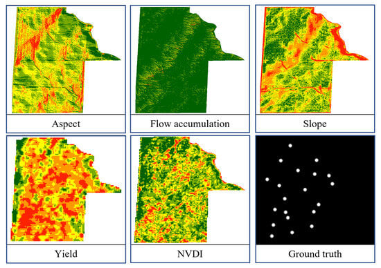
Figure 1.
A set of input and ground-truth images used for training and testing, corresponding to the characteristics and soil sampling locations in a field.
1.3. Contributions
This study underscores the critical need for innovative approaches in soil sampling mapping, particularly given the challenges encountered with existing models when applied to our dataset. Initial experimentation in our earlier work [14] with the Unet model revealed its inadequacy in effectively capturing the intricate features present in soil imagery data. Furthermore, while DeepLabv3 and FCN are established segmentation models, their performance on the soil dataset for soil sampling site selection fell short of expectations, as shown in Section 5.
Novelty: Recognizing the limitations of these conventional approaches, we have devised a novel strategy centered on building a dual deep learning architecture composed of a refiner and a selector. The refiner is designed to extract finer features from the input soil data. The selector analyzes the refined features to select the optimal locations for soil sampling matching the ground truth. The fusion of these dual components is enabled by a set of delicately designed bridge layers. The resultant segmentation models, our proposed models, UDL and UFN, exhibit remarkable improvements in accuracy and precision compared to state-of-the-art models.
The key scientific contributions of our work include the following:
- We develop a dual deep learning architecture capable of analyzing unbalanced soil mapping data and achieving better performance compared to existing methods.
- The models excel in handling multi-spectral images and generating highly efficient soil sampling maps.
- Our new soil sampling tools outperform existing methods.
- This work lays the foundation for integrating traditional and modern soil sampling methods.
The rest of this paper is organized as follows. Section 2 describes the dataset and data pre-processing. Section 3 elaborates on the methodologies of deep learning algorithms underlying the soil sampling tool. In addition, the algorithmic operation of the models is depicted, including the process of acquiring landscape attributes (aspect, flow accumulation, slope, yield, and Normalized Difference Vegetation Index), extracting patterns from these attributes, and generating optimal soil sampling locations. The model training and the metrics for evaluating the performance of the models are explained in Section 4. Section 5 discusses the results and compares the performance of the models. Finally, Section 6 provides some concluding remarks about this work.
2. Data Processing
2.1. Data Acquisition
The soil sampling dataset was gathered in Aurora and Davison counties, South Dakota, USA. In this work, the soil sampling dataset, named the 20s-Soil dataset, was collected on twenty homogeneous fields for training and testing our deep learning models. These fields were carefully selected to ensure homogeneity, with the same crop cultivated across all areas. The Digital Elevation Model (DEM) of each field was recorded from the LiDAR (Light Detection and Ranging) data, with each field ranging from 150 to 200 hectares and a spatial resolution of 10 m.
The 20s-Soil is a challenging dataset, where the input is a stack of multi-spectral images, and the ground truth is a highly unbalanced binary image. The ratio of black pixels (background) to white pixels (soil sampling sites) in the ground truth image is approximately 146:1. Specifically, an input is a set of five images, each representing a different attribute: aspect, flow accumulation, slope, yield, and Normalized Difference Vegetation Index (NDVI). Slope, aspect, and flow accumulation data were obtained from the DEMs using ArcMap (Esri®, ArcGIS, ArcMap 10.8). Additionally, NDVI values for each field were acquired through Sentinel 2A imagery downloaded from the Copernicus Open Hub, with a resolution of 10 m [43]. Furthermore, yield data were obtained through Field View Plus (Climate® Corporation, San Francisco, CA, USA). From this dataset, we conducted a multi-year yield average analysis using the SMS Ag software (https://www.agleader.com/farm-management/sms-software/ Ag Leader®, SMS Advanced). The yield data from 2018 to 2021, obtained from corn fields, were imported into the software. The software then provided the average yield for those years. The impact of terrain attributes such as slope and aspect, as well as hydrological attributes like flow accumulation, is considered a key factor for soil sampling practices. Typically, slope refers to the steepness or gradient of the terrain at a particular location. It is typically calculated by determining the rate of change in elevation over a given distance. Aspect describes the direction that a slope faces. Flow accumulation represents the accumulated flow of water at each cell in the DEM. It is used to identify drainage patterns and estimate the amount of water that will flow through a specific location [44].
In addition, the data layers cover 20 fields ranging from 150 to 200 hectares, resulting in an average size of 800 pixels by 1100 pixels. Figure 1 shows a set of input and ground-truth images, corresponding to the characteristics and soil sampling locations in a field. This paper focuses on developing a deep learning model capable of refining landscape data and extracting the optimal locations for soil sampling in a given field. In the context of our study, refinement encompasses identifying patterns in data, extracting important features, and improving data interpretability. The model is capable of processing a stack of five images (aspect, flow accumulation, slope, yield, and NDVI). It then learns by adjusting its internal parameters during the training process with ground-truth data to extract soil sampling locations (white pixels), as illustrated in Figure 1.
2.2. Data Augmentation
In order to make the data uniform and increase the number of samples for training and testing, we applied augmentation techniques. Initially, square images were cropped from the center of the input image, each with varying sizes. Subsequently, the cropped images were resized to dimensions of 572 × 572. Lastly, random rotations were applied to the resized images to generate additional data. It is important to note that when applying augmentation techniques to a set of input attributes, including aspect, slope, flow accumulation, yield, and NVDI, we stacked all attributes on top of each other. This means that during data augmentation, all input attributes within a set were rotated in the same manner and direction. We selected these augmentation methods due to their simplicity and computational efficiency.
The total dataset was subdivided into three sets: a training set comprising 2720 samples, a validation set with 340 samples, and a testing set consisting of 340 samples. Figure 2 illustrates the final augmented data of an image after random rotations.
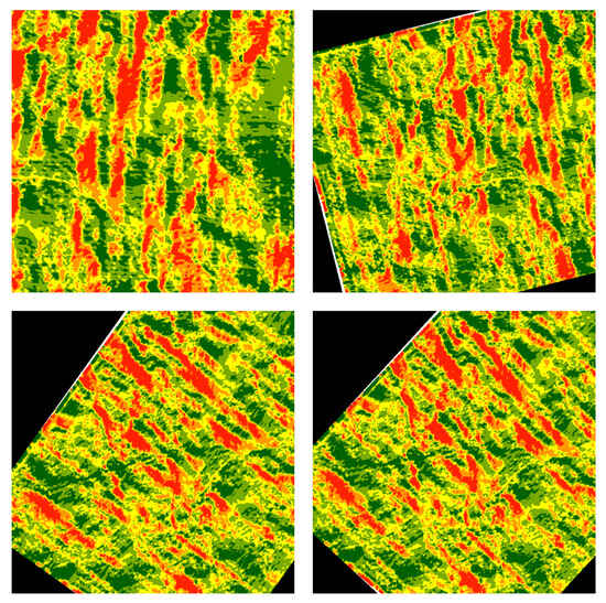
Figure 2.
Applying the random rotation technique on the resized images.
3. Methodology
3.1. Refiner: Extracting Fine Features by Leveraging an Encoder–Decoder Architecture
The refiner takes in a set of input images, including the aspect, flow accumulation, slope, yield, and NVDI attributes from a field. Each image represents a landscape attribute, as mentioned in Section 2.1. In particular, we designed the refiner based on an encoder–decoder architecture, inspired by Unet [37], to extract patterns from these inputs, producing feature maps as bridge layers B. Sequentially, these bridge layers B are fed into the selector’s backbone.
3.1.1. Encoder
The encoder consists of four building blocks, each composed of a basic block followed by a max-pooling function, as illustrated in Figure 3. The encoder allows the model to effectively reduce the input image’s dimensions and increase the number of feature maps. This structure enables the model to capture and retain hierarchical features at different scales.
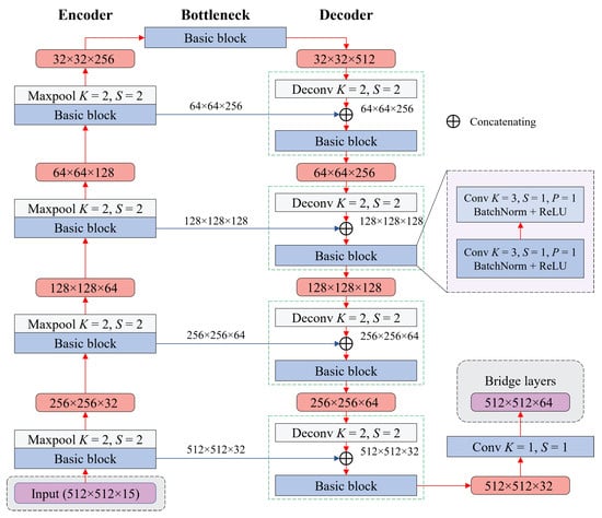
Figure 3.
Using an encoder–decoder model to extract the bridge layer from input images.
A single basic block includes two convolutional neural networks (CNNs) [25], followed by a batch normalization function [45] and a rectified linear unit (ReLU) activation function [46]. The structure of the basic block can be written as:
where and are the intermediate and final features of every basic block, respectively. , , and are the input, hidden, and output layers, respectively. After passing through the basic block, the resolution of the input image decreases while the number of features increases.
In particular, the output dimensions (H, W, C) of an input dataset, corresponding to the height, width, and number of channels (features), respectively, are computed after passing through a convolution, as follows:
where K, S, and P are the kernel, stride, and padding sizes, respectively. In all basic blocks, the values of K, S, and P are 3, 1, and 1, respectively, so the output dimensions of the convolution are the same as the inputs.
The output features are then passed through a max-pooling function with and , expressed as
thereby reducing the feature dimensions. Typically, the max-pooling function takes the maximum value of the given matrix (2 × 2), which reduces the dimensions two times. In addition, the numbers of output features after passing through four encoder blocks are 32, 64, 128, and 256, respectively.
3.1.2. Decoder
Unlike the encoder, the decoder consists of four building blocks, each of which comprises a basic block preceded by a deconvolution neural network (DCNN). The DCNN first upscales the input features and then concatenates them with the corresponding features from the encoder using skip connections. Typically, these skip connections allow information from the encoder to skip the subsequent operations and directly reach the decoder. The output dimensions of the input features after passing through the DCNN are calculated as:
where K, S, and P denote the kernel, stride, and padding sizes, respectively, similar to the CNN.
Sequentially, the concatenated features are fed into the basic block, extracting recovered features. This process is repeated for every decoder block. In the decoder, all DCNNs are designed to have K, S, and P are 2, 2, and 0, respectively, so the output dimensions are upscaled two times compared to the inputs. In addition, the numbers of output features are 256, 128, 64, and 32, respectively.
At the end of the decoder, we apply another convolution, with K = 1 and S = 1, to obtain the bridge layers B. These layers serve as inputs for the DeepLabv3 and FCN models. In addition, the resolutions of the bridge layers () are the same as the input images, and the number of bridge layers is 64.
3.2. Selector
The selector comprises a backbone and an output head. Fine features are first extracted by the refiner network, as described in the last section. The selector then establishes further relationships between features using a residual neural network backbone, grounded in the ResNet structure [47]. After that, it fuses the processed features and generates a prediction map. The rest of this section discusses the operation of these networks.
3.2.1. Selector Backbone
Figure 4 shows the architecture of the selector backbone constructed with atrous convolution neural networks (ACNNs), where R represents the number of backbone blocks. There are five main blocks in the network, including the pre-processing block and Blocks 1–4. These blocks serve as extractors, further extracting features from the bridge layers hierarchically. After passing through these blocks, the dimensions of the bridge layers decrease while the number of features increases.
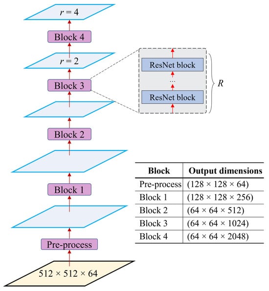
Figure 4.
The selector structure and the output dimensions of each block. Blocks 1 to 4 consist of a number (R) of ResNet blocks. In this context, when r = 1, it represents the outputs from the standard CNNs, whereas 1 indicates the outputs from the ACNNs.
In the pre-processing block, the bridge layers B are processed using a CNN , with K = 7, S = 2, and P = 2. This CNN is followed by a BatchNorm function [45] and a ReLU activation function [46]. The BatchNorm function normalizes the input of each layer by subtracting the mean and dividing by the standard deviation of the mini-batch of data. This centers the data around zero and scales them to have unit variance, ensuring that the activations in a neural network layer have a consistent and stable distribution during training. The pre-processing block is formulated as:
Again, represents the output features of the step, and and represent the number of input and output layers of this block, respectively. Sequentially, these features are passed into a max-pooling function with K = 2 and S = 2. As a result, the input’s dimension is reduced by a factor of through a sequence of CNN and max-pooling operations following the pre-processing block, resulting in a size of .
Blocks 1–4 consist of a number of ResNet blocks, whose architecture is shown in Figure 5. A single ResNet block consists of three CNN layers, where the first two layers are followed by a BatchNorm function and the third layer is followed by a BatchNorm function and a ReLU activation function. At the end of the third layer, the features are added to the input features to create the output layers. This connection is a simple element-wise addition, which allows the network to learn residual features instead of direct features. Therefore, these connections help the network avoid vanishing gradients during training.
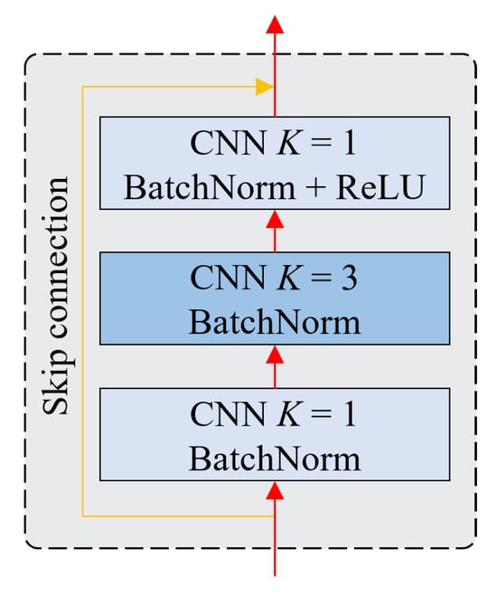
Figure 5.
The structure of a ResNet block.
In addition to the ResNet block, ACNNs are applied in Blocks 3 and 4 with an atrous rate r of 2 and 4, respectively, as shown in Figure 4. The ACNNs involve introducing gaps or “holes” in the traditional CNNs, thereby resulting in a larger receptive field without increasing the number of parameters, as visualized in Figure 6. The atrous rate r represents the empty spaces between the elements, and we can adjust this rate to capture different scale context information.
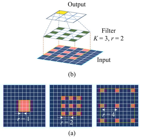
Figure 6.
(a) Construction of an atrous CNN, where r is the atrous or dilation rate. (b) Atrous CNN operation in the network with r = 2, and kernel size .
In this work, we employed ResNet50 and ResNet101 in the backbone to extract features. The difference between these neural networks is the number of ResNet blocks (R). For ResNet50, the number of ResNet blocks R in Blocks 1, 2, 3, and 4 is 3, 4, 6, and 3, respectively. For ResNet101, these numbers are 3, 4, 23, and 3, respectively. Given the bridge layers, B, the output dimensions of the features after passing through the ResNet blocks are (), (), (), (), and (), respectively.
3.2.2. Fuser
The resulting features of the backbone are fed into the fuser, a series of CNNs, where the features are further processed and fused to create the final prediction map. The output features from the network are processed by an atrous spatial pyramid pooling (ASPP) and a global average pooling (GAP) module operating in parallel, as shown in Figure 7. The idea behind the ASPP is to apply multiple convolutional filters with different atrous rates to the same input feature, which enables the model to capture information at varying spatial resolutions. The ASPP consists of a convolution (K = 1) and three (K = 3) convolutions with atrous rates of r = 12, 24, and 36. Following these convolutions are a BatchNorm function and a ReLU activation function , formulated as
where represents the output features of the backbone and is the output of the ith atrous spatial pyramid pooling module.
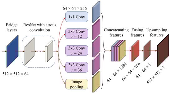
Figure 7.
The selector’s pipeline: The process of extracting features from bridge layers to produce the soil sampling prediction map.
Beyond ASPP, GAP is applied on top of the same output features from the backbone. Unlike max-pooling, GAP computes the average value of each channel across the entire spatial extent of the input feature map. It is used as a method to reduce the spatial dimensions of feature maps while retaining important information about the presence of different features in the image. In addition, the GAP module is followed by a BatchNorm function and a ReLU activation function , described similarly to the ASPP module in Equation (6).
The output features () from the ASPP and GAP modules are concatenated and then fused together using another convolution. As a result, the output dimensions after fusing are , and this step is formulated as
To obtain the prediction map, these fused features F are processed by a convolution followed by a BatchNorm function and a ReLU activation function before passing into a convolution. This process is described as
where M is the prediction mask with dimensions of (). Finally, the prediction mask is upscaled to match the input image using the linear interpolation function. This variant of the deep learning architecture is referred to as UDL, whose procedure is summarized in Algorithm 1. The next section describes the second variant.
| Algorithm 1 Pseudo-code explaining UDL’s algorithm |
|
3.2.3. Output Head
In addition to the UDL framework discussed above, we have also developed another variant of the deep learning architecture with an output head, called UFN. Both UDL and UFN share the same refiner and backbone; the difference is the output head. Specifically, the architecture of UFN is shown in Figure 8, while that of UDL is depicted in Figure 7.
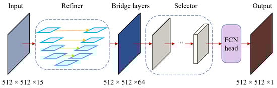
Figure 8.
UFN architecture.
In the UFN model, the output from the backbone is fed into the FCN head to produce predictions. First, the features are processed using a convolution , followed by a BatchNorm function and a ReLU activation function . Then, another convolution is applied on top of the processed features to create a prediction map, as described in Equation (8).
To match the input dimension, the prediction map is upscaled using the linear interpolation function. Specifically, the original dimensions of the bridge layers B () become after passing through the backbone. Then, the FCN head adopts these features and extracts a prediction known as a binary image (). As a result, this prediction is upscaled to to match the input dimensions. The process is described in detail by the pseudo-code in Algorithm 2.
| Algorithm 2 Pseudo-code explaining the soil sampling tool with the UFN model |
|
4. Experiment and Evaluations
4.1. Model Training
The innovative dual deep learning architectures, UDL described in Section 3.2.2 and UFN described in Section 3.2.3, were implemented using the PyTorch framework and Torchvision library. To train our model, we utilized a high-performance computing facility named AI.Panther, equipped with A100 SXM4 GPUs, hosted at the Florida Institute of Technology.
As mentioned in Section 3, the final predictions are binary images. Therefore, we used the binary cross-entropy (BCE) loss as an objective function during the training process. The BCE loss measures the difference between the predicted probabilities and the true labels of every pixel in the ground truth. For a pair consisting of a prediction M and a ground truth Y, the average loss is defined as follows:
where Q is the number of pixels in the prediction or ground truth, q is the index of the pixel, and represents the parameters in our deep learning models, iteratively adjusted to minimize the loss.
Throughout the training process, the stochastic gradient descent (SGD) algorithm was used to find the optimal values for the model’s parameters that minimized the loss between the prediction and ground truth. The gradients indicated the direction in which the parameters should be updated to reduce the loss. During this step, SGD is updated with a learning rate of , a hyperparameter used to control the step size for the parameter update. In addition, we used weight decay regularization of in combination with a momentum of to prevent overfitting. The training procedure involved feeding data into models for multiple epochs, where one epoch was completed when the entire dataset was passed into the model. To optimize the training process with respect to available computational resources, we divided the total training dataset N into multiple batches, , for an epoch. Therefore, the model needed to iterate I times to complete an epoch, with the number of iterations calculated as
4.2. Evaluation Metrics
The performance of the proposed combined models was assessed using standard metrics for binary segmentation, including the mean Intersection over Union (mIoU) and mean Dice Coefficient (mDC). Before we computed these metrics, we applied the thresholding technique to the final prediction with a threshold value of 190. In doing so, all pixel values less than 190 were converted to 0 (black), and the others were converted to 1 (white). To facilitate the metric calculation, we provide the following definitions:
- True positive (TP) is the total number of white pixels that the model correctly predicted compared to the white pixels on the ground truth.
- True negative (TN) is the total number of black pixels that the model correctly predicted compared to the black pixels on the ground truth.
- False positive (FP) is the total number of white pixels that the model predicted to overlap with the black pixels on the ground truth.
- False negative (FN) is the total number of black pixels that the model predicted to overlap with the white pixels in the ground truth.
The mIoU, the mean overlap of the predictions and ground truths over the total N images, is computed as follows:
The mDC, the mean similarity between the predictions generated by the model and the ground truths, is defined as follows:
5. Results and Discussion
In this section, we report the efficacy of our proposed dual deep learning models by comparing their performance with state-of-the-art segmentation models. In addition, we tested the performance of our models with different numbers of layers in the backbone, i.e., UDL50 for UDL with 50 backbone layers and UDL101 for UDL with 101 backbone layers. Similarly, UFN50 and UFN101 stand for UFN with 50 and 101 backbone layers, respectively. These models were trained and compared with their counterparts, as well as several existing state-of-the-art methods.
5.1. Soil Sampling Tool Based on UDL
The training process of the UDL model is shown in Figure 9. All the models converged after 100 epochs, with the models with a 101-layer backbone showing lower losses compared to those with a 50-layer backbone. Moreover, on the validation set, after 1000 epochs, UDL50 and UDL101 achieved loss values of 0.011 and 0.007, respectively, whereas DeepLabv3-Res50 and DeepLabv3-Res101, two state-of-the-art models, recorded loss values of 0.012 and 0.009, respectively. Our dual deep learning models exhibited lower loss values on the validation dataset compared to the SOTA models, with the UDL101 model exhibiting the lowest training loss.
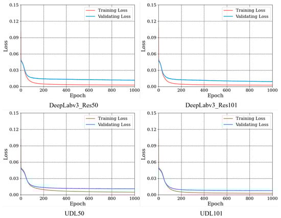
Figure 9.
The training and evaluation losses of the UDL and DeepLabv3 models during the training process.
To gain more a comprehensive insight into the models, all models were saved at every 10 epochs during the training. These saved weights were loaded and implemented on the training, validation, and test datasets to compare the performance of the models. We used the metrics mentioned in Section 4.2 (mIoU and mDC) to evaluate the models’ performance. If the metric measurements on both the validation and testing sets declined over time, it indicated that the model was potentially overtrained. Furthermore, if the models’ performance metrics consistently improved with an increasing number of epochs, the training could be extended for more epochs.
On the test set, the highest mDC values for the DeepLabv3-Res50, DeepLabv3-Res101, UDL50, and UDL101 models were 56.28%, 63.75%, 66.82%, and 73.74%, respectively, whereas the mIoU values were 41.44%, 49.24%, 51.96%, and 60.68%, respectively. Thus, we chose the best models to make predictions on the test dataset, as shown in Figure 10. It is evident from the figure that the UDL model exhibited higher accuracy in predicting both the foreground and background compared to the other models. Additionally, the performance metrics of the top-performing models were computed, as shown in Table 1.
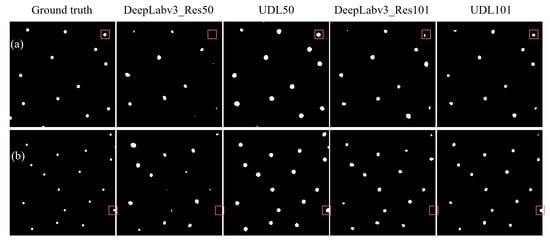
Figure 10.
Comparison of qualitative results between UDL and DeepLabv3. The predicted soil sampling maps on different fields (a,b) with respect to the best weights of different models. The square boxes highlight the differences between the predictions of the models.

Table 1.
Quantitative comparison of UDL and DeepLabv3 using the evaluation metrics.
5.2. Soil Sampling Tool Based on UFN
For the proposed UFN models, we conducted training and compared their performance with that of their counterparts. The training and validation losses during the training of the two models are shown in Figure 11. All models converged after around 100 epochs, and again, the evaluation losses of our models, UFNs, were lower than those of their counterparts. Specifically, after 1000 epochs of training, the loss values for UFN50 and UFN101 were 0.011 and 0.008, respectively, whereas the loss values for FCN-Res50 and FCN-Res101 were 0.013 and 0.012, respectively.
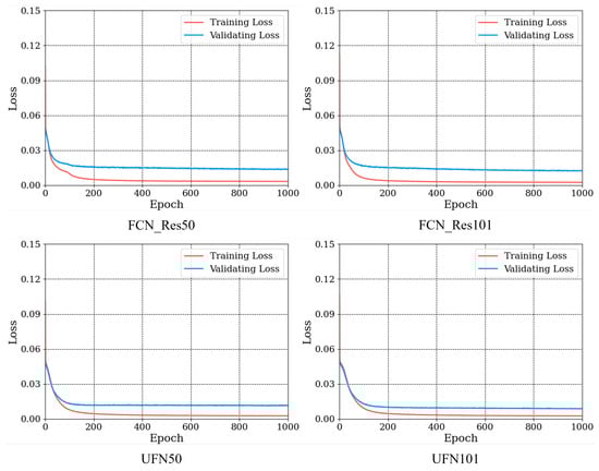
Figure 11.
Losses for the UFN models during the training process.
For the UFN and FCN models, we also trained the models up to 1000 epochs and saved the weights of the models every ten epochs. The saved models were used to perform predictions on the test dataset, and their performance was compared. The prediction maps for soil sampling are depicted in Figure 12, and a detailed summary of their performance metrics can be found in Table 2.
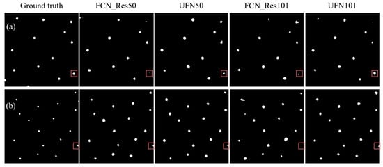
Figure 12.
Comparison of qualitative results between UFN and FCN. In the subfigures, black represents the background, and white dots indicate soil sampling locations. Square boxes highlight differences between the models’ predictions.
Table 2.
Quantitative comparison of UFN and FCN using the evaluation metrics. In the table, Val. stands for the validation dataset.
Intuitively, the predictions from the combined models were more accurate compared to the predictions from their original counterparts. If we take a look at the size and shape of the predictions, it is evident that the UFN101 model produced soil sampling maps that closely resembled the ground truths. The square boxes in Figure 12 highlight the differences between the predictions generated by these models.
In terms of quantitative comparison, the highest mDC values for the FCN-Res50, FCN-Res101, UFN50, and UFN101 models on the test dataset were 65.97%, 58.88%, 68.62%, and 69.12%, respectively, whereas the mIoU values were 52.34%, 44.32%, 55.42%, and 55.45%, respectively. It is evident from the results that our innovative UFN models consistently outperformed the state-of-the-art FCN models. Notably, UFN101 exhibited the best performance among all models on the test dataset.
5.3. Comparison of Soil Sampling Tools
In this section, we compare the performance of our proposed models with the latest machine learning-based soil sampling tool [14]. The quantitative comparison is shown in Table 3. It is evident that the UDL101 not only outperformed the established model but also exhibited superior capabilities compared to the Transformer-based model from our previous investigation. This observation leads us to conclude that our proposed model demonstrates substantial promise for soil sampling segmentation.
Table 3.
Quantitative comparison of soil sampling tools using the evaluation metrics. In the table, Val. stands for the validation dataset.
6. Conclusions
In this paper, we proposed refiner–selector models as the backbones of soil sampling tools capable of generating sampling locations. The prediction tool in this work can handle a challenging dataset, where the input consists of a stack of multi-spectral images, and the output is a highly unbalanced binary image. Here, each input image represents a landscape attribute, and the output image is an optimal soil sampling map.
Additionally, the UDL and UFN models were proposed for soil sampling map prediction. These models consist of a refiner network and an output head. The refiner is designed to produce bridge layers, which are then fed into Resnet and the output head. For consistency, we used ResNet50 and ResNet101 as the backbones of the UDL and UFN models.
For experimental validation, we trained the UDL and UFN models and then compared them with their counterparts. The experimental results indicate that the proposed models outperformed the established segmentation models on the soil sampling dataset (Soil-20s). In addition, the performance of the UDL models was better than that of the UFN models, and the combined models with the ResNet101 backbone produced better results. During the experiments, the best model was UDL101, which achieved an mIoU of 60.82% and an mDC of 73.74% on the test dataset. The values of these metrics for the DeepLabv3-Res101 and FCN-Res101 models were 49.24% and 63.75%, and 44.32% and 58.88%, respectively.
The results of this study demonstrate that using fine feature maps is better for handling challenging soil datasets compared to raw input images. In the soil sampling dataset, the accuracy of the soil sampling tool increased by 6.1% and 3.18% in terms of the mIoU and mDC metrics, respectively, when using UDL101. This tool enables technicians and farmers to select samples more accurately, thus furthering our comprehension of soil health.
With improvements to the new soil sampling framework, the next step of this research is to develop an efficient automatic tool or mobile app that can help farmers and producers in implementing the tool on their farms. Building a larger dataset that can be used globally will also be considered in our future research. We plan to explore the integration of time-series satellite imagery from diverse sources, such as EnMAP, Sentinel-1, Sentinel-2, LandSat, and MODIS, to capture temporal variations in vegetation indices and soil properties over multiple seasons. Additionally, we will investigate advanced data augmentation techniques beyond traditional techniques, including the use of generative models such as GANs and diffusion models. The feasibility of integrating soil analysis data into our study will also be explored through further collaboration with soil scientists and agronomists.
Author Contributions
T.-H.P.: Conceptualization, investigation, methodology, formal analysis, validation, visualization, writing—original draft. K.-D.N.: Conceptualization, methodology, formal analysis, writing—review and editing, funding acquisition. All authors have read and agreed to the published version of the manuscript.
Funding
This research was funded by grants #2021-67022-38910 and #2022-67021-38911 from the USDA National Institute of Food and Agriculture. APC was funded by these grants and the Open Access Subvention Fund from Evans Library at Florida Institute of Technology.
Data Availability Statement
The data that support the findings of this study are available from the corresponding author upon reasonable request.
Conflicts of Interest
The authors declare no conflict of interest.
References
- Rowell, D.L. Soil Science: Methods & Applications; Routledge: Oxfordshire, UK, 2014. [Google Scholar]
- Brus, D.; Kempen, B.; Heuvelink, G. Sampling for validation of digital soil maps. Eur. J. Soil Sci. 2011, 62, 394–407. [Google Scholar] [CrossRef]
- Dane, J.H.; Topp, C.G. Methods of Soil Analysis, Part 4: Physical Methods; John Wiley & Sons: Hoboken, NJ, USA, 2020; Volume 20. [Google Scholar]
- Hengl, T.; Leenaars, J.G.; Shepherd, K.D.; Walsh, M.G.; Heuvelink, G.B.; Mamo, T.; Tilahun, H.; Berkhout, E.; Cooper, M.; Fegraus, E.; et al. Soil nutrient maps of Sub-Saharan Africa: Assessment of soil nutrient content at 250 m spatial resolution using machine learning. Nutr. Cycl. Agroecosyst. 2017, 109, 77–102. [Google Scholar] [CrossRef]
- Poggio, L.; De Sousa, L.M.; Batjes, N.H.; Heuvelink, G.; Kempen, B.; Ribeiro, E.; Rossiter, D. SoilGrids 2.0: Producing soil information for the globe with quantified spatial uncertainty. Soil 2021, 7, 217–240. [Google Scholar] [CrossRef]
- Hengl, T.; Miller, M.A.; Križan, J.; Shepherd, K.D.; Sila, A.; Kilibarda, M.; Antonijević, O.; Glušica, L.; Dobermann, A.; Haefele, S.M.; et al. African soil properties and nutrients mapped at 30 m spatial resolution using two-scale ensemble machine learning. Sci. Rep. 2021, 11, 6130. [Google Scholar] [CrossRef]
- John, K.; Abraham Isong, I.; Michael Kebonye, N.; Okon Ayito, E.; Chapman Agyeman, P.; Marcus Afu, S. Using machine learning algorithms to estimate soil organic carbon variability with environmental variables and soil nutrient indicators in an alluvial soil. Land 2020, 9, 487. [Google Scholar] [CrossRef]
- Hassani, A.; Azapagic, A.; Shokri, N. Predicting long-term dynamics of soil salinity and sodicity on a global scale. Proc. Natl. Acad. Sci. USA 2020, 117, 33017–33027. [Google Scholar] [CrossRef]
- Batjes, N.H.; Ribeiro, E.; Van Oostrum, A. Standardised soil profile data to support global mapping and modelling (WoSIS snapshot 2019). Earth Syst. Sci. Data 2020, 12, 299–320. [Google Scholar] [CrossRef]
- Folorunso, O.; Ojo, O.; Busari, M.; Adebayo, M.; Joshua, A.; Folorunso, D.; Ugwunna, C.O.; Olabanjo, O.; Olabanjo, O. Exploring machine learning models for soil nutrient properties prediction: A systematic review. Big Data Cogn. Comput. 2023, 7, 113. [Google Scholar] [CrossRef]
- Pham, V.; Weindorf, D.C.; Dang, T. Soil profile analysis using interactive visualizations, machine learning, and deep learning. Comput. Electron. Agric. 2021, 191, 106539. [Google Scholar] [CrossRef]
- Pyo, J.; Hong, S.M.; Kwon, Y.S.; Kim, M.S.; Cho, K.H. Estimation of heavy metals using deep neural network with visible and infrared spectroscopy of soil. Sci. Total Environ. 2020, 741, 140162. [Google Scholar] [CrossRef]
- Jia, X.; O’Connor, D.; Shi, Z.; Hou, D. VIRS based detection in combination with machine learning for mapping soil pollution. Environ. Pollut. 2021, 268, 115845. [Google Scholar] [CrossRef]
- Pham, T.H.; Acharya, P.; Bachina, S.; Osterloh, K.; Nguyen, K.D. Deep-learning framework for optimal selection of soil sampling sites. Comput. Electron. Agric. 2024, 217, 108650. [Google Scholar] [CrossRef]
- Ozbayoglu, A.M.; Gudelek, M.U.; Sezer, O.B. Deep learning for financial applications: A survey. Appl. Soft Comput. 2020, 93, 106384. [Google Scholar] [CrossRef]
- Pham, T.H.; Li, X.; Nguyen, K.D. SeUNet-Trans: A Simple yet Effective UNet-Transformer Model for Medical Image Segmentation. arXiv 2023, arXiv:2310.09998. [Google Scholar]
- Bhardwaj, P.; Gupta, P.; Panwar, H.; Siddiqui, M.K.; Morales-Menendez, R.; Bhaik, A. Application of deep learning on student engagement in e-learning environments. Comput. Electr. Eng. 2021, 93, 107277. [Google Scholar] [CrossRef]
- Voulodimos, A.; Doulamis, N.; Doulamis, A.; Protopapadakis, E. Deep learning for computer vision: A brief review. Comput. Intell. Neurosci. 2018, 2018, 7068349. [Google Scholar] [CrossRef]
- Hassaballah, M.; Awad, A.I. Deep Learning in Computer Vision: Principles and Applications; CRC Press: Boca Raton, FL, USA, 2020. [Google Scholar]
- Jia, W.; Tian, Y.; Luo, R.; Zhang, Z.; Lian, J.; Zheng, Y. Detection and segmentation of overlapped fruits based on optimized mask R-CNN application in apple harvesting robot. Comput. Electron. Agric. 2020, 172, 105380. [Google Scholar] [CrossRef]
- Kuznetsova, A.; Maleva, T.; Soloviev, V. Using YOLOv3 algorithm with pre-and post-processing for apple detection in fruit-harvesting robot. Agronomy 2020, 10, 1016. [Google Scholar] [CrossRef]
- Acharya, P.; Burgers, T.; Nguyen, K.D. Ai-enabled droplet detection and tracking for agricultural spraying systems. Comput. Electron. Agric. 2022, 202, 107325. [Google Scholar] [CrossRef]
- Acharya, P.; Burgers, T.; Nguyen, K.D. A deep-learning framework for spray pattern segmentation and estimation in agricultural spraying systems. Sci. Rep. 2023, 13, 7545. [Google Scholar]
- Pham, T.H.; Nguyen, K.D. Enhanced Droplet Analysis Using Generative Adversarial Networks. arXiv 2024, arXiv:2402.15909. [Google Scholar]
- LeCun, Y.; Bengio, Y. Convolutional networks for images, speech, and time series. Handb. Brain Theory Neural Netw. 1995, 3361, 1995. [Google Scholar]
- LeCun, Y.; Bottou, L.; Bengio, Y.; Haffner, P. Gradient-based learning applied to document recognition. Proc. IEEE 1998, 86, 2278–2324. [Google Scholar] [CrossRef]
- Dosovitskiy, A.; Beyer, L.; Kolesnikov, A.; Weissenborn, D.; Zhai, X.; Unterthiner, T.; Dehghani, M.; Minderer, M.; Heigold, G.; Gelly, S.; et al. An image is worth 16 × 16 words: Transformers for image recognition at scale. arXiv 2020, arXiv:2010.11929. [Google Scholar]
- Vaswani, A.; Shazeer, N.; Parmar, N.; Uszkoreit, J.; Jones, L.; Gomez, A.N.; Kaiser, Ł.; Polosukhin, I. Attention is all you need. Adv. Neural Inf. Process. Syst. 2017, 30. [Google Scholar]
- Girshick, R.; Donahue, J.; Darrell, T.; Malik, J. Rich feature hierarchies for accurate object detection and semantic segmentation. In Proceedings of the IEEE Conference on Computer Vision and Pattern Recognition, Columbus, OH, USA, 23–28 June 2014; pp. 580–587. [Google Scholar]
- Ren, S.; He, K.; Girshick, R.; Sun, J. Faster r-cnn: Towards real-time object detection with region proposal networks. Adv. Neural Inf. Process. Syst. 2015, 28. [Google Scholar] [CrossRef] [PubMed]
- Redmon, J.; Divvala, S.; Girshick, R.; Farhadi, A. You only look once: Unified, real-time object detection. In Proceedings of the IEEE Conference on Computer Vision and Pattern Recognition, Las Vegas, NV, USA, 27–30 June 2016; pp. 779–788. [Google Scholar]
- Liu, W.; Anguelov, D.; Erhan, D.; Szegedy, C.; Reed, S.; Fu, C.Y.; Berg, A.C. Ssd: Single shot multibox detector. In Proceedings of the Computer Vision–ECCV 2016: 14th European Conference, Amsterdam, The Netherlands, 11–14 October 2016; Proceedings, Part I 14. Springer: Berlin/Heidelberg, Germany, 2016; pp. 21–37. [Google Scholar]
- Carion, N.; Massa, F.; Synnaeve, G.; Usunier, N.; Kirillov, A.; Zagoruyko, S. End-to-end object detection with transformers. In Proceedings of the European Conference on Computer Vision, Glasgow, UK, 23–28 August 2020; pp. 213–229. [Google Scholar]
- Zhu, X.; Su, W.; Lu, L.; Li, B.; Wang, X.; Dai, J. Deformable detr: Deformable transformers for end-to-end object detection. arXiv 2020, arXiv:2010.04159. [Google Scholar]
- Havaei, M.; Davy, A.; Warde-Farley, D.; Biard, A.; Courville, A.; Bengio, Y.; Pal, C.; Jodoin, P.M.; Larochelle, H. Brain tumor segmentation with deep neural networks. Med. Image Anal. 2017, 35, 18–31. [Google Scholar] [CrossRef] [PubMed]
- Long, J.; Shelhamer, E.; Darrell, T. Fully convolutional networks for semantic segmentation. In Proceedings of the IEEE Conference on Computer Vision and Pattern Recognition, Boston, MA, USA, 7–12 June 2015; pp. 3431–3440. [Google Scholar]
- Ronneberger, O.; Fischer, P.; Brox, T. U-net: Convolutional networks for biomedical image segmentation. In Proceedings of the Medical Image Computing and Computer-Assisted Intervention–MICCAI 2015: 18th International Conference, Munich, Germany, 5–9 October 2015; Proceedings, Part III 18. Springer: Berlin/Heidelberg, Germany, 2015; pp. 234–241. [Google Scholar]
- He, K.; Gkioxari, G.; Dollár, P.; Girshick, R. Mask r-cnn. In Proceedings of the IEEE International Conference on Computer Vision, Venice, Italy, 22–29 October 2017; pp. 2961–2969. [Google Scholar]
- Chen, L.C.; Papandreou, G.; Schroff, F.; Adam, H. Rethinking atrous convolution for semantic image segmentation. arXiv 2017, arXiv:1706.05587. [Google Scholar]
- Xie, E.; Wang, W.; Yu, Z.; Anandkumar, A.; Alvarez, J.M.; Luo, P. SegFormer: Simple and efficient design for semantic segmentation with transformers. Adv. Neural Inf. Process. Syst. 2021, 34, 12077–12090. [Google Scholar]
- Jain, J.; Li, J.; Chiu, M.T.; Hassani, A.; Orlov, N.; Shi, H. Oneformer: One transformer to rule universal image segmentation. In Proceedings of the IEEE/CVF Conference on Computer Vision and Pattern Recognition, Vancouver, BC, Canada, 17–24 June 2023; pp. 2989–2998. [Google Scholar]
- Kirillov, A.; Mintun, E.; Ravi, N.; Mao, H.; Rolland, C.; Gustafson, L.; Xiao, T.; Whitehead, S.; Berg, A.C.; Lo, W.Y.; et al. Segment anything. arXiv 2023, arXiv:2304.02643. [Google Scholar]
- ESA. Copernicus Sentinel Data. 2023. Available online: https://search.asf.alaska.edu/#/ (accessed on 1 April 2023).
- Martz, L.W.; Garbrecht, J. Automated extraction of drainage network and watershed data from digital elevation models 1. Jawra J. Am. Water Resour. Assoc. 1993, 29, 901–908. [Google Scholar] [CrossRef]
- Ioffe, S.; Szegedy, C. Batch normalization: Accelerating deep network training by reducing internal covariate shift. In Proceedings of the International Conference on Machine Learning, Pmlr, Lille, France, 7–9 July 2015; pp. 448–456. [Google Scholar]
- Nair, V.; Hinton, G.E. Rectified linear units improve restricted boltzmann machines. In Proceedings of the 27th International Conference on Machine Learning (ICML-10), Haifa, Israel, 21–24 June 2010; pp. 807–814. [Google Scholar]
- He, K.; Zhang, X.; Ren, S.; Sun, J. Deep residual learning for image recognition. In Proceedings of the IEEE Conference on Computer Vision and Pattern Recognition, Las Vegas, NV, USA, 27–30 June 2016; pp. 770–778. [Google Scholar]
Disclaimer/Publisher’s Note: The statements, opinions and data contained in all publications are solely those of the individual author(s) and contributor(s) and not of MDPI and/or the editor(s). MDPI and/or the editor(s) disclaim responsibility for any injury to people or property resulting from any ideas, methods, instructions or products referred to in the content. |
© 2024 by the authors. Licensee MDPI, Basel, Switzerland. This article is an open access article distributed under the terms and conditions of the Creative Commons Attribution (CC BY) license (https://creativecommons.org/licenses/by/4.0/).