Autoencoder Feature Residuals for Network Intrusion Detection: One-Class Pretraining for Improved Performance ^†

Abstract

The proliferation of novel attacks and growing amounts of data has caused practitioners in the field of network intrusion detection to constantly work towards keeping up with this evolving adversarial landscape. Researchers have been seeking to harness deep learning techniques in efforts to detect zero-day attacks and allow network intrusion detection systems to more efficiently alert network operators. The technique outlined in this work uses a one-class training process to shape autoencoder feature residuals for the effective detection of network attacks. Compared to an original set of input features, we show that autoencoder feature residuals are a suitable replacement, and often perform at least as well as the original feature set. This quality allows autoencoder feature residuals to prevent the need for extensive feature engineering without reducing classification performance. Additionally, it is found that without generating new data compared to an original feature set, using autoencoder feature residuals often improves classifier performance. Practical side effects from using autoencoder feature residuals emerge by analyzing the potential data compression benefits they provide.

1. Introduction

The reliance on computer networks in our daily lives has grown in both magnitude and complexity in recent years [1]. The comparative growth in network attacks has brought network security to the forefront for many organizations [2]. To prevent the drastic consequences of network attacks, a network intrusion detection system (NIDS) alerts network operators when an attack is present. Researchers have recently focused their efforts to take advantage of deep learning techniques as a way to detect complex network attacks and improve the protection provided by a NIDS [2,3,4,5].

This article is an extended version of our paper published in the Proceedings of the 21st IEEE International Conference on Machine Learning and Applications (ICMLA), 2022 [6]. Here, we develop the use of autoencoder feature residuals to generate features for various neural network architectures including this extension of the technique to use sequential network data with recurrent neural network classifiers. Previously introduced work showed that this technique is effective for network intrusion detection when paired with traditional classifiers such as random forest and k-nearest neighbors [7]. What was not treated in that work, however, was the application of the technique in conjunction with neural network architectures, such as feedforward and recurrent neural networks, which are used in state-of-the-art research today. Here, we extend the literature by exploring the application of autoencoder feature residuals to several neural network architectures and assess their performance. In particular, we analyze performance using autoencoder feature residuals in combination with feedforward neural networks and various architectures of recurrent neural networks.

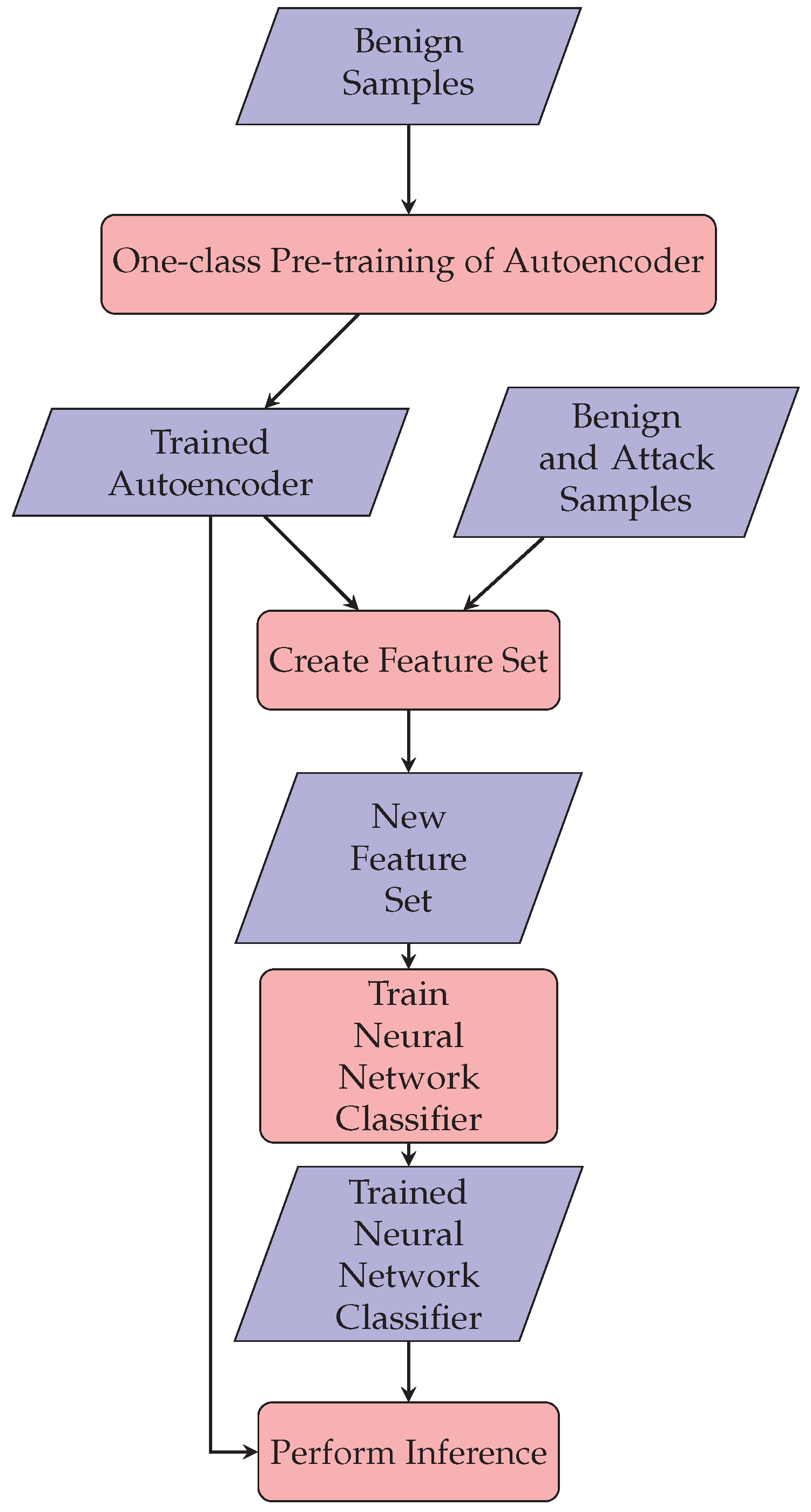
The process for generating and using autoencoder feature residuals can be summarized by a series of four steps, which are displayed in Figure 1. Taking only benign network flow samples, an autoencoder is trained. This trained autoencoder can then be provided with benign and attack network samples to construct a number of novel feature sets using autoencoder feature residuals. These feature sets then train a neural network such that it can effectively classify a given network sample as attack or benign. With both trained models in hand, we can then perform inference on novel samples. We show that autoencoder feature residuals perform as well as an original set of input features and have the potential to increase performance under certain conditions. Unlike most other works that use autoencoders for network intrusion detection, we do not rely on summary metrics such as mean-squared error when utilizing autoencoder reconstruction error [3,4,8]. By exploring this process, we have found that there is value in using the individual residuals of each feature. In addition, we show that using autoencoder feature residuals has benefits in terms of data compression, even in the cases where classification performance is not improved.

When using information theory as a guide, it is surprising that our technique performs as well as an original feature set. By strictly removing data from our original feature set, our comparable performance shows that the mutual information between features and labels used during training is preserved [9].

The main contributions of our work are as follows:

• We introduce the first application of using autoencoder feature residuals as input to a feedforward neural network classifier for network intrusion problems;
• We introduce the first application of using autoencoder feature residuals as input to recurrent neural network classifiers for network intrusion problems;
• We provide an analysis of the application of our technique across five benchmark datasets consisting of seven network intrusion scenarios, and two different encodings of the data;
• Using f1-score and p-values from the Kolmogorov–Smirnov test, we show that using autoencoder feature residuals, either in place of an original feature set or in combination with it, does no harm to classifier performance and has the potential to improve it;
• We identify the potential data compression benefits when using autoencoder feature residuals;
• We make our implemented code and data publicly available (https://github.com/WickedElm/feature_residuals_with_pretraining, accessed on 12 June 2023) for use by other researchers.

The remainder of this article is structured as follows. In Section 1, we discuss recent related works in network intrusion detection. Section 2 provides the reader with necessary background information associated with the work and outlines our methodology. Our results and their associated discussion are presented in Section 3. Finally, we conclude the article in Section 4.

Related Work

This work is rooted within several areas of research, including anomaly detection and deep learning, as well as their application to network intrusion detection. A key assumption of the work relies on the one-class pretraining step producing an autoencoder, which has difficulty reconstructing network attacks compared to benign network samples. This assumption is made by similar techniques, in that the residuals for attack samples will have more data in them; however, they often use an aggregate summary error metric in combination with a threshold [10]. Other techniques that utilize autoencoders in this space make use of the bottleneck layer for feature reduction/selection [10].

One recent work that utilizes this assumption introduces a method where the authors train an autoencoder to detect distributed denial-of-service attacks [11]. In their work, the authors focus on the industrial cyberphysical environment by using lightweight features as input to an autoencoder. Using only benign network flows during training, they are able to detect attack network flows using the autoencoder’s reconstruction mean-squared error compared to a threshold. Similarly, another recent work uses this same concept as part of a larger two-stage system to detect network attacks [12]. In the first stage of the system, the authors use a light gradient-boosting model to perform initial detection of network attacks. An autoencoder is used in the second stage to confirm that any network flows identified as benign also have a reconstruction mean-squared error that is below a threshold as a second check.

AIDA is a full NIDS introduced to detect network attacks [3]. The AIDA system uses a single autoencoder residual for each sample to augment their classifier input features. Similarly, a related work produces three additional features using a stacked sparse autoencoder [13]. First, a bottleneck layer of a single node is utilized as a feature. The authors then use two forms of the reconstruction error from the autoencoder, euclidean distance and cosine similarity, as the other two additional features. While these works share a similarity in concept to our work, we propose using the residual of each reconstructed feature as opposed to a summary metric.

Two systems are outlined that include an ensemble of autoencoders to detect network attacks in an unsupervised manner [4,8]. While these systems differ in their specific implementations, both use the root-mean-squared errors from reconstructions in the ensemble as their primary metric for detecting network attacks.

An emerging technique involves the use of triplet networks being formed by providing them with autoencoder reconstructions [14]. In one-class training, the two autoencoders are trained on benign and attack network data separately. The reconstructions of novel samples are provided to the triplet network to determine if it is attack or benign during inference. Another application of triplet networks involving the use of autoencoders augments this idea by providing the triplet network with the output of the encoder’s bottleneck layer [5].

Through an analysis of the effects of autoencoder bottleneck size on performance, one recent work uses a z-score threshold on the autoencoder reconstruction error [10]. Trained only on benign network data, it is shown that such a summary metric can be used for detecting network attacks.

It is common to see feedforward networks used to classify network attacks [15,16]. While some works use only a single feedforward layer as part of a larger model [17], others use a larger feedforward network as their main classifier [18]. A recent work that presents the IGRF-RFE feature selection method utilizes a multilayer perceptron to perform classification of netflow data using features derived from an ensemble feature selection and reduction method [19]. Increasing in popularity are works that use recurrent neural networks (RNNs) as part of their proposed methods [15,16]. In one interesting work, the HCRNNIDS method is introduced, which uses a combination of convolutional networks and a recurrent neural network together [20]. The convolutional network is intended to focus on local features in network flow data, while the recurrent network then focuses on using temporal features.

Another work making use of recurrent neural networks takes an ensemble consisting of an RNN, gated recurrent unit (GRU), and long short-term memory (LSTM) model in order to perform feature extraction on network flow data [21]. The various extracted features from the ensemble are then combined to be used with a downstream classifier. A similar method makes use of an autoencoder by extracting the bottleneck layer as features for input to a downstream RNN classifier [22].

Rather than using two separate models, other works combine model architectures, as was carried out for the DDoSNet model [23]. For this suggested NIDS, an autoencoder was constructed using recurrent layers. The bottleneck layer was then used to successfully classify distributed denial of service attacks using network flow data.

Among the few works that use autoencoder feature residuals, one that stands out details the DeepAID framework [24]. This proposed framework takes autoencoder feature residuals with the purpose of adding interpretability to deep learning-based anomaly detection systems. Unlike our work, however, DeepAID does not perform anomaly detection, and rather focuses on analyzing previously detected anomalies. Similar interpretability comes for free with our technique, as the feature residuals of attack samples with high magnitude identify the particular features that deviate the most from benign data.

Another work incorporates autoencoder feature residuals into a larger system focused on transfer learning [25]. The authors train an autoencoder on each device on a network and then use a global classifier to detect attacks from network data. The input to the global classifier are normalized autoencoder feature residuals. While the focus of that work is on their entire NIDS, we differentiate our work by explicitly exploring the use of autoencoder feature residuals and capturing their performance across multiple feature encodings in order to show their general applicability with several architectures of neural network classifiers.

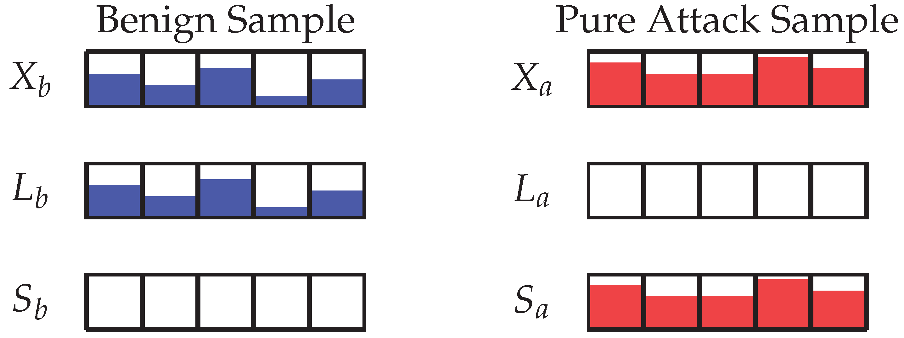
One of the main drawbacks for the related works discussed here is that by using an aggregate residual for detecting network attacks, it is possible for valuable information to be lost. This can be demonstrated with the synthetic example shown in Figure 2, where we have two clearly different network samples, one being benign and the other an attack. Previously discussed techniques that use mean-squared error [3,4,8,11] or some other aggregate metric [13] are destined to incorrectly classify one of these samples. When using our technique, however, we are still able to differentiate samples such as these by providing the structure of the samples to a downstream classifier, since the residual for each feature is preserved.

Broad overviews of network intrusion detection techniques can be found in a number of recent surveys of the area. Several, such as [2,15], cover both anomaly detection and deep learning techniques for network intrusion detection.

2. Materials and Methods

In this section, we review the information needed to generate autoencoder feature residuals. Autoencoder feature residuals are defined, and we walk through the methodology used to evaluate their performance compared to using an original feature set.

2.1. Autoencoders

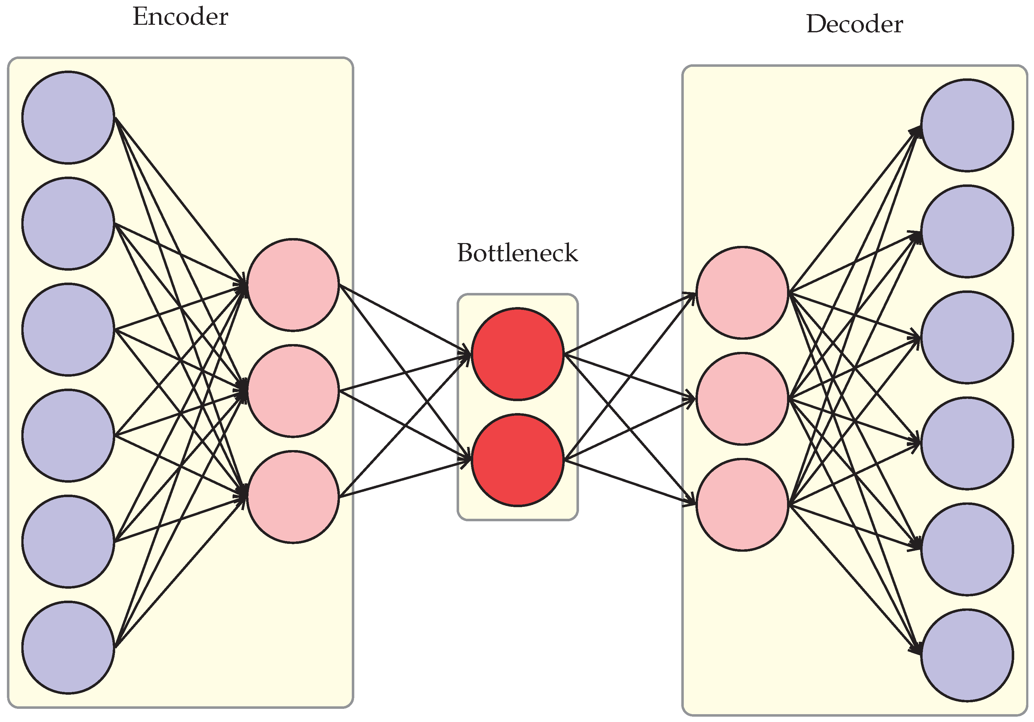
Autoencoders are a well-known form of neural network with properties that lend themselves to a number of useful applications such as data generation, feature selection and reduction, denoising, and anomaly detection [26]. The uniqueness of the autoencoder comes from its structure, consisting of an encoder, a bottleneck layer, and a decoder, as shown in Figure 3. In its goal of reconstructing the provided input, the autoencoder structure forces data through the bottleneck layer, consisting of fewer nodes than the input layer [27]. This property of the structure prompts the encoder to learn the most important latent features needed to provide the decoder for reconstruction of the input [27].

We define L as the autoencoder reconstruction using Equation (1):

$$\begin{array}{cc}\hfill L& =D\left(E\right(X\left)\right)\hfill \end{array}$$

(1)

$$\begin{array}{cc}\hfill L_a& =D\left(E\left(X_a\right)\right)\hfill \end{array}$$

(2)

$$\begin{array}{cc}\hfill L_b& =D\left(E\left(X_b\right)\right)\hfill \end{array}$$

(3)

where X is the original input, E is the encoder, and D is the decoder. Specific to our work, we also refer to subscripted versions of X and L, where $X_a$ and $L_a$ pertain to only attack network data and $X_b$ and $L_b$ pertain to only benign network data, yielding Equations (2) and (3). While training an autoencoder, the goal is to minimize the difference between the original input and the autoencoder reconstruction using the equation $\ell (X-L)$, where ℓ is a loss function such as mean-squared error. As indicated in Section 1, we assume using only benign samples in our autoencoder training causes attack samples to be more difficult to reconstruct. Stated using our notation, we assume that $L_b$ will contain more data than $L_a$ when performing inference on novel samples.

2.2. Autoencoder Feature Residuals

Autoencoder feature residuals are the difference between the original input provided to an autoencoder and its reconstruction when considered for each feature individually [7]. We use S to denote the autoencoder feature residuals and define them as seen in Equation (4):

$$\begin{array}{cc}\hfill S& =X-L\hfill \end{array}$$

(4)

$$\begin{array}{cc}\hfill S_a& =X_a-L_a\hfill \end{array}$$

(5)

$$\begin{array}{cc}\hfill S_b& =X_b-L_b\hfill \end{array}$$

(6)

where X is the original input and L is the autoencoder reconstruction as defined previously in Equation (1). We maintain the subscript notation used for X and L for use with S, where $S_a$ considers only attack network data and $S_b$ considers only benign network data, yielding Equations (5) and (6). When we consider S in our work, it is important to note that we do not use a summary metric for each sample, as commonly used in similar research [3,4,8,10]. We keep the dimensionality of S the same as X, such that each feature for a given sample has a residual. This is reflected in Figure 4, which shows the relationship between X, L, and S using a benign and attack sample containing five features. In line with our assumption that pretraining with only $X_b$ results in $L_b$ being larger than $L_a$, we would expect $S_b$ to contain less data than $S_a$, as they are directly tied to the reconstruction performance.

A different way of considering S is such that it holds the difficult to reconstruct portions of X, while L would contain portions more easily reconstructed. In this line of thinking, we have Equations (7)–(9), which emphasize this point by making it clear that L and S are parts of X that have been separated.

$$\begin{array}{cc}\hfill X& =L+S\hfill \end{array}$$

(7)

$$\begin{array}{cc}\hfill X_a& =L_a+S_a\hfill \end{array}$$

(8)

$$\begin{array}{cc}\hfill X_b& =L_b+S_b\hfill \end{array}$$

(9)

When considering this technique, we are able to identify a set of theoretical conditions that would allow one to have optimal features for a downstream classifier:

• Perfect reconstruction of benign samples;
• No ability to reconstruct attack samples;
• The autoencoder feature residuals for benign samples are all zero;
• The autoencoder feature residuals for attack samples are equal to the input.

These conditions are also shown in Figure 5 and expressed through Equations (10)–(13). While we attempt to attain this outcome with our technique, we note that it is unlikely to occur using real-world network data.

$$\begin{array}{cc}\hfill L_b& =X_b\hfill \end{array}$$

(10)

$$\begin{array}{cc}\hfill L_a& =0\hfill \end{array}$$

(11)

$$\begin{array}{cc}\hfill S_b& =0\hfill \end{array}$$

(12)

$$\begin{array}{cc}\hfill S_a& =X_a\hfill \end{array}$$

(13)

2.3. Multilayer Perceptron

A multilayer perceptron (MLP) is a feedforward neural network where a sample is provided to the model at an input layer. As depicted in Figure 6, the input layer consists of a node for each input feature of X. The data are then passed through the connections of the previous layer to some number of hidden layers with an activation function applied after each hidden layer. The hidden layers of an MLP generally perform an affine transformation defined as $h=g(W^{T}X+c)$, where X is the input, W are associated weights we seek to learn, c is a vector of learned biases, and g is our selected activation function [26]. We apply some loss function, such as binary cross entropy, to the output, and perform a gradient descent-based procedure to learn the weights W that minimize this loss function.

2.4. Recurrent Neural Networks

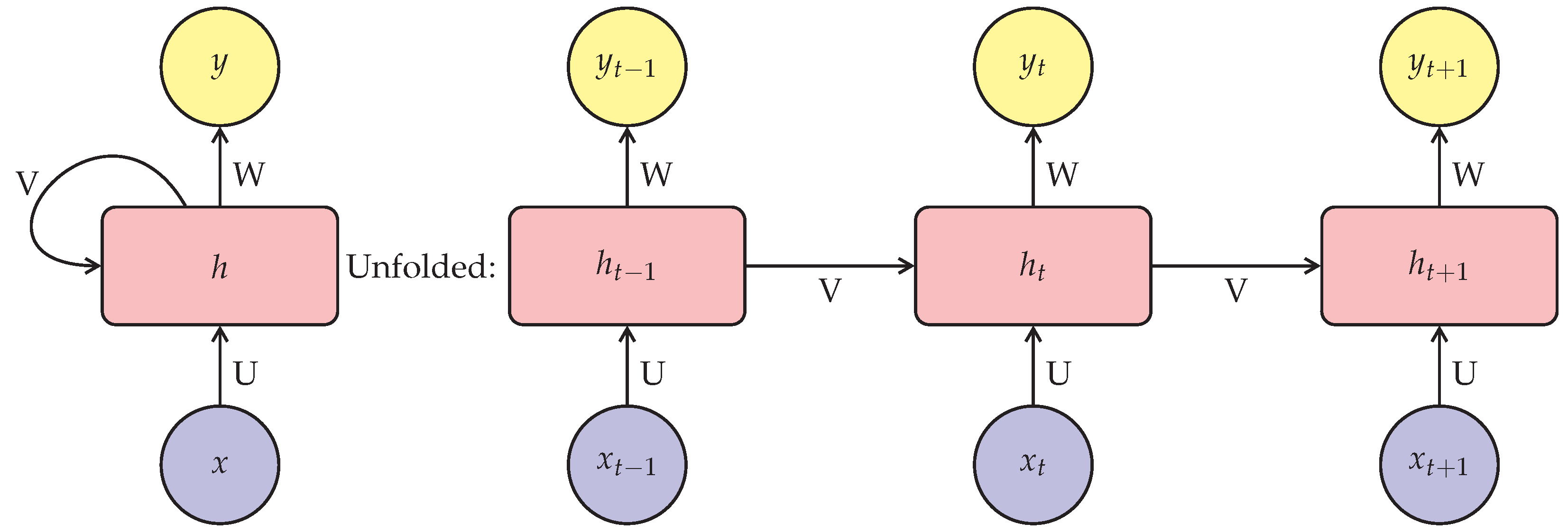
One of the limitations of MLPs is that each sample is processed through the network individually, such that information from previous samples are lost. RNNs were created as a way to provide some memory to a neural network such that they can better perform inference on datasets with sequential dependencies [28]. Depicted in Figure 7 in both a rolled and unrolled fashion, one can see that these networks consider samples at some time t. The input to the RNN at a time t consists of the state of the network from time $t-1$ and the current input $X_t$ [28]. This is visualized in Figure 7 with the specific calculation used in this work provided in Equation (14) [28]

$$h_t=tanh(X_t{U}^T+b+h_{t-1}{V}^T+c)$$

(14)

where $X_t$ is the input at timestep t; U and b are the weights and bias associated with the input; $h_{t-1}$ is the hidden state of the previous time step with V and c being the respective weights and bias for the previous hidden state. The output can then be calculated using Equation (15) [26]:

$$y_t=h_t{W}^T+d$$

(15)

where $h_t$ is defined by Equation (14), with W and d being the weights and bias associated with the output.

Similar to MLPs, RNNs utilize a loss function and a gradient descent based backpropagation optimization, backpropagation through time (BPTT), to perform learning of the network parameters. There are several variants to RNNs, such that they can provide an output at each time step or a single output after a sequence has been processed, as used in this work.

2.5. Long Short-Term Memory Networks

Long short-term memory (LSTM) networks were created to overcome issues encountered when training RNNs such as vanishing and exploding gradients [29]. In addition, they have shown the ability to successfully perform inference on tasks that require long-lasting memory [26]. The main differences between the RNN depicted in Figure 7 and LSTMs include cells with self-loops and a series of gates that control the flow of memory through the network [29]. These gates, which are controlled by learned parameters of the network, include the input gate, forget gate, and output gate. For each cell, the input gate controls whether a given feature will be accumulated within the cell. The state unit of a cell contains the self-loop, which is controlled by the forget gate. The output gate determines a given cell’s output. Each of these gates are generally neurons with learned parameters and a sigmoid activation function. The relevant LSTM calculations are shown in Equations (16)–(21) [30].

$$\begin{array}{cc}\hfill i_t& =sigmoid(W_{ii}{x}_t+b_{ii}+W_{hi}{h}_{t-1}+b_{hi})\hfill \end{array}$$

(16)

$$\begin{array}{cc}\hfill f_t& =sigmoid(W_{if}{x}_t+b_{if}+W_{hf}{h}_{t-1}+b_{hf})\hfill \end{array}$$

(17)

$$\begin{array}{cc}\hfill g_t& =tanh(W_{ig}{x}_t+b_{ig}+W_{hg}{h}_{t-1}+b_{hg})\hfill \end{array}$$

(18)

$$\begin{array}{cc}\hfill o_t& =sigmoid(W_{io}{x}_t+b_{io}+W_{ho}{h}_{t-1}+b_{ho})\hfill \end{array}$$

(19)

$$\begin{array}{cc}\hfill c_t& =f_t\odot c_{t-1}+i_t\odot g_t\hfill \end{array}$$

(20)

$$\begin{array}{cc}\hfill h_t& =o_t\odot tanh\left(c_t\right)\hfill \end{array}$$

(21)

In these equations, $i_t$, $f_t$, $o_t$ are the input, forget, and output gates, respectively; $g_t$ is the cell activation; $c_t$ is the cell state at time t; $h_t$ is the hidden state at time t; $h_{t-1}$ is the hidden state of the previous time step; and $c_{t-1}$ is the cell state at the previous time step. Additionally, ⊙ is the Hadamard product, with W and b representing the various weight and bias vectors of the network. It should be noted that we do not use the LSTM calculations that make use of projections as outlined in the proposed LSTM architecture of [30]. While this makes the LSTM simpler in structure, it does not impact our main goal of comparing its performance between different sets of input features.

2.6. Performance Metrics

In this section, we define the key metrics used to evaluate the performance of using autoencoder feature residuals as input to downstream classifiers. As we are generally assessing comparative performance between X and autoencoder feature residuals, we make use of the mean f1-score from multiple experiment executions.

2.6.1. f1-Score

We use the f1-score as the performance metric to assess how well classifiers are able to distinguish between benign and attack network data. The f1-score, defined in Equation (22), is the harmonic mean of the precision and recall performance metrics [26].

$$\mathrm{f}1-\mathrm{score}=\frac{2\ast precision\ast recall}{precision+recall}$$

(22)

2.6.2. Kolmogorov–Smirnov Test

To add additional statistical measures between our mean f1-scores, we perform a two-sample Kolmogorov–Smirnov test (KS test). The two-sample KS test takes two samples and provides a statistic defined by Equation (23):

$$\mathrm{D}=\underset{u}{sup}|F_m\left(u\right)-G_n\left(u\right)|$$

(23)

where $F_m$ is the empirical distribution function of one sample containing m data points and $G_n$ is the empirical distribution function of a sample containing n data points [31]. We have u as the union of both samples used for comparison, where the statistic returned is the supremum of the absolute value of the differences between the two distributions across u [31]. In our case, we have $F_m$ be the empirical distribution function for results using X as input features and $G_n$ be our method’s results. In this work, $m=n$, as we take ten runs of each experiment for comparison. The KS test statistic is used to determine if the two input samples are from the same distribution [31]. When the associated p-values for this statistic are less than or equal to 0.05, we can reject the null hypothesis that the two samples come from the same distribution. In Section 3, we include these p-values along with our final reported performance measures when comparing our methodology to only using X as input to a classifier.

2.7. General Experiment Set Up

We used a common experiment setup throughout our work while varying the dataset, feature set, and classifier used for the given experiment. This process is depicted in Figure 1, where we initially train an autoencoder using only benign network flow data for 500 epochs. The following steps use this trained autoencoder to produce one of the feature sets depicted in Figure 8 and then train a downstream classifer. All experiments were executed ten times using up to 500,000 samples.

2.8. Model Details

We used the same general autoencoder and classifier structures across all datasets and data encodings that were explored. We found it necessary to change the number of nodes in each layer of the models to account for differences in each data encoding. It was noticed that in general, the autoencoder reconstruction loss was higher when accounting for the sparse encoding, which has only 35 features. We believe this is due to differences in the data encodings, as explained in Section 2.9, as opposed to the adjustments made to the autoencoder structure.

2.8.1. Autoencoder Model

The autoencoder model was determined using previous studies [7], which had the goal of performing well across a broad range of network intrusion datasets as opposed to being optimized for each dataset. With a bottleneck layer size of 12, and 6 layers used to construct the encoder and decoder, we found that the ReLU activation function worked well. We note that no activation function was used for the final output layer. Additionally, we trained using the Adadelta optimizer set with a learning rate of 1.0 to minimize the loss based on the mean-squared error (MSE) loss function. In addition, we utilized a batch size of 128 for training the autoencoders, as with smaller batch sizes, training would experience collapsing gradients on certain datasets.

Table 1. Table from [6]. The details of the two main autoencoder structures used in our research. We note only slight variations in the number of nodes per layer to account for data encoding differences, while keeping the size of the bottleneck layer 12 for both structures. The autoencoders use the Adadelta optimization function with a learning rate of 1.0 and mean squared error for the loss function.

	NFV2 AE	Sparse Encoding AE
Input Dimension	39	35
Encoder Layer 1	34	31
lActivation	ReLU	ReLU
Encoder Layer 2	29	27
Activation	ReLU	ReLU
Encoder Layer 3	24	23
Activation	ReLU	ReLU
Encoder Layer 4	19	19
Activation	ReLU	ReLU
Encoder Layer 5	14	15
Activation	ReLU	ReLU
Encoder Layer 6	12	12
Activation	ReLU	ReLU
Decoder Layer 1	14	15
Activation	ReLU	ReLU
Decoder Layer 2	19	19
Activation	ReLU	ReLU
Decoder Layer 3	24	23
Activation	ReLU	ReLU
Decoder Layer 4	29	27
Activation	ReLU	ReLU
Decoder Layer 5	34	31
Activation	ReLU	ReLU
Decoder Layer 6	39	35

shows the details of the autoencoders used.

2.8.2. Multilayer Perceptron Model

We based our MLP classifier on the work presented in [32], which provides a performance baseline across the datasets explored. We use four layers in the MLP, such that each hidden layer contains 10 output nodes, with the final layer providing a single output. The ReLU activation function was used for each layer except for the final layer, where a sigmoid function was applied. Binary cross entropy was used for the loss function, along with the Adam optimizer configured with a learning rate of 0.001.

Table 2. Table from [6]. The details of the MLP classifiers used in our research. We note only slight variations in the number of nodes in the input layer to account for data-encoding differences, while keeping the size of the remaining layers constant at 10 (aside from the final output). The classifiers use the Adam optimization function with a learning rate of 0.001 and binary cross entropy for the loss function.

	Input Dimension	Output Dimension	Activation
Input Layer	Multiple of 39 or 35	10	ReLU
Layer 1	10	10	ReLU
Layer 2	10	10	ReLU
Layer 3	10	1	Sigmoid

shows the details of the MLP classifiers.

2.8.3. Recurrent Models

Both the RNN and LSTM models used in this work were unidirectional. The model architecture for our recurrent models was found through ablation studies that assessed appropriate sequence lengths, recurrent layers, and hidden state sizes to use. For this work, we used a constant sequence length of 25, two recurrent layers with a hidden state size of 24, and a final fully connected layer. Each recurrent layer used the tanh activation function, and a final sigmoid activation was performed on the output of the fully connected layer. We used the default initialization strategy provided by PyTorch (https://pytorch.org/, accessed on 12 June 2023) for the initialization of hidden and cell states in our recurrent models. Binary cross entropy was used for the loss function, along with the Adam optimizer configured with a learning rate of 0.001. The loss was based on the classifier performance predicting the final netflow sample in a given sequence as being attack or benign. The details of the recurrent models are provided in

Table 3. Architecture of the RNN classifiers used. The input layer takes in a multiple of 35 features, as these models use the sparse encoding of our datasets. The two recurrent layers each have a hidden state size of 24, with the final fully connected layer providing the final output. We use tanh for all recurrent layers and apply a sigmoid activation function to the final fully connected layer. The Adam optimizer with a learning rate of 0.001 is used along with the binary cross entropy loss function. Note that this architecture was used for both the RNN and LSTM models used for classification.

	Input Dimension	Hidden Dimension	Output Dimension	Activation
RNN/LSTM Layer 1	Multiple of 35	24	24	tanh
RNN/LSTM Layer 2	24	24	24	tanh
Fully Connected Layer	24	-	1	Sigmoid

.

2.9. Datasets

Here, we provide an overview of the datasets chosen to evaluate the performance of autoencoder feature residuals. The datasets used are publicly available benchmark datasets that are commonly used for the assessment of NID techniques. In particular, we utilize benchmark datasets with up-to-date attacks and which cover various network environments such as a university network as well as several Internet of Things (IoT) settings. By choosing multiple NID datasets, we are able to assess how well our technique is able to generalize across different network architectures.

2.9.1. Netflow V2 Datasets

To evaluate the performance of autoencoder feature residuals in conjunction with a MLP, we used the four datasets produced in [33], which we refer to collectively as NFV2. These datasets were built using well-known public datasets, are easily accessible, and all use a standard feature set based on NetFlow v9 [34]. The researchers of [33] took the source packet captures from UNSW-NB15 [35], BoT-IoT [36], ToN-IoT [37], and CSE-CIC-IDS2018 [38] and transformed them into a set of 43 features, making comparisons across the datasets efficient. We refer the reader to [33] for specific details regarding these datasets.

2.9.2. Sparse Encoding Derived from Nfv2 Datasets

In addition, we took the NFV2 datasets and restructured their features using the method outlined in previous work [7] to compare our performance across different encodings of the same data. The notable differences between this encoding compared to NFV2 are that it is dominated by one-hot encodings and contains fewer statistical features. The numerical features that are included are based on those we can calculate using byte and packet counts. The details of this encoding are provided in

Table 4. Table from [6]. The features of the sparse data encoding derived from NFV2.

Feature (Type)	Description
communication_type (OHE)	L4_[SRC|DST]_PORT
protocol (OHE)	PROTOCOL
destination_bytes_per_second (Float)	Natural log
destination_packets (Float)	Natural log
destination_packets_per_second (Float)	Natural log
duration (Float)	Duration in seconds
packets_per_second (Float)	Natural log
source_bytes_per_second (Float)	Natural log
source_packets (Float)	Natural log
source_packets_per_second (Float)	Natural log
total_bytes (Float)	Natural log
total_bytes_per_second (Float)	Natural log
total_destination_bytes (Float)	Natural log
total_packets (Float)	Natural log
total_source_bytes (Float)	Natural log
label (Binary)	1 = attack

. We found that the consolidation of multiple protocol values into a single feature of our one-hot encodings resulted in the generation of additional duplicate rows compared to the original dataset. Based on this finding, we dropped duplicates in the dataset only after the final encoding of features was complete, to ensure no contamination of our validation and test data splits.

2.9.3. Datasets Used with Recurrent Classifiers

Due to the fact that the NFV2 datasets do not contain the start time of each flow, we are unable to use it for analyzing the performance of autoencoder feature residuals with recurrent methods. For this reason, we performed our sparse encoding described in Section 2.9.2 on the originally provided netflow data in the UNSW-NB15 [39], ToN-IoT [37], and CTU-13 [40] datasets. The CTU-13 dataset focuses on 13 botnet scenarios, from which we focus our analysis on scenarios 6, 9, and 13. These scenarios were chosen for their suitability to find appropriate training, validation, and test splits that account for the temporal nature of recurrent methods. In general, these scenarios have sufficiently continuous periods of attack throughout their duration, such that we could easily sample sequences of data suitable to use for training and assessing the performance of supervised recurrent models.

2.9.4. General Data Preprocessing Steps

The general preprocessing steps performed on all datasets consisted of the following operations:

• Removing all IP address and port features from the original dataset;
• Dropping rows containing missing values;
• Dropping rows containing invalid negative values;
• Applying min–max normalization on numerical features.

3. Results and Discussion

In this section, we provide the details of our experiments using autoencoder feature residuals and present our empirical results. Incorporated into the presentation of results, we provide a discussion and analysis regarding how these results support the usage of autoencoder feature residuals in place of an original feature set for network intrusion detection.

3.1. Experiments with Feedforward Networks

The preprocessing steps outlined in Section 2.9.4 are augmented with a specialized sampling methodology for our experiments with feedforward networks. For these experiments, we present a single netflow sample to the multilayer perceptron to classify. We found it was sufficient to train the multilayer perceptron classifier for 100 epochs. Stratified random splits of the data consisting of 70/15/15% proportions for training, validation, and testing, respectively, were used to assess performance. Final reported performance measurements are based on the mean results of ten experiments using our holdout test set. We note that dropping the IP address and port features from the NFV2 datasets resulted in additional duplicate rows being present, which we dropped. This caused a slight reduction in our baseline f1-scores (generally a difference of less than 0.1) using the original features of the NFV2 datasets compared to the figures reported in [32].

3.1.1. Substituting X with S

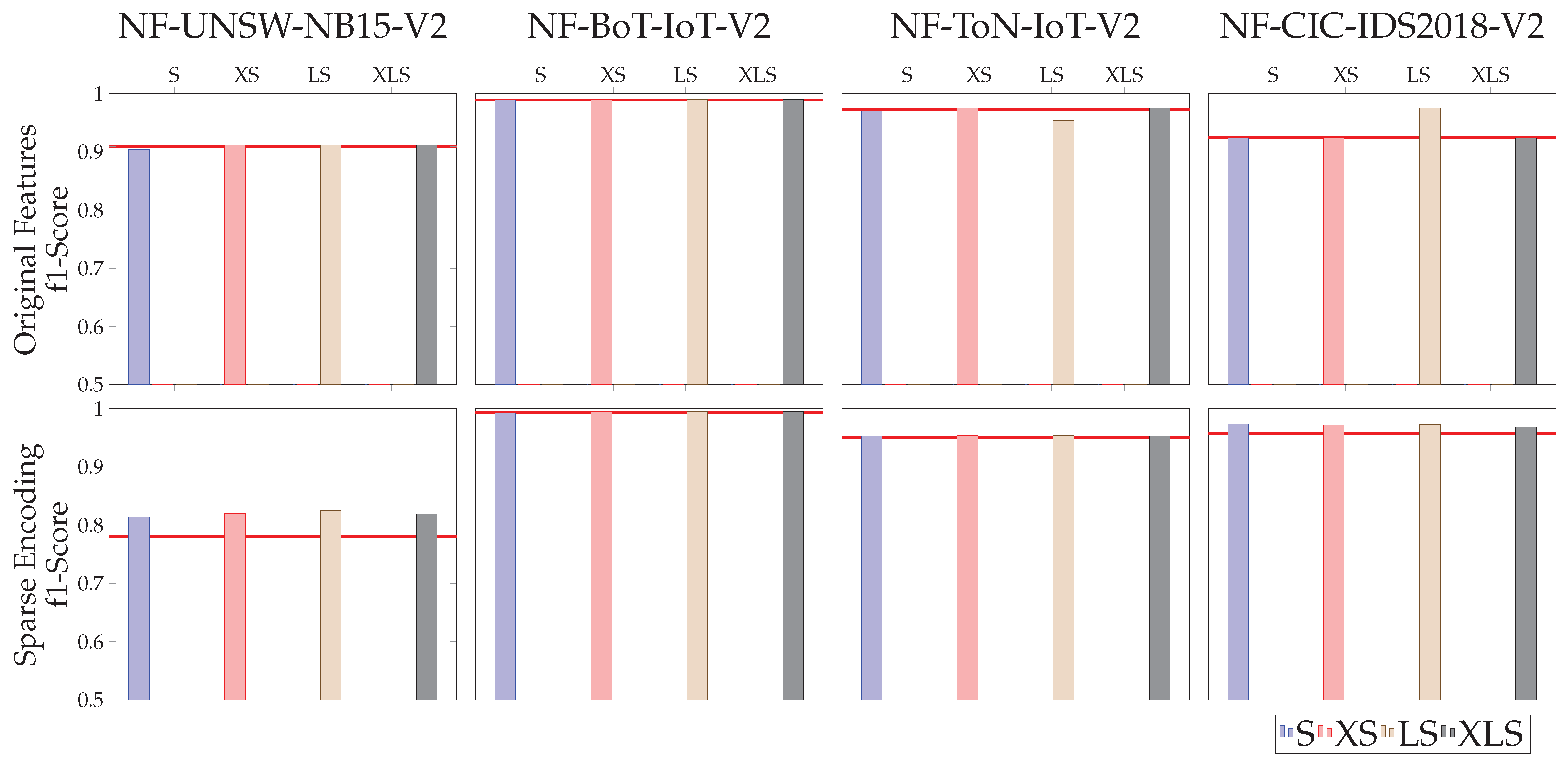
We first assess our performance from the purview of using S as a replacement for X when using an MLP as the classifier. In

Table 5. Table from [6]. Mean f1-score test results based on ten experiment executions using our feature sets. The p-values are derived from the Kolmogoriv–Smirnov test defined in Section 2.6.2. The color coding associates our results with exceeding, meeting, or degrading performance compared to X using green, blue, and orange, respectively. From this table, it can be observed that using S alone or in combinations with X and L generally performs at least as well as using X alone in terms of classification performance, making these combinations of features generally safe to use in place of only using X.

	NF-UNSW-NB15-V2		NF-BoT-IoT-V2		NF-ToN-IoT-V2		NF-CSE-CIC-IDS2018-V2
	f1-Score	p-Value	f1-Score	p-Value	f1-Score	p-Value	f1-Score	p-Value
X	0.909		0.989		0.973		0.924
S	0.904	0.052	0.989	0.418	0.970	0.012	0.924	0.787
XS	0.912	0.052	0.990	0.052	0.975	0.001	0.924	0.168
LS	0.912	0.018	0.990	0.075	0.975	0.011	0.925	0.052
XLS	0.912	0.052	0.990	0.168	0.975	0.003	0.924	0.418

, and visualized in Figure 9, one can observe the mean f1-scores from ten experiment executions for using X and S as input features to a classifier using the NFV2 family of datasets. It is evident that the performance of S as a replacement for X yields comparable results with supporting p-values for the NF-UNSW-NB15-V2, NF-BoT-IoT-V2 and NF-CSE-CIC-IDS2018-V2 datasets. In the cases where a drop in f1-score was observed, we note that it was in magnitudes that would be considered practically irrelevant. One primary example of this is for the NF-ToN-IoT-V2 dataset, where S performed with an f1-score of only 0.003 less than X. To demonstrate how this behavior can arise, one can observe Figure 10, which shows 100 samples of our data. Here, the reconstruction of benign data is done well; however, we would ideally like to see less data in the reconstructions of attack samples. In cases such as this, large autoencoder feature residuals in the benign samples combined with too few in the attack samples can cause a performance reduction. Despite these areas for improvement, our performance remains comparable to using the original feature set.

The overall takeaway from these results is that one could use S as a drop-in replacement for X while maintaining classifier performance. This supports an overall finding that using autoencoder feature residuals, despite strictly removing data from X, is able to retain the most important feature characteristics needed to detect network attacks. In addition, in Section 3.3, we show that using S has additional benefits compared to using X in terms of potential data compression.

3.1.2. Supporting X with S

Additionally at our disposal when using autoencoder feature residuals is forming feature sets using S in combination with X and L. We see in Table 5, and visualized in Figure 9, that combining S with X and L produces results at least as good as using solely X, and in several cases the results are improved. For example, we see statistically significant improvements in performance for many of the combinations that include S on the NF-UNSW-NB15-V2 and NF-ToN-IoT-V2 datasets. We do note that these improvements are likely not substantial enough to deem one feature combination to be preferred over the others from a practical perspective.

3.1.3. Improving Performance on Sparse Datasets

In this set of experiments, we took the data from the NFV2 datasets and encoded it as was carried out in [7] to compare performance across different encodings of the same data. We note that the baseline performance of X here is significantly worse on the UNSW-NB15 dataset compared to the original NFV2 dataset, while the other baseline results are comparable. Notably, Table 6 and the bottom row of Figure 9 show that using S or feature combinations including S provides a substantial increase in f1-score, with this encoding applied to the UNSW-NB15 data. Overall, the results reported show our technique strictly meeting or exceeding the performance of X for this sparse encoding of the NFV2 datasets.

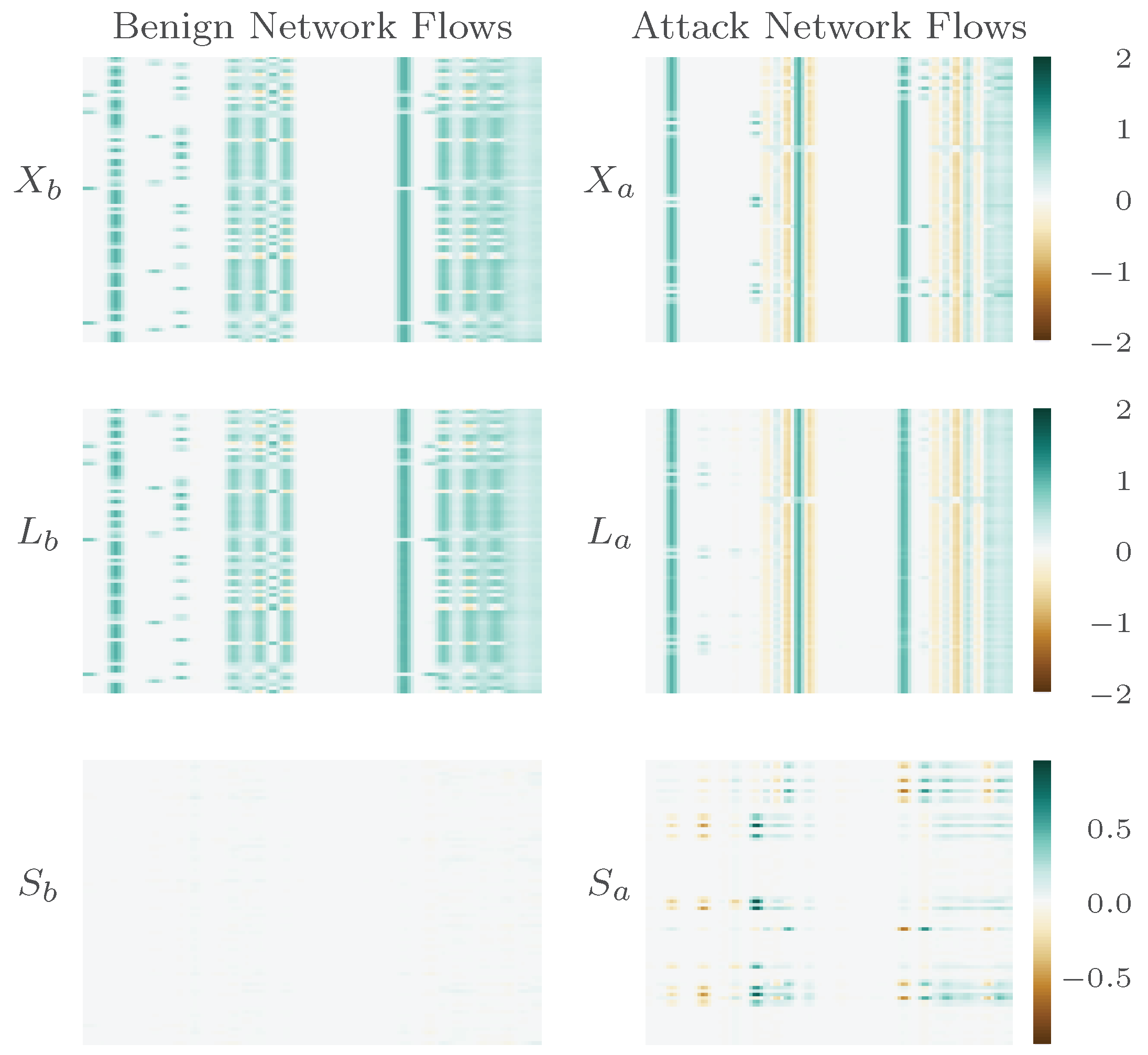
We observe the impact of our technique through a comparison of the original scores for the CSE-CIC-IDS2018-V2 datasets reported in [33] to our much simpler encoding, which contains less insight into network activity. In the original work, an f1-score of 0.97 was obtained using the dense features consisting of 39 Netflow v9 statistics. During our experiments, we obtained a baseline score of only 0.958 when using X, but were able to boost that score to 0.974 when using S. While this only meets the score of the original work, we note that it is doing so by taking an inferior encoding and then making the data more easily accessible to the downstream classifier.

Table 7. A comparison of our mean f1-scores using our feature sets as input to an MLP to the baseline f1-scores for the NFV2 datasets reported in [33]. We see that in general, our feature sets reach comparable performance to the original scores, making the feature sets viable alternatives to using an original set of features.

Dataset	f1-Score from [33]	Our f1-Score	Our Features
NF-UNSW-NB15-V2	0.97	0.91	XS, LS, or XLS
NF-BoT-IoT-V2	1.00	1.00	Sparse encoding; S, XS, LS, or XLS
NF-ToN-IoT-V2	1.00	0.98	XS, LS, or XLS
NF-CSE-CIC-IDS2018-V2	0.97	0.97	Sparse encoding; S, XS, LS, XLS

compares the f1-scores using our feature sets to the originally reported metrics for the NFV2 datasets [33]. In Figure 11, one can observe 100 samples of the sparse encoding applied to the NF-CSE-CIC-IDS2018-V2 test data, where the autoencoder does extremely well at reconstructing benign network flows compared to attack network flows. The sparsity observed in $S_b$ in the bottom left-hand side of the plot compared to the large autoencoder feature residuals in $S_a$ in the bottom right-hand side of the plot both contribute to the improvement seen over using X for classification. While it remains unclear if using autoencoder feature residuals is specifically effective on sparse encodings, this analysis shows that its impact may vary depending on how a dataset is encoded.

Table 6. Table from [6]. Mean f1-score test results based on ten experiment executions using our features sets using an inferior sparse encoding. The p-values are derived from the Kolmogorov–Smirnov test defined in Section 2.6.2. The color coding associates our results with exceeding, meeting, or degrading performance compared to X using green, blue, and orange, respectively. It can be seen that using S and feature combinations including S often outperform using X. In other cases, these combinations generally perform at least as well as just using X.

	NF-UNSW-NB15-V2		NF-BoT-IoT-V2		NF-ToN-IoT-V2		NF-CSE-CIC-IDS2018-V2
	f1-Score	p-Value	f1-Score	p-Value	f1-Score	p-Value	f1-Score	p-Value
X	0.780		0.994		0.950		0.958
S	0.814	0.012	0.993	0.994	0.953	0.168	0.974	0.000
XS	0.820	0.003	0.995	0.787	0.954	0.012	0.972	0.000
LS	0.825	0.000	0.995	0.418	0.954	0.012	0.973	0.000
XLS	0.819	0.000	0.995	0.787	0.953	0.052	0.969	0.000

Table 6. Table from [6]. Mean f1-score test results based on ten experiment executions using our features sets using an inferior sparse encoding. The p-values are derived from the Kolmogorov–Smirnov test defined in Section 2.6.2. The color coding associates our results with exceeding, meeting, or degrading performance compared to X using green, blue, and orange, respectively. It can be seen that using S and feature combinations including S often outperform using X. In other cases, these combinations generally perform at least as well as just using X.

	NF-UNSW-NB15-V2		NF-BoT-IoT-V2		NF-ToN-IoT-V2		NF-CSE-CIC-IDS2018-V2
	f1-Score	p-Value	f1-Score	p-Value	f1-Score	p-Value	f1-Score	p-Value
X	0.780		0.994		0.950		0.958
S	0.814	0.012	0.993	0.994	0.953	0.168	0.974	0.000
XS	0.820	0.003	0.995	0.787	0.954	0.012	0.972	0.000
LS	0.825	0.000	0.995	0.418	0.954	0.012	0.973	0.000
XLS	0.819	0.000	0.995	0.787	0.953	0.052	0.969	0.000

3.2. Experiments with Recurrent Networks

We used a slightly different methodology to preprocess the data used to analyze recurrent classifiers compared to the methodology outlined in Section 3.1. After performing the general data-preprocessing steps outlined in Section 2.9.4, we then took contiguous splits of the datasets such that the training data were strictly prior to the validation data and test data. Similarly, the test data split was strictly after the validation split. This was carried out to ensure that our training data did not contain any information from future periods of the scenario that would be used for assessment of the model. Additionally, splits in proportion to 50/25/25% (training/validation/test) were used in order to avoid introducing optimistic results due to any time bias between the training and test data.

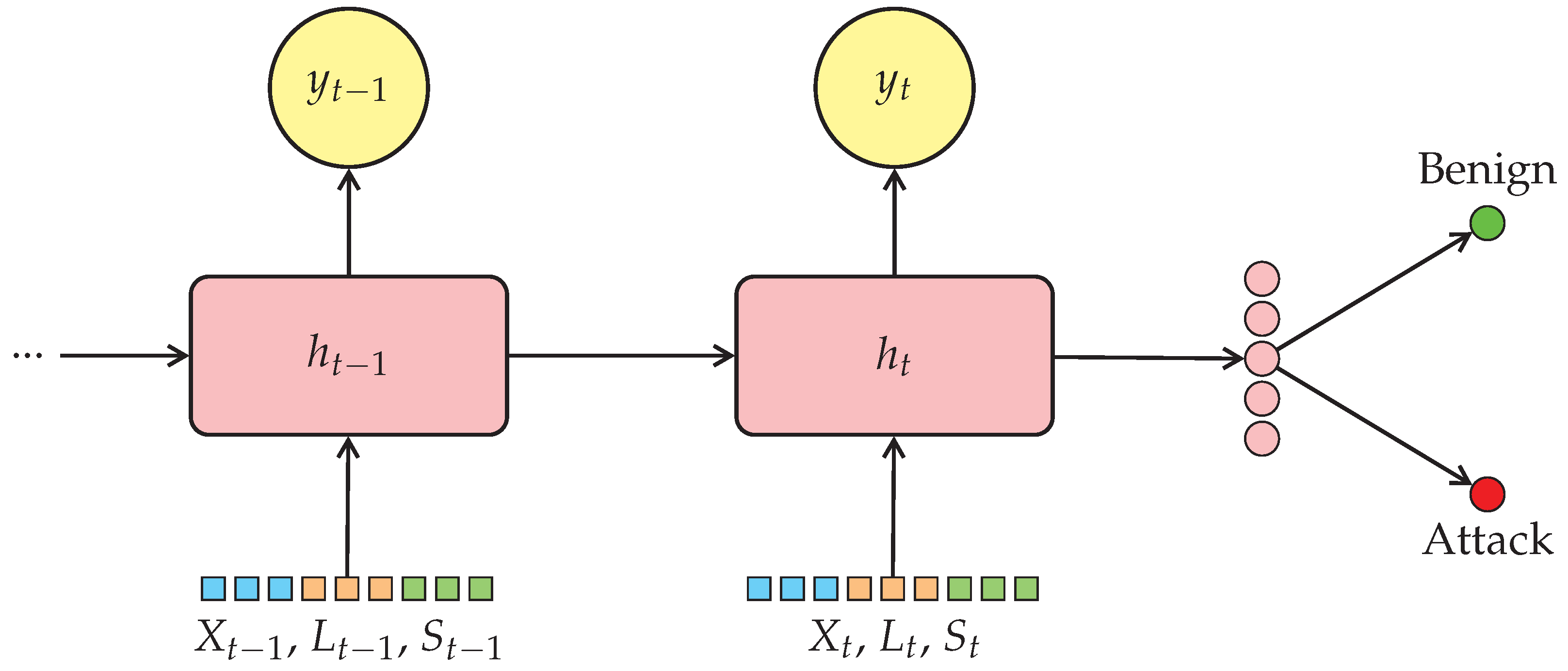
For these experiments, we found it necessary to train each classifier for 500 epochs. A single sample presented to the recurrent neural networks on which we make a classification consists of 25 consecutive netflow samples ordered by flow start time. The features used for each netflow sample consisted of our feature sets created using autoencoder feature residuals. For each input sequence, we predicted if the final sample in the sequence was attack or benign. This can be seen visualized in Figure 12, where we show a portion of a recurrent model taking in a sequence of netflow samples, where each sample is represented by X, L, and S. When using our feature sets as input to RNNs, the calculation of the hidden state is performed using Equation (24):

$$h_t=tanh({\overline{XLS}}_t{U}^T+b+h_{t-1}{V}^T+c)$$

(24)

where the input is now $\overline{XLS}$ to indicate some combination of X, L, and S concatenated together. Similarly, the equations presented in Section 2.5 for an LSTM model are adjusted, as noted in Equations (25)–(30).

$$\begin{array}{cc}\hfill i_t& =sigmoid(W_{ii}{\overline{XLS}}_t+b_{ii}+W_{hi}{h}_{t-1}+b_{hi})\hfill \end{array}$$

(25)

$$\begin{array}{cc}\hfill f_t& =sigmoid(W_{if}{\overline{XLS}}_t+b_{if}+W_{hf}{h}_{t-1}+b_{hf})\hfill \end{array}$$

(26)

$$\begin{array}{cc}\hfill g_t& =tanh(W_{ig}{\overline{XLS}}_t+b_{ig}+W_{hg}{h}_{t-1}+b_{hg})\hfill \end{array}$$

(27)

$$\begin{array}{cc}\hfill o_t& =sigmoid(W_{io}{\overline{XLS}}_t+b_{io}+W_{ho}{h}_{t-1}+b_{ho})\hfill \end{array}$$

(28)

$$\begin{array}{cc}\hfill c_t& =f_t\odot c_{t-1}+i_t\odot g_t\hfill \end{array}$$

(29)

$$\begin{array}{cc}\hfill h_t& =o_t\odot tanh\left(c_t\right)\hfill \end{array}$$

(30)

Final reported performance measurements are based on the mean results of ten experiments using our holdout test set.

Results Using Recurrent Classifiers

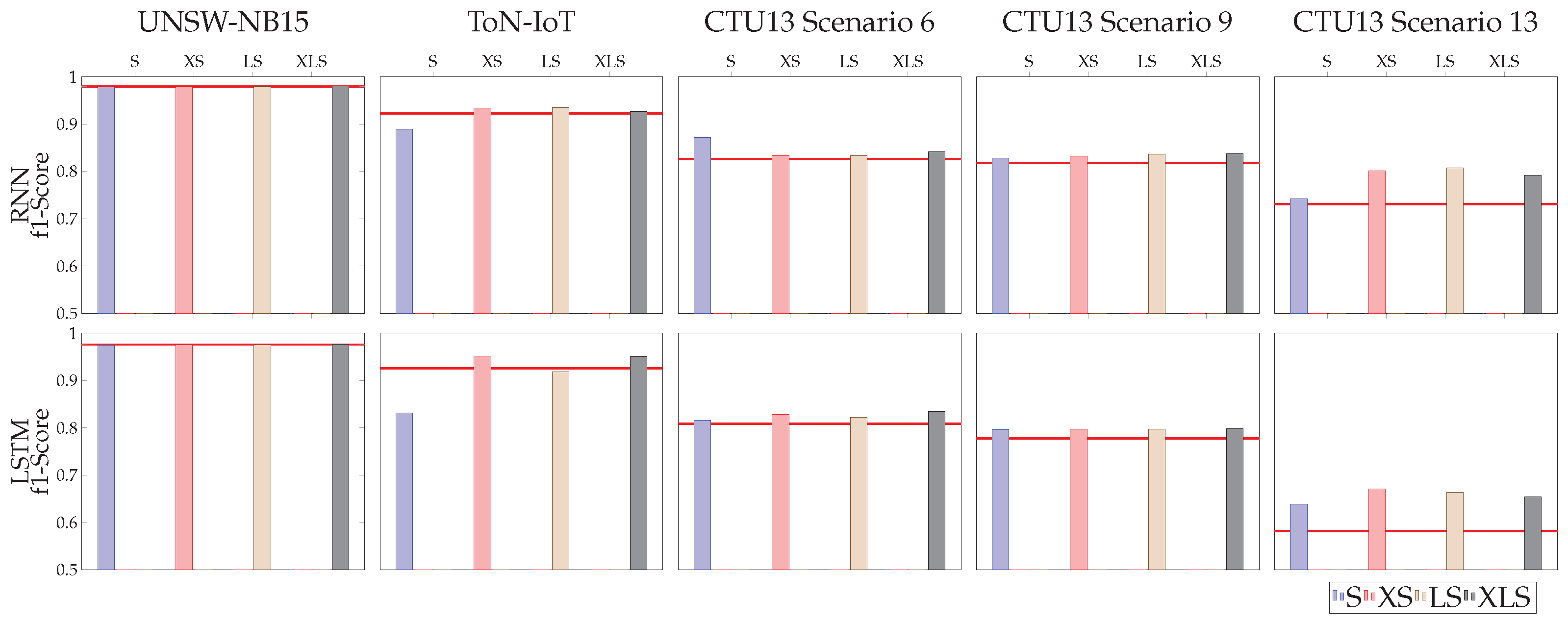
When using recurrent architectures for our classifier, one can see from

Table 8. Mean f1-score test results based on ten experiment executions using S in combination with X and L as input to an RNN classifier using the alternative sparse encoding. p-values using the Kolmogorov–Smirnov test are provided, where values greater than 0.05 indicate the f1-scores were likely drawn from the same distribution. Values in blue indicate an f1-score and p-value that support comparable performance compared to X. Values in green indicate an f1-score and p-value that support improved performance compared to X. Values in orange indicate an f1-score and p-value that support degraded performance compared to X.

	UNSW-NB15		ToN-IoT		CTU13 Scenario 6		CTU13 Scenario 9		CTU13 Scenario 13
	f1-Score	p-Value	f1-Score	p-Value	f1-Score	p-Value	f1-Score	p-Value	f1-Score	p-Value
X	0.980		0.923		0.826		0.818		0.731
S	0.979	0.168	0.889	0.012	0.872	0.000	0.828	0.168	0.742	0.418
XS	0.980	0.994	0.934	0.168	0.834	0.168	0.833	0.002	0.801	0.002
LS	0.980	0.787	0.935	0.002	0.834	0.052	0.837	0.000	0.808	0.002
XLS	0.981	0.052	0.927	0.012	0.842	0.052	0.838	0.000	0.792	0.012

and

Table 9. Mean f1-score test results based on ten experiment executions using S in combination with X and L as input to an LSTM classifier using the alternative sparse encoding. p-values using the Kolmogorov–Smirnov test are provided, where values greater than 0.05 indicate the f1-scores were likely drawn from the same distribution. Values in blue indicate an f1-score and p-value that support comparable performance compared to X. Values in green indicate an f1-score and p-value that support improved performance compared to X. Values in orange indicate an f1-score and p-value that support degraded performance compared to X.

	UNSW-NB15		ToN-IoT		CTU13 Scenario 6		CTU13 Scenario 9		CTU13 Scenario 13
	f1-Score	p-Value	f1-Score	p-Value	f1-Score	p-Value	f1-Score	p-Value	f1-Score	p-Value
X	0.976		0.926		0.809		0.778		0.582
S	0.975	0.052	0.832	0.000	0.816	0.168	0.796	0.002	0.639	0.012
XS	0.976	0.418	0.952	0.012	0.828	0.168	0.797	0.000	0.671	0.002
LS	0.976	0.787	0.919	0.012	0.822	0.418	0.797	0.000	0.664	0.002
XLS	0.977	0.052	0.951	0.002	0.835	0.012	0.798	0.000	0.654	0.012

, and visualized in Figure 13, that we achieve similar behavior as reported for feedforward networks when using autoencoder feature residuals as input. In general, using either S on its own, or in combination with other features, we are able to maintain or improve classification performance. While many of these gains are modest, we note several practical improvements in f1-score compared to using X, such as using $XS$ as input to an LSTM classifier on CTU-13 Scenario 13. In this case, the base f1-score of 0.582 was improved to 0.671. We note a drop in performance on the ToN-IoT dataset when using feature sets that include S without the support of X. However, when S was paired with X in a feature set, our technique achieved a significant performance improvement compared to only using X on that same dataset. Additionally, we see performance improvements using autoencoder feature residuals as input to both RNN and LSTM architectures across all the CTU-13 dataset scenarios, demonstrating that this technique may be well-equipped for the detection of botnet attacks.

We note two common conditions encountered when training recurrent models for network intrusion detection. First, it is common to experience some amount of overfitting to training data when working with recurrent models on datasets with a high class imbalance. Additionally, as one moves further out in time for a network intrusion detection scenario, it becomes more likely that the data characteristics change compared to training data [41,42]. As we were focusing these experiments on obtaining a general idea for the performance of autoencoder feature residuals on recurrent networks, we put forth little effort to mitigate these two factors. We note this to show that the general model performance improvements reported in Table 8 and Table 9 over using X demonstrates that using autoencoder feature residuals provides some benefit in mitigating these factors, while requiring little model tuning compared to other methods.

While the focus of this work is on using S, we do recognize that one could also use L or $XL$ as feature combinations in place of X. We found that in general, $XL$ performed comparable to X; however, L generally performed worse than X when using an MLP, RNN, or LSTM classifier. We believe this is in line with our previously reported findings [7], in that the usage of L, or combinations with L, tend to hold some volatility in results dependent on the differences in benign training samples compared to the test data used.

3.3. Data Compression Benefits of S

As noted throughout our results discussion, our technique often only performs as well as X when using S in its place. In these situations, one would want to seek alternative advantages to using S that are not strictly related to classifier performance. One such case that can be considered is the use of S as a way to compress the amount of data that needs to be collected from network resources. Below, we list several assumptions used for consideration of this scenario:

• Both S and X require the same amount of base storage;
• Values in S that are zero are uninteresting because they were perfectly reconstructed;
• There are equal amounts of metadata to indicate what was collected for both X and S.

Taking 500 benign samples of X and S, we report the mean compression ratios in

Table 10. Table from [6]. The compression ratios found using 500 samples of benign data from our datasets. This analysis used the assumptions outlined in Section 3.3. After applying a threshold on values close to zero in S, a higher compression ratio was observed compared to attempts to compress X under the same set of assumptions. In parentheses, we show the mean f1-scores from these experiments, which were comparable to those reported in Table 5 for S.

	NF-UNSW-NB15-V2	NF-BoT-IoT-V2	NF-ToN-IoT-V2	NF-CSE-CIC-IDS2018-V2
X (No Zeros)	1.857	2.254	2.313	2.326
S (No Zeros)	0.000	0.000	0.000	0.000
Thresholded S (No Zeros)	3.168 (0.903)	2.074 (0.989)	3.331 (0.964)	5.075 (0.924)

. Our initial analysis of compression found that no values in S were strictly zero, resulting in poor compression rates. To mitigate this, we empirically determined that any values greater than −0.001 and less than 0.01 could be considered zero without impact to classification performance, and were treated as such for this analysis.

Looking at the compression ratios of the thresholded S, we see that it generally outperformed the compression possible on X based on our assumptions. A higher compression rate was found for X on the NF-BoT-IoT-V2 dataset compared to that of the thresholded S, which is likely due to suboptimal thresholding options for that particular dataset. The finding of a more robust thresholding technique on S for compression purposes, and the exploration of regularizing the autoencoder to induce feature residuals of zero, is left for future work. While this was a simplistic view of a compression scenario, it shows that S has potential benefits over X beyond classification performance gains that could be explored further in future research.

4. Conclusions

In this work, we explored the application of using autoencoder feature residuals when paired with several architectures of neural networks. Through empirical analysis, it was shown that feature sets using autoencoder feature residuals are suitable drop-in replacements for an original feature set. In general, these feature sets either meet the performance of the original features or, oftentimes, increase classifier performance. We note that our technique strictly removes data from an original feature set, making it an interesting achievement, even when we only match the performance of these features.

In the context of feedforward neural networks, we showed that using feature sets that include autoencoder feature residuals generally increases performance. This was demonstrated using four datasets consisting of various cybersecurity scenarios and across two separate encodings of the data. We then extended our experiments to account for the sequential aspect of network data by using our feature sets as input to RNN and LSTM classifiers. In these experiments, we showed that autoencoder feature residuals can be used successfully across a number of neural network architectures, and are particularly effective for the detection of botnet attacks.

Rounding out the benefits of autoencoder feature residuals, we showed that using autoencoder feature residuals rather than their corresponding original feature set has the advantage of allowing network data to be compressed, which reduces the amount of resources needed for its collection.

References

1. Kim, J.; Shin, N.; Jo, S.Y.; Kim, S.H. Method of intrusion detection using deep neural network. In Proceedings of the 2017 IEEE International Conference on Big Data and Smart Computing (BigComp), Seoul, Republic of Korea, 13–16 February 2017; IEEE: Piscataway, NJ, USA, 2017; pp. 313–316. [Google Scholar]
2. Yang, Z.; Liu, X.; Li, T.; Wu, D.; Wang, J.; Zhao, Y.; Han, H. A systematic literature review of methods and datasets for anomaly-based network intrusion detection. Comput. Secur. 2022, 116, 102675. [Google Scholar] [CrossRef]
3. Andresini, G.; Appice, A.; Mauro, N.D.; Loglisci, C.; Malerba, D. Exploiting the Auto-Encoder Residual Error for Intrusion Detection. In Proceedings of the 2019 IEEE European Symposium on Security and Privacy Workshops (EuroS & PW), Stockholm, Sweden, 17–19 June 2019; IEEE: Piscataway, NJ, USA, 2019. [Google Scholar] [CrossRef]
4. Long, C.; Xiao, J.; Wei, J.; Zhao, J.; Wan, W.; Du, G. Autoencoder ensembles for network intrusion detection. In Proceedings of the 2022 24th International Conference on Advanced Communication Technology (ICACT), Pyeongchang, Republic of Korea, 13–16 February 2022; IEEE: Piscataway, NJ, USA, 2022. [Google Scholar] [CrossRef]
5. Wang, W.; Jian, S.; Tan, Y.; Wu, Q.; Huang, C. Representation learning-based network intrusion detection system by capturing explicit and implicit feature interactions. Comput. Secur. 2022, 112, 102537. [Google Scholar] [CrossRef]
6. Lewandowski, B.; Paffenroth, R. Autoencoder Feature Residuals for Network Intrusion Detection: Unsupervised Pre-training for Improved Performance. In Proceedings of the 2022 21st IEEE International Conference on Machine Learning and Applications (ICMLA), Nassau, Bahamas, 12–14 December 2022; IEEE: Piscataway, NJ, USA, 2022; pp. 1334–1341. [Google Scholar]
7. Lewandowski, B.; Paffenroth, R.; Campbell, K. Improving Network Intrusion Detection Using Autoencoder Feature Residuals. In Proceedings of the 2022 4th International Conference on Data Intelligence and Security (ICDIS), Shenzhen, China, 24–26 August 2022; IEEE: Piscataway, NJ, USA, 2022; pp. 31–39. [Google Scholar]
8. Mirsky, Y.; Doitshman, T.; Elovici, Y.; Shabtai, A. Kitsune: An ensemble of autoencoders for online network intrusion detection. arXiv 2018, arXiv:1802.09089. [Google Scholar]
9. Bishop, C.M.; Nasrabadi, N.M. Pattern Recognition and Machine Learning; Springer: Berlin/Heidelberg, Germany, 2006; Volume 4. [Google Scholar]
10. Song, Y.; Hyun, S.; Cheong, Y.G. Analysis of Autoencoders for Network Intrusion Detection. Sensors 2021, 21, 4294. [Google Scholar] [CrossRef] [PubMed]
11. Ortega-Fernandez, I.; Sestelo, M.; Burguillo, J.C.; Piñón-Blanco, C. Network intrusion detection system for DDoS attacks in ICS using deep autoencoders. Wirel. Netw. 2023. [Google Scholar] [CrossRef]
12. Zhang, H.; Ge, L.; Zhang, G.; Fan, J.; Li, D.; Xu, C. A two-stage intrusion detection method based on light gradient boosting machine and autoencoder. Math. Biosci. Eng. 2023, 20, 6966–6992. [Google Scholar] [CrossRef]
13. Zhang, T.; Chen, W.; Liu, Y.; Wu, L. An Intrusion Detection Method Based on Stacked Sparse Autoencoder and Improved Gaussian Mixture Model. Comput. Secur. 2023, 128, 103144. [Google Scholar] [CrossRef]
14. Andresini, G.; Appice, A.; Malerba, D. Autoencoder-based deep metric learning for network intrusion detection. Inf. Sci. 2021, 569, 706–727. [Google Scholar] [CrossRef]
15. Habeeb, M.S.; Babu, T.R. Network intrusion detection system: A survey on artificial intelligence-based techniques. Expert Syst. 2022, 39, e13066. [Google Scholar] [CrossRef]
16. Macas, M.; Wu, C.; Fuertes, W. A survey on deep learning for cybersecurity: Progress, challenges, and opportunities. Comput. Netw. 2022, 212, 109032. [Google Scholar] [CrossRef]
17. Fu, Y.; Du, Y.; Cao, Z.; Li, Q.; Xiang, W. A Deep Learning Model for Network Intrusion Detection with Imbalanced Data. Electronics 2022, 11, 898. [Google Scholar] [CrossRef]
18. Nguyen, X.H.; Nguyen, X.D.; Huynh, H.H.; Le, K.H. Realguard: A Lightweight Network Intrusion Detection System for IoT Gateways. Sensors 2022, 22, 432. [Google Scholar] [CrossRef] [PubMed]
19. Yin, Y.; Jang-Jaccard, J.; Xu, W.; Singh, A.; Zhu, J.; Sabrina, F.; Kwak, J. IGRF-RFE: A hybrid feature selection method for MLP-based network intrusion detection on UNSW-NB15 dataset. J. Big Data 2023, 10, 15. [Google Scholar] [CrossRef]
20. Khan, M.A. HCRNNIDS: Hybrid Convolutional Recurrent Neural Network-Based Network Intrusion Detection System. Processes 2021, 9, 834. [Google Scholar] [CrossRef]
21. Ravi, V.; Chaganti, R.; Alazab, M. Recurrent deep learning-based feature fusion ensemble meta-classifier approach for intelligent network intrusion detection system. Comput. Electr. Eng. 2022, 102, 108156. [Google Scholar] [CrossRef]
22. Kherlenchimeg, Z.; Nakaya, N. Network intrusion classifier using autoencoder with recurrent neural network. In Proceedings of the Fourth International Conference on Electronics and Software Science (ICESS2018), Takamatsu, Japan, 5–7 November 2018; pp. 5–7. [Google Scholar]
23. Elsayed, M.S.; Le-Khac, N.A.; Dev, S.; Jurcut, A.D. DDoSNet: A Deep-Learning Model for Detecting Network Attacks. In Proceedings of the 2020 IEEE 21st International Symposium on “A World of Wireless, Mobile and Multimedia Networks” (WoWMoM), Cork, Ireland, 31 August–3 September 2020; pp. 391–396. [Google Scholar] [CrossRef]
24. Han, D.; Wang, Z.; Chen, W.; Zhong, Y.; Wang, S.; Zhang, H.; Yang, J.; Shi, X.; Yin, X. DeepAID: Interpreting and Improving Deep Learning-based Anomaly Detection in Security Applications. In Proceedings of the 2021 ACM SIGSAC Conference on Computer and Communications Security, Virtual, Republic of Korea, 15–19 November 2021. [Google Scholar] [CrossRef]
25. Yehezkel, A.; Elyashiv, E.; Soffer, O. Network Anomaly Detection Using Transfer Learning Based on Auto-Encoders Loss Normalization. In Proceedings of the 14th ACM Workshop on Artificial Intelligence and Security, Virtual Event, Republic of Korea, 15 November 2021; pp. 61–71. [Google Scholar]
26. Goodfellow, I.; Bengio, Y.; Courville, A. Deep Learning; MIT Press: Cambridge, MA, USA, 2016. [Google Scholar]
27. Kramer, M.A. Nonlinear principal component analysis using autoassociative neural networks. AIChE J. 1991, 37, 233–243. [Google Scholar] [CrossRef]
28. Rumelhart, D.E.; Hinton, G.E.; Williams, R.J. Learning Internal Representations by Error Propagation; Technical Report; California University San Diego La Jolla Institute for Cognitive Science: San Diego, CA, USA, 1985. [Google Scholar]
29. Hochreiter, S.; Schmidhuber, J. Long Short-Term Memory. Neural Comput. 1997, 9, 1735–1780. [Google Scholar] [CrossRef] [PubMed]
30. Sak, H.; Senior, A.; Beaufays, F. Long Short-Term Memory Based Recurrent Neural Network Architectures for Large Vocabulary Speech Recognition. arXiv 2014, arXiv:1402.1128. [Google Scholar] [CrossRef]
31. Hodges, J.L. The significance probability of the Smirnov two-sample test. Ark. Mat. 1958, 3, 469–486. [Google Scholar] [CrossRef]
32. Sarhan, M.; Layeghy, S.; Portmann, M. Evaluating Standard Feature Sets Towards Increased Generalisability and Explainability of ML-based Network Intrusion Detection. arXiv 2021, arXiv:2104.07183. [Google Scholar] [CrossRef]
33. Sarhan, M.; Layeghy, S.; Portmann, M. Towards a Standard Feature Set for Network Intrusion Detection System Datasets. Mob. Netw. Appl. 2021, 27, 357–370. [Google Scholar] [CrossRef]
34. Systems, C. Cisco IOS NetFlow Version 9 Flow Record Format. Available online: https://www.cisco.com/en/US/technologies/tk648/tk362/technologies_white_paper09186a00800a3db9.pdf (accessed on 12 June 2023).
35. Moustafa, N.; Turnbull, B.; Choo, K.K.R. An Ensemble Intrusion Detection Technique Based on Proposed Statistical Flow Features for Protecting Network Traffic of Internet of Things. IEEE Internet Things J. 2019, 6, 4815–4830. [Google Scholar] [CrossRef]
36. Koroniotis, N.; Moustafa, N.; Sitnikova, E.; Turnbull, B. Towards the Development of Realistic Botnet Dataset in the Internet of Things for Network Forensic Analytics: Bot-IoT Dataset. arXiv 2018, arXiv:1811.00701. [Google Scholar] [CrossRef] [Green Version]
37. Moustafa, N. A new distributed architecture for evaluating AI-based security systems at the edge: Network TON_IoT datasets. Sustain. Cities Soc. 2021, 72, 102994. [Google Scholar] [CrossRef]
38. Sharafaldin, I.; Lashkari, A.H.; Ghorbani, A.A. Toward generating a new intrusion detection dataset and intrusion traffic characterization. ICISSp 2018, 1, 108–116. [Google Scholar]
39. Moustafa, N.; Slay, J. UNSW-NB15: A comprehensive data set for network intrusion detection systems (UNSW-NB15 network data set). In Proceedings of the 2015 Military Communications and Information Systems Conference (MilCIS), Canberra, ACT, Australia, 10–12 November 2015; pp. 1–6. [Google Scholar] [CrossRef]
40. García, S.; Grill, M.; Stiborek, J.; Zunino, A. An empirical comparison of botnet detection methods. Comput. Secur. 2014, 45, 100–123. [Google Scholar] [CrossRef]
41. Widmer, G.; Kubat, M. Learning in the Presence of Concept Drift and Hidden Contexts. Mach. Learn. 1996, 23, 69–101. [Google Scholar] [CrossRef] [Green Version]
42. Maciá-Fernández, G.; Camacho, J.; Magán-Carrión, R.; García-Teodoro, P.; Therón, R. UGR’16: A new dataset for the evaluation of cyclostationarity-based network IDSs. Comput. Secur. 2018, 73, 411–424. [Google Scholar] [CrossRef] [Green Version]
Figure 1. Figure from [6]. An overview of the process used to generate and perform classification with autoencoder feature residuals. Taking only benign network flow samples, an autoencoder is trained. This trained autoencoder can then be provided with benign and attack network samples to construct a number of novel feature sets using autoencoder feature residuals. These feature sets then train a neural network such that it can effectively classify a given network sample as attack or benign. With both trained models in hand, we can then perform inference on novel samples.
Make 05 00046 g001
Figure 2. In this synthetic motivating example, we show the disadvantages that can arise when using aggregate loss metrics for detecting anomalies. On the left-hand side, we show the autoencoder feature residuals for a benign network flow sample, while the right-hand side shows the autoencoder feature residuals for an attack. The error for both samples is equal; however, it is distributed differently among the features. An aggregate metric such as mean-squared error would calculate the anomaly score the same for both samples, resulting in the benign sample being flagged as a false-positive. Providing the autoencoder feature residuals to a downstream classifier provides the classifier with the opportunity to differentiate the two samples.
Make 05 00046 g002
Figure 3. Sample architecture of the main components of an autoencoder. Depicted in blue are the input features and their respective reconstructions. Depicted in pink are hidden nodes. Depicted in red is the bottleneck layer.
Make 05 00046 g003
Figure 4. Figure from [6]. Here we visualize our notation by showing a benign and attack sample consisting of five features. Representing the value of each feature with color bars, one can see that S b is expected to be sparse and contain less data than S a . Along with this property, L b would contain more data than L a .
Make 05 00046 g004
Figure 5. Figure from [6]. Depicted in this figure is a visualization of the conditions that lead to optimal features to provide to downstream classifiers. Notably, L b = X b , S b = 0 , L a = 0 , and S a = X a , leading to the ability to use either L or S as optimal features for binary classification of network samples.
Make 05 00046 g005
Figure 6. Sample architecture of the main components of a multilayer perceptron. Depicted in blue are the input features. Depicted in pink are nodes of a hidden layer. This network has a single output y 1 , denoted in yellow.
Make 05 00046 g006
Figure 7. Sample architecture of the main components of a recurrent neural network. Depicted in blue are the input features. Depicted in pink are recurrent hidden nodes. The network’s output from each hidden node is denoted as y in yellow.
Make 05 00046 g007
Figure 8. Figure from [6]. The feature sets generated using an autoencoder trained on only benign network flow data in our experiments. X, depicted in cyan, contains five features and represents the original input features. L, depicted in orange, contains five features and represents the autoencoder reconstruction. S, depicted in green, contains five features and represents the autoencoder feature residuals. Each of our experiments uses one of these feature sets to train a downstream classifier.
Make 05 00046 g008
Figure 9. A visualization of our results for using autoencoder feature residuals in conjunction with MLP classifiers in terms of mean f1-scores. The top row visualizes the results from Table 5 and the bottom row visualizes the results from Table 6. The red line in each plot represents the baseline values of X for each dataset. From these plots, one can see that using feature sets that include autoencoder feature residuals meets or exceeds the baseline performance of X.
Make 05 00046 g009
Figure 10. Figure from [6]. One hundred samples from the NF-CSE-CIC-IDS2018-V2 dataset broken out into X, L, and S. Our corresponding classification performance for this dataset showed that S and X performed comparably. We see positive qualities in this data, such as the observation that the autoencoder struggles more to reconstruct network attacks. On the other hand, there remain several prominent autoencoder feature residuals visible in S b in the bottom left-hand side of the plot. These autoencoder feature residuals in S b have the potential to degrade the performance of using S in place of X for classification, leaving room for improvement such that S has the potential to exceed the performance of X.
Make 05 00046 g010
Figure 11. Figure from [6]. One hundred samples from the NF-CSE-CIC-IDS2018-V2 dataset using the inferior sparse encoding broken out into X, L, and S. Our corresponding classification performance for this dataset showed that S improved the performance compared to X. This improvement allowed using an inferior encoding of the data to meet the original performance marks noted on the original dataset from [33]. We note the positive qualities of the data, such as seeing that S b , on the bottom left side of the plot, is sparse, with significantly fewer autoencoder feature residuals than S a .
Make 05 00046 g011
Figure 12. Here, we show the general structure for how the features generated using our technique are used with recurrent models. After samples are processed through our autoencoder to create X, L, and S, combinations of these feature sets are used to represent a single network flow. In this example, we represent a network flow using all three feature sets, referred to as X L S . A sequence of these samples are provided to the recurrent model. The hidden state of the final unit in the recurrent layers is then provided to a fully connected layer, which produces our final prediction of the sequence being an attack or benign sequence. In our experiments, we consider a sequence of network flows to be an attack or benign sequence based on the label of the final netflow sample in the sequence.
Make 05 00046 g012
Figure 13. A visualization of our results for using autoencoder feature residuals in conjunction with recurrent classifiers in terms of mean f1-scores. The top row visualizes the results from Table 8 using an RNN and the bottom row visualizes the results from Table 9 using an LSTM. The red line in each plot represents the baseline values of X for each dataset. From these plots, one can see that using feature sets that include autoencoder feature residuals meets or exceeds using the original features.
Make 05 00046 g013