Biologically Inspired Self-Organizing Computational Model to Mimic Infant Learning

Abstract

Recent technological advancements have fostered human–robot coexistence in work and residential environments. The assistive robot must exhibit humane behavior and consistent care to become an integral part of the human habitat. Furthermore, the robot requires an adaptive unsupervised learning model to explore unfamiliar conditions and collaborate seamlessly. This paper introduces variants of the growing hierarchical self-organizing map (GHSOM)-based computational models for assistive robots, which constructs knowledge from unsupervised exploration-based learning. Traditional self-organizing map (SOM) algorithms have shortcomings, including finite neuron structure, user-defined parameters, and non-hierarchical adaptive architecture. The proposed models overcome these limitations and dynamically grow to form problem-dependent hierarchical feature clusters, thereby allowing associative learning and symbol grounding. Infants can learn from their surroundings through exploration and experience, developing new neuronal connections as they learn. They can also apply their prior knowledge to solve unfamiliar problems. With infant-like emergent behavior, the presented models can operate on different problems without modifications, producing new patterns not present in the input vectors and allowing interactive result visualization. The proposed models are applied to the color, handwritten digits clustering, finger identification, and image classification problems to evaluate their adaptiveness and infant-like knowledge building. The results show that the proposed models are the preferred generalized models for assistive robots.

1. Introduction

The embodiment of an assistive robot in residential areas can support people with their daily routines, provide physical assistance, promote social interactions, and monitor health parameters [1,2]. Taking care of the elderly and autistic children is a massive undertaking and causes tremendous mental stress for caregivers in the long term [3]. Caregivers are also hugely influenced by burnout syndrome. Burnout is an alarming issue impacting teachers’ physical and mental health, leading to emotional exhaustion [4]. The adaption of assistive robots plays a pivotal role in elder care/children care, repetitive task assistance, interactive teaching, and user-dependent services in residential areas, positively impacting individuals [5,6]. Assistive robots require an intelligent human-like decision-making system to tackle real-world problems. The assistive robot mandates the collective functioning of a combination of sensors and actuators to fulfill the necessities of human users. The synergic integration of sensors facilitates the introduction of distinct features at the robot’s disposal. The assistive robot requires an adaptive architecture to combine all of the submodules to process the raw data and produce meaningful decisions. The submodules in the architecture consist of the visual cortex, auditory, and navigation system [7,8,9]. Each module in the architecture utilizes distinct computational models to synergize different sensory input data from various sensors to generate a proper response. The real-time visual cortex submodule analogous to the human visual cortex handles person identification, face identification/recognition, and object/emotion recognition [10,11,12]. The auditory system is elemental for living creatures to acquire information about their surroundings from the sound. The artificial counterpart of the human auditory system is required for assistive robots to provide appropriate assistance and communicate with humans successfully [13]. End-to-end speech recognition models can surpass and replace the traditional hybrid models in assistive robots [14]. Collision avoidance and autonomous navigation with simultaneous localization and mapping (SLAM) are crucial for assistive robots to function in the user environment. The primary task of the navigation system is to determine its current location and estimate the optimal path for the given target position in the working environment. Intensity-SLAM and Edge-SLAM models outperform the existing navigation models in assistive robots [15,16]. The computation models mentioned above are used in assistive robots’ visual, auditory, and navigation modules to tackle the challenges they encounter in their working environment without compromise. However, the key features lacking in assistive robots are associative learning and knowledge rebuilding [17,18]. Furthermore, replacing the distinct computational models with a universal adaptive model benefits assistive robots in explorative learning in unknown territory. The development of artificial cognition for assistive robots is essential as they work with humans, and their primary task is to recognize and understand the presented information for preferable outcomes. Since robots often find it challenging to perform well in unfamiliar and dynamic conditions, they should imitate infant learning to acquire and reform their experience.

1.1. Infant Learning

Infants are good at grasping new skills and gathering knowledge about their surroundings. Adult learning, on the other hand, involves complex cognitive techniques such as reasoning, problem-solving, and decision making. Infant learning models form associations between stimuli and learn to adapt to their environment [19]. These early learning experiences set the stage for future learning and development. To acquire a basic understanding of their surroundings, infants undergo an intense exploration that leads to the continuous organizing and pruning of neuron connections. The formation of new neuronal connections enables infants to interpret sensory information and translate their experience into suitable behavioral responses. Further, the ability to generalize their learning and expertise helps them to solve unfamiliar problems. However, on the functional level, the underlying principles which help in cognition remain an open problem. Several studies attempted to develop novel cognitive architectures for assistive robots to emulate human cognition and learning. ACT-R (short for “Adaptive Control of Thought—Rational”) is a hybrid cognitive architecture that predicts and explains human behaviors such as interaction and cognition [20,21]. Refs. [22,23,24] proposed an integrated cognitive architecture that utilizes distributional reinforcement learning and temporal motivation theory to yield human-like decision making. Studies have shown that human cognition utilizes self-organizing capabilities [25,26]. New behaviors tend to emerge from local and decentralized interactions [27,28]. In the self-organizing model, the order arises from an initially disorganized system by local interactions, and it is capable of regulating and adapting its behavior.

1.2. Need for Self-Organization in Assistive Robots

In an assistive robot, learning starts with acquiring signals in numerous forms from the surroundings. With their learning models, robots need to develop a cognition model without substantial supervision, which needs online training and associative learning. However, the current robot models utilize offline and time-consuming training methods to build new knowledge. Once learned, the robot should undergo retraining to incorporate new world models. Obtaining labeled data is frequently challenging in the human environment, and results suffer from unseen conditions [29]. With unsupervised learning, assistive robots can cluster unlabeled data from patterns, similarities, and differences without prior training, enabling robots to be more practical in human environments. With the elimination of human supervision from the learning process, robots can learn directly from data, allowing explorative learning, thus saving time and effort [30,31,32]. Therefore, for assistive robots, unsupervised exploration-based learning is essential for successful collaboration and operation in daily living environments. It also enhances the ability to learn and generalize human behaviors and gain a shared comprehension of a scenario. Various studies suggest that the human brain employs self-organization to evolve and establish new neuronal connections [25,28,33]. These neuronal connections are created from local environmental interactions [25,26]. Haken [34] proposed that the synergetic connections in the brain use self-organization. The amazingly complex nature of the brain raises the question of how these innumerable cross-connections are connected. Nature adopted self-organization to solve this problem. Human consciousness is a result of sophisticated, dense interconnections. This unique attribute distinguishes humans from animals since it facilitates awareness about self and others. Self-organizing and emergence are fundamental elements of working memory, recurrent learning, and sequential computation in lexicon processing [35]. From the study, [36] advocate that the hierarchical structure, dynamics, and coordination of brain activities are driven by self-organization and emergence. Lloyd [37] shows that the cognitive map in the human brain can be simulated using self-organizing maps.

Employing self-organizing computational models to assistive robots by taking inspiration from nature, enacts new perspectives that result in human-like decision-making capabilities [38,39]. By eliminating humans from the learning process, robots can directly learn from the data available. The features available in the provided data must be identified and clustered for further learning and the decision-making process. In this paper, we propose unsupervised hierarchical computational models for assistive robots. The inclusion of the proposed computational models, in turn, helps assistive robots learn from unfamiliar data from their working environments.

1.3. SOM Models for Assistive Robots

A self-organizing map (SOM) is an unsupervised artificial neural network (ANN) [40]. Traditionally, artificial neural networks apply error correction with backpropagation for their training. Backpropagation frequently uses gradient descent for error corrections. Unlike ANN, SOM employs competitive learning for its training. The algorithm of the SOM follows the biological functioning of neurons. The SOM models can perform well on problems without prior knowledge about the input vectors. This feature allows the model to train on raw, unlabeled data. Essentially, the SOM learns to develop clusters of input vectors according to similarities among them. The vectors in the final map clusters would have identical features. The fundamental learning and adaptive reformation of the map follow competitive learning. While all the neurons in the map compete to become a winner, only one neuron is activated at each iteration. Though the SOM networks perform well on unlabeled input vectors, there are a few inherent limitations. These limitations effectively constrain the SOM model from being applied to problems with uncertainty and containing extensive data [41,42]. New variants of SOMs are introduced to overcome these notorious limitations. Each variant emerged to solve a particular shortcoming or develop a domain-specific SOM model. The development of cognition is significant for assistive robots yet complex to accomplish. Ref. [43] proposed a self-organizing feature map network model to build a map from ultrasound range images collected during the exploration. The model creates a cognitive map used in the robot’s localization. Further, it helps in planning the secure path to navigate the environment. Huang et al. [39,44,45] proposed a dynamic threshold self-organizing incremental neural network (DT-SOINN) based on hierarchical cognitive architecture for assistive robots. The proposed architecture combined auditory and visual subsystems and learned to form an association between them. This method follows a top-down approach for solving infant-like learning models. The results from the proposed architecture also suggest that the robot can learn from online inputs and efficiently form associations. Further, the architecture introduces reinforcement learning into the self-organizing network to enable simultaneous learning and fine-tuning of the acquired knowledge with human inputs. Gliozzi and Madeddu [46] presented a visual-auditory growing self-organizing model to explain the emergence of taxonomic categorization in early childhood. Mici et al. [47] presented a novel SOM-based neural architecture that learns from visual and motor inputs and predicts future motor states based on the visual input data. Zhu et al. [48] presented an integrated SOM-based computational model for autonomous underwater vehicles’ (AUV) dynamic task allocation and path planning. Using the SOM, the AUVs are assigned to visit target locations. With another biologically inspired neural network (BINN), the weight vectors of the SOM are updated based on external factors. Once trained, the model produces an obstacle-free path for each AUV from its initial position to corresponding target locations. Jitviriya and Hayashi [49] and Jitviriya et al. [50] proposed a hierarchical model based on SOM to imitate human-like consciousness and behaviors called consciousness-based architecture (CBA). The CBA model is a hierarchical SOM model that helps identify the most appropriate behavior/emotion for a given situation. Elshaw et al. [17] proposed a hierarchical recurrent self-organizing map (H-RSOM) computational model for assistive robots. The proposed H-RSOM is inspired by the human cerebral cortex and working memory that helps in speech acquisition. With H-RSOM, the robot can imitate an emergent speech representation that closely mimics human-like cognition. Johnsson and Balkenius [51] proposed an SOM-based computational model for an anthropomorphic robotic hand that can map and identify objects using their shape and size. Further, the model can derive the texture and hardness features of the objects from interactions. Attributes indispensable for online and adaptive learning of the assistive robot are missing from the mentioned SOM variants. The algorithm requires the prior definition of parameter thresholds such as learning rate, neighborhood radius, and map size. In addition, the models cannot grow dynamically in both the horizontal and vertical directions, which leads to a lack of adaptability to extensive input vectors.

The parameter-less growing hierarchical self-organizing map (PL-GHSOM) is introduced for assistive robots to facilitate unsupervised exploration-based learning and decision making. Furthermore, the parameter-less growing hierarchical recurrent self-organizing model (PL-GHRSOM) is also introduced to incorporate memory in the learning process. The presented models imitate infant learning to process uncertain inputs from the real world, can learn from exploration, and require minimal or no supervision to develop their cognition model. With the addition of associative map layers, these models can act as a cognitive architecture for assistive robots.

1.4. Structure

The paper is organized as follows. Section 2 explains the basic self-organizing map (SOM) model and its other variants. Furthermore, we describe the algorithmic details of two proposed models: parameter-less growing hierarchical self-organizing maps (PL-GHSOM) and parameter-less growing hierarchical recurrent self-organizing maps (PL-GHRSOM). In Section 3, we showcase the testing and evaluation of the proposed models. We have tested the proposed models on the color clustering, handwritten digits clustering, finger identification, and image classification problems. The Modified National Institute of Standards and Technology (MNIST) [52] and Columbia University Image Library (COIL-100) [53] data are utilized to evaluate handwritten digits clustering and image classification tasks. Finally, in Section 4, we conclude by discussing the limitations and future directions of the models.

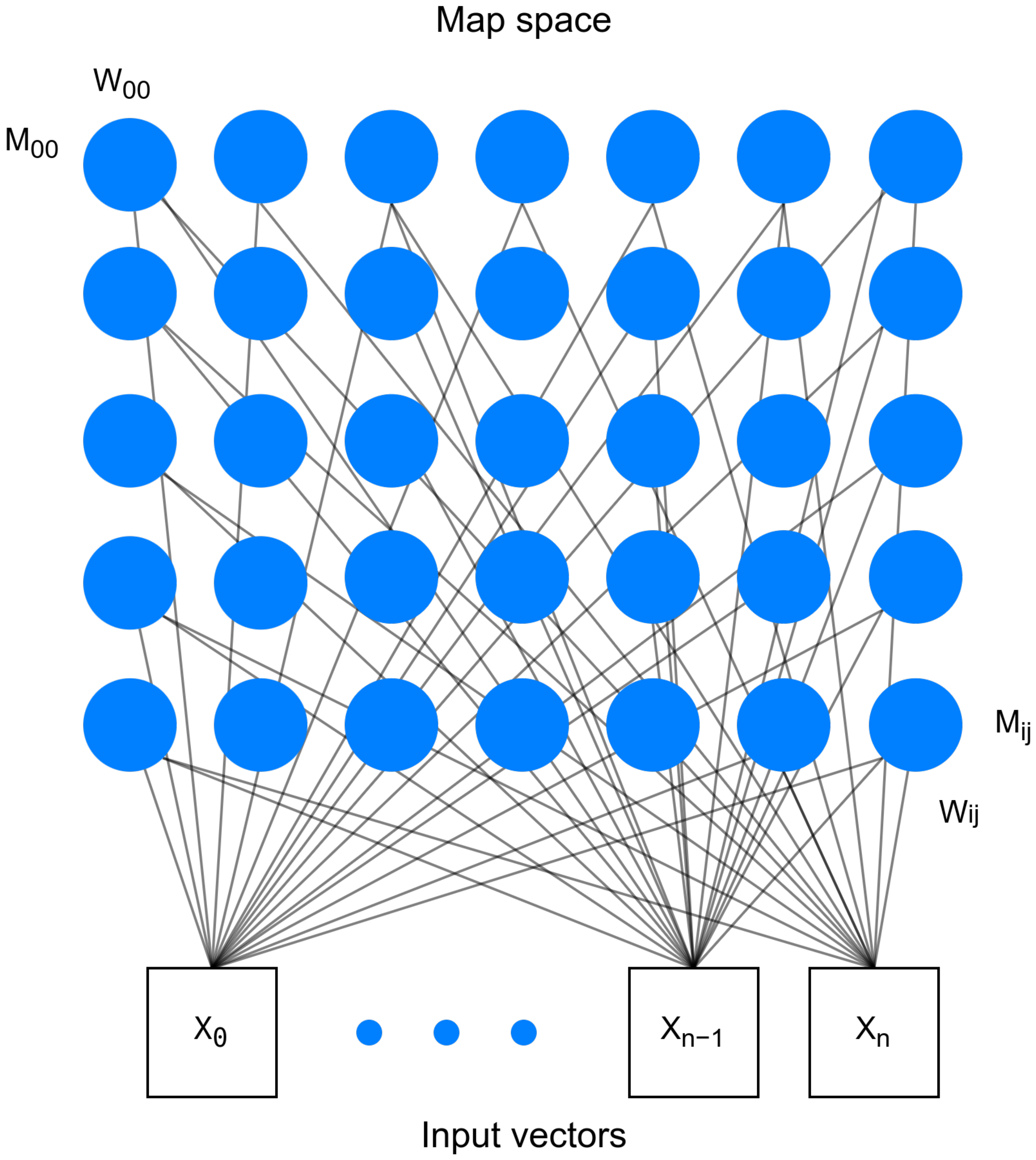
2. Self-Organizing Map

We describe the SOM in detail to establish a fundamental understanding of the proposed model. SOM is a competitive learning model that reduces the high-dimensional data to 2D maps, providing competent insight by combining similar data in a well-organized manner. The structure of SOM includes a fully connected input layer and map space (Figure 1). The predefined number of neurons $\left(M_{ij}\right)$ in the map space is arranged in a rectangular or hexagonal grid. The input vector $\left(X_n\right)$ and the neurons in the map space are associated with a weight vector $\left(W_{ij}\right)$. Random values ranging between 0 and 1 are assigned to the weight vectors to initialize the training. The dimension of the weight vector is the same as the dimension of the input vector. With each iteration of learning, the weight vector gets updated. The neurons in the map space stay fixed while the weight vectors move close to the input vector during the training process. The map orients itself adaptively to develop distinct classes of input vectors. During the learning of the SOM, various regions of the network respond similarly to specific input patterns. To find the best matching unit (BMU), the chosen input vector in the current iteration is compared to the neurons’ weight vector in the map space. The neuron with the closest distance measure to the input vector is selected as the BMU $\left(N_r\right)$. The frequently used distance measure is the Euclidean distance.

$$\begin{array}{c}\hfill distance,d=\sqrt{\sum _{k=1}^n{\left(x_r-w_k\right)}^2}\end{array}$$

(1)

where the total number of neurons in the map space is n. The $x_r$ is the randomly selected neuron.

The learning rate $\alpha \left(t\right)$ and the neighborhood radius $\sigma \left(t\right)$ are decaying values that slowly converge as the iteration progresses, and the following equations are used to compute them.

$$\alpha \left(t\right)={\alpha }_0\exp \left(-\frac{T}{\lambda }\right)$$

(2)

$$\sigma \left(t\right)={\sigma }_0\exp \left(-\frac{T}{\delta }\right)$$

(3)

where $\lambda$ and $\delta$ are the total number of epochs and the time constant, respectively. T is the current iteration value. ${\alpha }_0$ and ${\sigma }_0$ are the initial values of the learning rate and neighborhood radius. The SOM utilizes the Gaussian function to modify the weight vectors of the neighboring neurons (Figure 2). With the neighborhood influence, the weight vector of the neurons in the closer vicinity of the BMU is altered to become more identical to the BMU’s weight vector. The 2D map reaches equilibrium with successive training. For instance, the repeated occurrence of obtaining the same BMU does not affect the neighboring neurons’ weight vector in the 2D map. This feature facilitates SOM to alter itself only when it receives new input vectors. Significantly, with the unknown input vectors, the SOM can be retrained. The final 2D map adjusts itself to adapt to the newly presented input vectors. The fundamental SOM algorithm is shown in Algorithm 1.

Algorithm 1 Self-Organizing Map

INIT Map Size, $M_{ij}\leftarrow 10\times 10$

SET ∀ Weight Vectors, $W_{ij}\leftarrow$ Random values between 0 and 1

SET Learning rate, $\alpha \leftarrow 0.25$

SET Neighborhood radius, $\sigma \leftarrow 2.0$

SET Maximum iteration, $p\leftarrow 1000$

while  $k<p$  do

$X_r\leftarrow$ random input vector

Winner Neuron $N_c\leftarrow \mathit{find} \mathit{BMU}\left(X_r\right)$

$\alpha \left(t\right)\leftarrow \mathit{find} \mathit{decaying} \mathit{learning} \mathit{rate}\left(N_c\right)$

$\sigma \left(t\right)\leftarrow \mathit{find} \mathit{decaying} \mathit{neighborhood} \mathit{radius}\left(N_c\right)$

$h_{c,k}\left(t\right)\leftarrow \mathit{find} \mathit{neighborhood} \mathit{influence}\left(N_c\right)$

$w_r(t+1)\leftarrow \mathit{update} \mathit{weight} \mathit{vectors}\left(W_{ij}\right)$

end while

The neighborhood influence $h_{c,k}\left(t\right)$ is defined as,

$$h_{c,k}\left(t\right)=\exp \left(-\frac{d^2}{2·{\sigma }^2\left(t\right)}\right)$$

(4)

where $distance$ is computed using Equation (1). The computed learning rate, neighborhood influence, and previous weight matrix are utilized to update the current weight matrix.

$$w_r(t+1)=w_r\left(t\right)+\alpha \left(t\right)·h_{c,k}\left(t\right)·\left(x\left(t\right)-w_r\left(t\right)\right)$$

(5)

In the above equation, $w_r\left(t\right)$ is the weight vector of the randomly selected input vector at iteration t, $\alpha \left(t\right)$ is the learning rate, $h_{c,k}$ is the neighborhood influence, and $x\left(t\right)$ is the input vectors. As a result of training, a 2D map with spatially clustered neurons is obtained.

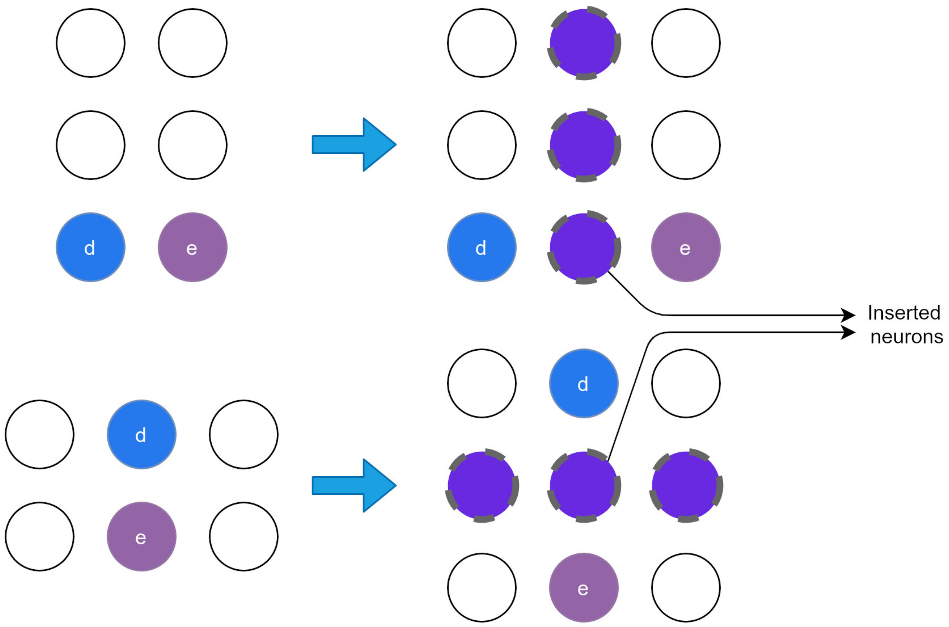
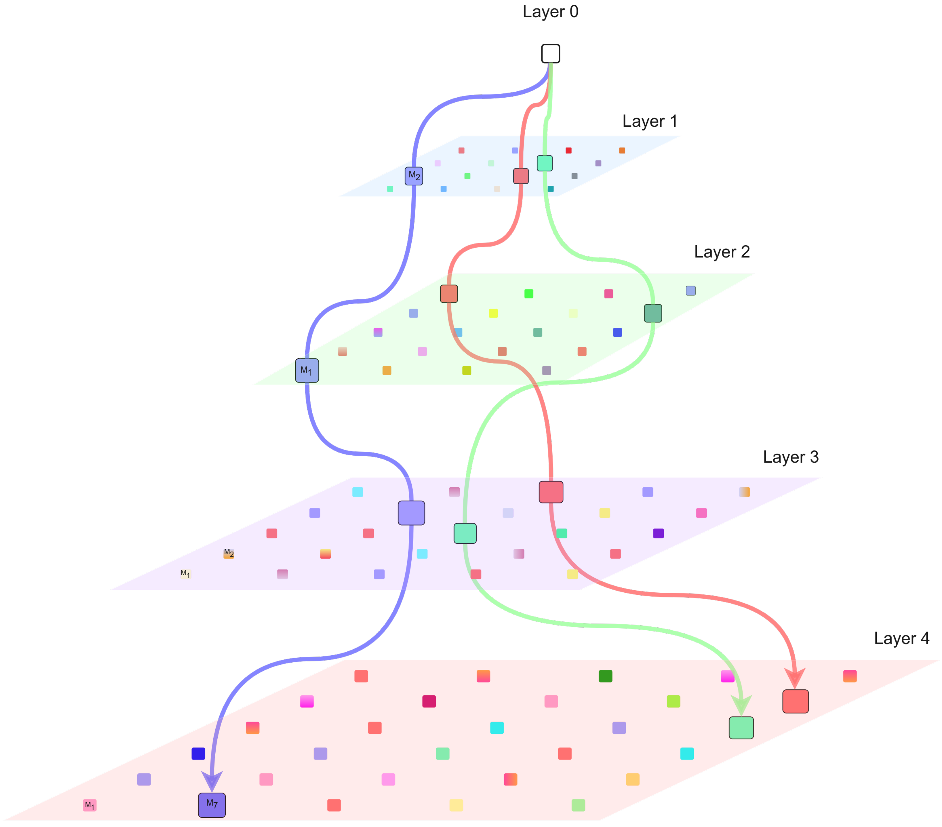
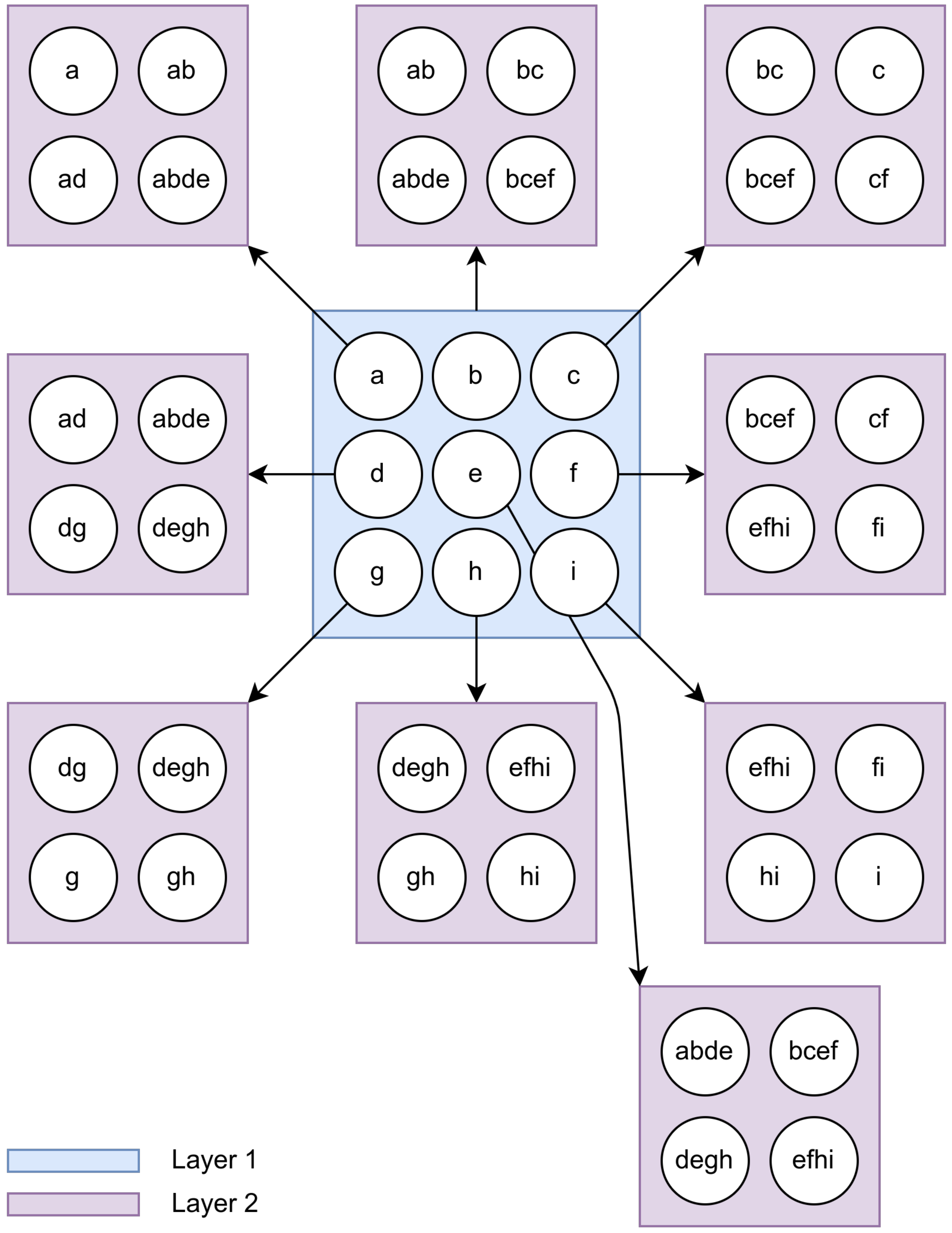
2.1. Growing Hierarchical Self-Organizing Map

Despite performing efficiently in unsupervised clustering, the SOM models require a prior definition of the map shape. Assistive robots often encounter unfamiliar problems with unprecedented uncertainties. The prior definition of objects, audio signals, and image data in the robot working environment is implausible. The robot architecture should update its knowledge base and adapt behavior based on newly discovered data. The static nature of standard SOM inhibits the exploration of a new association of knowledge building. The growing self-organizing maps (GSOM) [41] solve this problem by dynamically growing, but it tends to construct large maps for the enormous dataset. To overcome this shortcoming, growing hierarchical self-organizing maps (GHSOM) [42,54] have been proposed. The GHSOM model enables the large dataset to be clustered in hierarchical and horizontal ways, resulting in the effective decomposition of data. In GHSOM, the hierarchical structure has multiple layers, each with numerous independent growing SOMs. Each layer grows hierarchically until the hierarchical growing coefficient ${\tau }_2$ is reached. Similarly, each layer’s maps grow until the map growing coefficient ${\tau }_1$ is achieved. The starting process of the hierarchical growth depends on the overall deviation of the input vectors, computed as the mean of input vectors in the single-neuron zeroth layer.

$$mq{e}_0=\frac{1}{x_t}·\sum \parallel w_0-x_{map}\parallel$$

(6)

where $x_t$ is the total number of input vectors. $w_0$ is the weight vector of the single neuron in the zeroth layer. $x_{map}$ represents the input vector assigned for the zeroth neuron. The mean quantization error (MQE) is computed for each neuron to determine the growth of the child layer. The MQE of each neuron i is computed using the mean Euclidean distance between the neuron weight vector $w_i$ and its input vectors $x_i$.

$$mq{e}_i=\frac{1}{x_t}·\sum \parallel w_i-x_i\parallel$$

(7)

The MQE of each neuron in the map should be smaller than the product of hierarchical growing coefficient ${\tau }_2$ and $mq{e}_0$ to stop from growing.

$$mq{e}_i<{\tau }_2·mq{e}_0$$

(8)

when the neuron fails to satisfy conditions in Equation (8), the child map with 2 × 2 neurons is created for further data disintegration. The new child map will be initialized with random weight vectors. With the new child map, the training process follows the standard SOM training procedure. Once the training is complete, the MQE of all neurons will be computed. The dissimilarity in the data results in a high MQE, requiring new neurons for further clustering of the input vectors. Thus, the neuron with the highest MQE is taken as the error neuron e. From the current map, the most dissimilar neuron d is selected using the Euclidean distance measure. Based on the location, a new row or column of neurons is inserted between the error neuron e and its most dissimilar neighbor d (Figure 3).

The neighbors’ average will be selected as the weight vectors of the newly inserted neurons. After inserting new neurons, the current map will be retrained for the given number of iterations. The growth of a single map will be defined using the following condition.

$$MQ{E}_c<{\tau }_1·mq{e}_u$$

(9)

where $mq{e}_u$ is the $mqe$ of the current neuron u in the upper layer. The map growing coefficient ${\tau }_1$ helps limit the growth of the single map. The GHSOM structure resulting in a separation of clusters mapped onto different branches is shown in Figure 4 [55].

2.2. Parameter-Less Growing Hierarchical Self-Organizing Map

Although the GHSOM model efficiently clusters enormous data, it requires user-defined parameters such as learning rate and neighborhood radius for training. Since there is no specific analytical model to determine these parameters, the initial values are defined empirically.

Using the decaying learning rate and neighborhood radius eliminates the adaptability of the GHSOM model. Since these parameters follow the iteration-based decaying process, the GHSOM model fails to learn new information after the completion of the training. The parameter-less self-organizing map (PLSOM) is proposed [56,57] for the GHSOM model to overcome the shortcomings mentioned above. The significant distinction between PLSOM and the conventional SOM is that the PLSOM computes the learning rate and neighborhood size values on each iteration based on the error of the map to the input vector. This, in turn, allows the model to make substantial adjustments of these parameters to the unknown input vectors and tiny modifications to the learned input vectors. In the PLSOM, the weight matrix updates are not the function of the iteration number but, rather, the measure of how well the input vector fits the PLSOM. To identify the fitness, the scaling variable $\left(ϵ\right)$ is computed and applied to update the weight matrix. The $ϵ\left(t\right)$ is the normalized Euclidean distance from the input vector at time t to the weight vector of the BMU.

$$ϵ\left(t\right)=\frac{\parallel x\left(t\right)-w_{bmu}{\left(t\right)\parallel }_2}{p\left(t\right)}$$

(10)

$$p\left(t\right)=\max \left(\parallel x\left(t\right)-w_{bmu}{\left(t\right)\parallel }_2,\hspace{1em}p(t-1)\right)$$

(11)

$$p\left(0\right)=\parallel x\left(0\right)-w_{bmu}{\left(0\right)\parallel }_2$$

(12)

The scaling variable $ϵ$ is used to compute the neighborhood radius in the PLSOM.

$$\sigma \left(ϵ\left(t\right)\right)=(\beta -{\theta }_{min})\ln (1+ϵ\left(t\right)(e-1))+{\theta }_{min}$$

(13)

where $sigma\left(ϵ\right(t\left)\right)$ is the neighborhood radius from the scaling variable, e is the Euler number, $\beta$ is 2, and ${\theta }_{min}$ is 1. Using Equation (13), the neighborhood function and the weight updation is computed as follows.

$$h_{c,k}\left(t\right)=\exp \left(-\frac{d^2}{\sigma {\left(ϵ\left(t\right)\right)}^2}\right)$$

(14)

$$w_r(t+1)=w_r\left(t\right)+ϵ\left(t\right)·h_{c,k}\left(t\right)·\left(x\left(t\right)-w_r\left(t\right)\right)$$

(15)

From Equations (10) and (14), the PLSOM can update the weight matrix, eliminating iteration-based decaying. The variable $p\left(t\right)$ achieves its maximum value within a few iterations and will not change. Incorporating PLSOM with the GHSOM results in PL-GHSOM, where each layer in the hierarchy utilizes the PLSOM algorithm to compute the learning rate and neighborhood influence while training. When a neuron in the hierarchy expands, it creates an uninitialized 2 × 2 map in the subsequent layer. To establish a global orientation, the child map must be initialized with weight vectors that mimic the orientation of the neighboring neurons of its parent neuron. To achieve this, the fraction of weight vectors of the neighboring neurons of the parent neuron is added to the newly initialized map. Figure 5 shows the mapping of weight vectors to the newly created map.

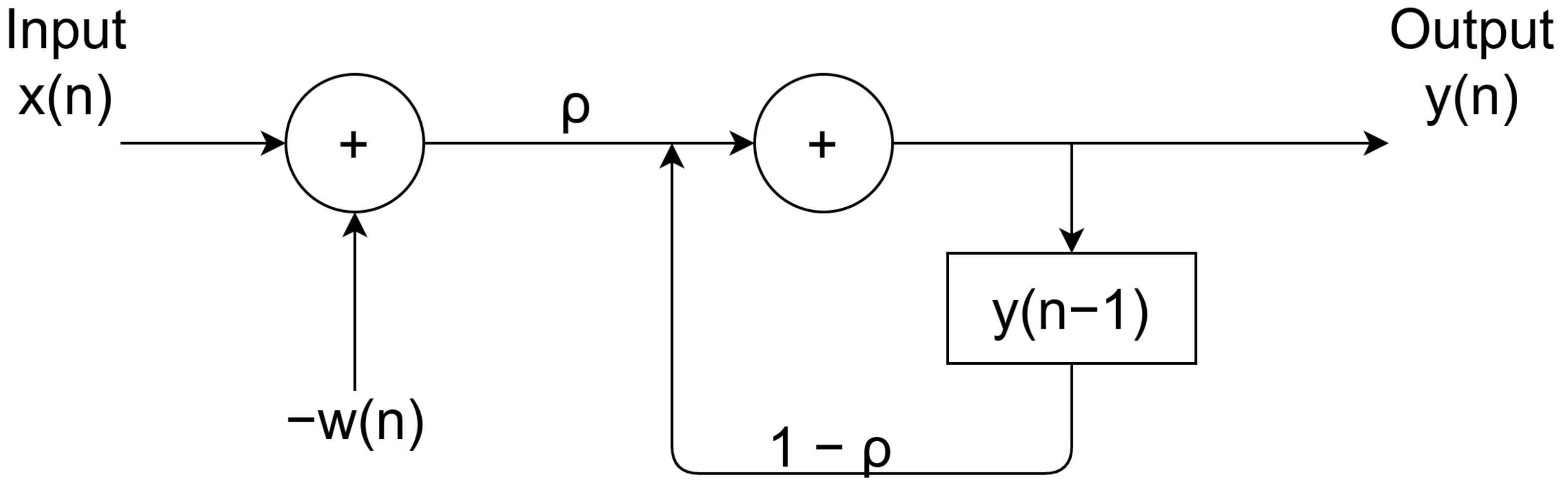
2.3. Recurrent Self-Organizing Map

Although the adaptive nature of the PL-GHSOM eliminates user intervention throughout the hierarchical training process, the model does not have any contextual knowledge about the input vectors, leading to inaccuracies in the problems involving time-series data. The recurrent self-organizing map (RSOM) model [58,59,60] is added to the PL-GHSOM to overcome this limitation. The RSOM incorporates the temporal knowledge of the input vectors both in determining BMU and weight matrix adaptation. To solve the temporal incorporation, a recursive difference equation is used for each neuron i in the map to determine the difference vector $y_i\left(t\right)$ for the given input vector $x\left(t\right)$ at time t (Figure 6).

$$y_i\left(t\right)=(1-\rho )·y_i(t-1)+\rho (x\left(t\right)-w_i\left(t\right))$$

(16)

where $\rho$ is the recursive coefficient deciding the influence of memory, and its value is $0<\rho \le 1$. When $\rho$ is closer to 1, the difference vector results in short-term memory; similarly, when $\rho$ is closer to 0, it represents long-term memory. The equation for updating the weight matrix of RSOM is similar to standard SOM weight updation but replaces $x\left(t\right)-w_i\left(t\right)$ with Equation (16). When applying $\rho =1$ in Equation (16), it produces the standard SOM weight updation. In Equation (17), the $\alpha \left(t\right)$ is the learning rate and $h_{c,k}\left(t\right)$ is neighborhood influence. At each learning cycle, a predefined number of previous input vectors are considered for the training, thereby learning contextual knowledge.

$$w_i(t+1)=w_i\left(t\right)+\alpha \left(t\right)h_{c,k}\left(t\right)y_i\left(t\right)$$

(17)

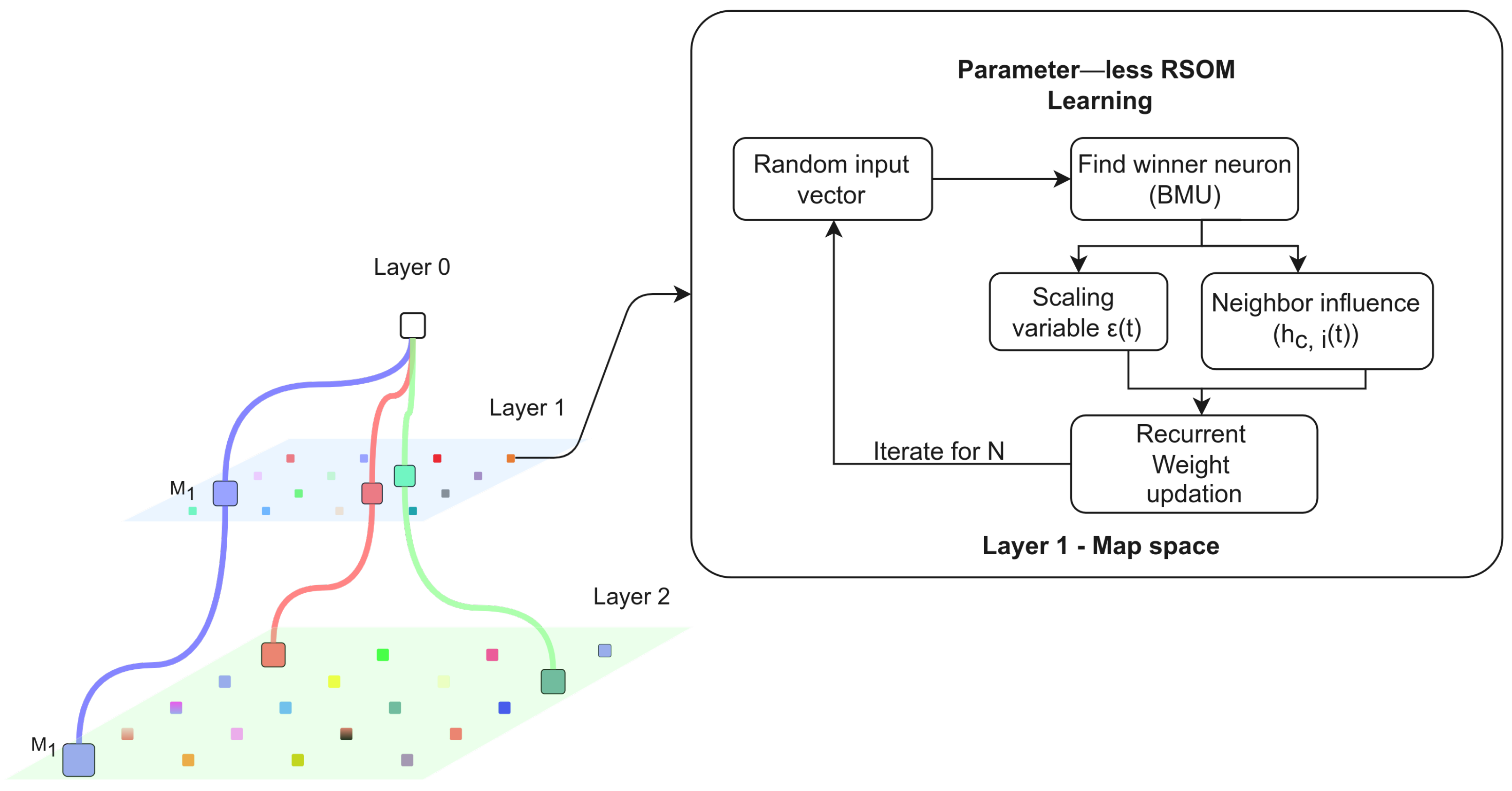
2.4. Parameter-Less Growing Hierarchical Recurrent Self-Organizing Map

Temporal memory is essential in decision making and knowledge building in the human brain. To imitate human-like learning, robot architecture must consider the temporal memory in the computation. Furthermore, the architecture should allow the robot to perceive distinct input parameters for decision making and knowledge building with a generalized computational model. To enable the inclusion of temporal knowledge and adaptive decision making, the PL-GHRSOM model has been proposed (Figure 7). The combination of RSOM and PL-GHSOM results in the generalized PL-GHRSOM model that efficiently clusters the distinct inputs based on temporal knowledge. The merging of the RSOM with the PL-GHSOM is accomplished by employing the RSOM’s difference equation and weight matrix updation to train each growing SOM model in the hierarchy.

The PL-GHRSOM model holds the contextual knowledge of the data in memory during learning, leading to an efficient understanding of time-series data. The PL-GHRSOM model eliminates the prior definition of the learning rate and neighborhood radius from the computation. The only parameters expected by the PL-GHRSOM model are the map growing coefficient and the hierarchical growing coefficient to regulate the horizontal and vertical growth of the hierarchy.

3. Testing and Evaluation

The two variants of the SOM models discussed in this paper are implemented as an open-source library. The library utilizes parallel computation to accelerate the training process of the maps in the hierarchy, resulting in significantly reduced computation time. The proposed models are examined and evaluated through various tasks such as unsupervised color clustering, handwritten digits clustering, finger identification, and image classification. These tasks help assistive robots better understand and interpret the visual information they receive from their environment. Color clustering identifies objects of interest, such as doors or pathways, while handwritten digit clustering allows the robot to recognize and interpret human-written information such as phone numbers. Finger recognition enables human users to communicate with the assistive robot using hand gestures. Image classification allows the robot to categorize objects in its working environment.

The resulting map will be huge for the smaller value of the map growing coefficient ${\tau }_1$, presenting the input data at a higher granularity. When ${\tau }_1$ is set to a larger value, the model creates a deeper hierarchy to represent the data further down the order. Each map in the hierarchy explains a distinct cluster of features of its input data. The depth/shallowness of the resulting hierarchical map can be controlled using ${\tau }_1$. Similarly, ${\tau }_2$ directly influences the overall size of the map space for data representation. The number of epochs for all experiments was set to 15. The values of ${\tau }_1$ and ${\tau }_2$ were selected empirically and set to 0.01 and 0.0001, respectively.

The simulation started with data preparation. The entire input dataset was split into train and test data. The input image vectors are converted to single-channel gray-scale images for the vision-based experiments since the proposed models’ implementation accepts only a 2D array as an input vector. The child neuron maps were trained using parallel processing to minimize computational time. The training was executed on the Ubuntu 20.04 with AMD Ryzen 9 3900x 12 core processor, 32 GB RAM, and 6 GB of NVIDIA Geforce RTX 2060 graphical processing unit. The first step in training was to initialize the zeroth map with parameters, including input vectors, total epoch ${\tau }_1$, and ${\tau }_2$. During training, neurons in the initial few hierarchies take ample time due to the dense nature of input vectors. As the training progresses, the lower-order hierarchies receive minimal compact data, thus resulting in reduced training time. We obtained a zeroth map from the training containing the neuron matrix. Each child map originated from the neurons in the zeroth map, forming a hierarchy. The implemented library allows the interactive navigation of the trained hierarchy. The initial interactive map shows the zeroth layer of the hierarchy and generates child maps based on the user’s mouse clicks. The mean vector of each map is computed using the following Equation.

$$M_{ij}=\frac{1}{N_{ij}}\sum _{k=1}^{N_{ij}}{W}_k$$

(18)

where $M_{ij}$ represents the mean vector of each map in the hierarchy. $N_{ij}$ represents the number of neurons in the map, and $W_k$ is the weight vector of the $k^{th}$ neuron.

The test images were new and unseen images for the models. The dimension of the neuron weight vector of each map in the hierarchy was the same as the input vector. The evaluation steps of the proposed models are as follows.

• Compute the mean vector of each map in the hierarchy (Equation (18)).
• Compare the test image with the maps in the hierarchy.
• Find the map with the closest mean vector for the test image.

The potential match is the map’s mean vector with the minimum Euclidean distance to the test vector.

Table 1. Comparison of results of different experiments for the SOM variants.

Test Type	GHSOM	GHRSOM	PL-GHSOM	PL-GHRSOM
Color Clustering	96.12%	96.03%	95.87%	95.98%
Handwritten Digits Clustering	92.62%	94.52%	95.09%	95.06%
Finger Identification	97.96%	97.89%	97.86%	97.84%
Image Classification	91.03%	91.06%	90.89%	90.69%

presents the results of the color clustering, handwritten digits clustering, finger identification, and image classification for the proposed models.

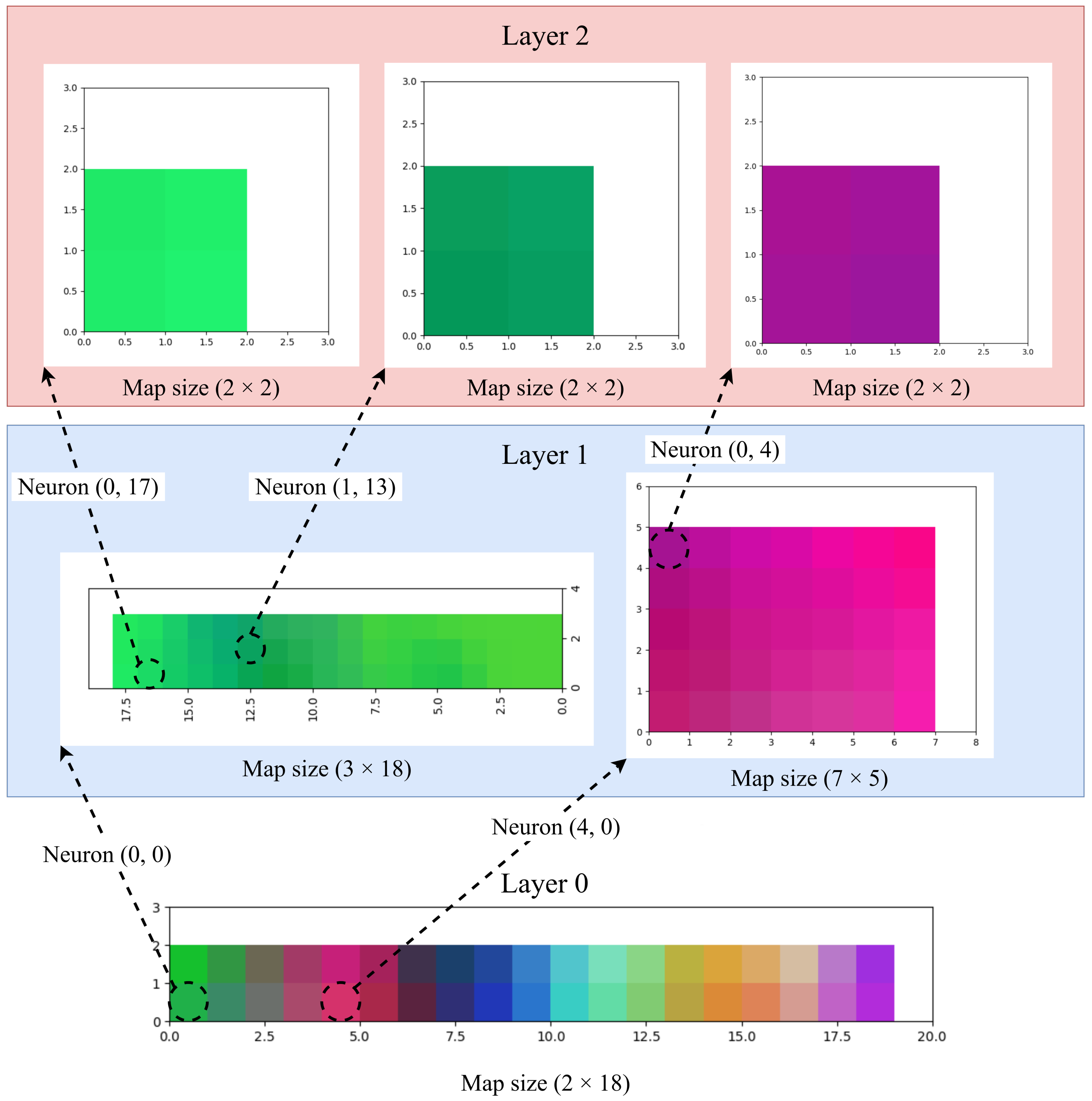
3.1. Color Clustering

A randomly generated RGB color data vector was used for the hierarchical color clustering and evaluation. Each data point consisted of three features from 0 to 1, representing RGB values. The training started with the initialization of the zeroth neuron.

The model expands the current map from the input vectors by adding neuron layers. Likewise, the neurons that require hierarchical branching grow further as a new map layer. The training process follows the batch training procedure. The selected batch of input vectors is given as input to the proposed SOM variants. The PL-GHSOM employs PLSOM learning models to train maps in the hierarchy, while the PL-GHRSOM utilizes PLRSOM models. The resulting hierarchical maps contain similar input vectors clustered together as individual color maps (Figure 8).

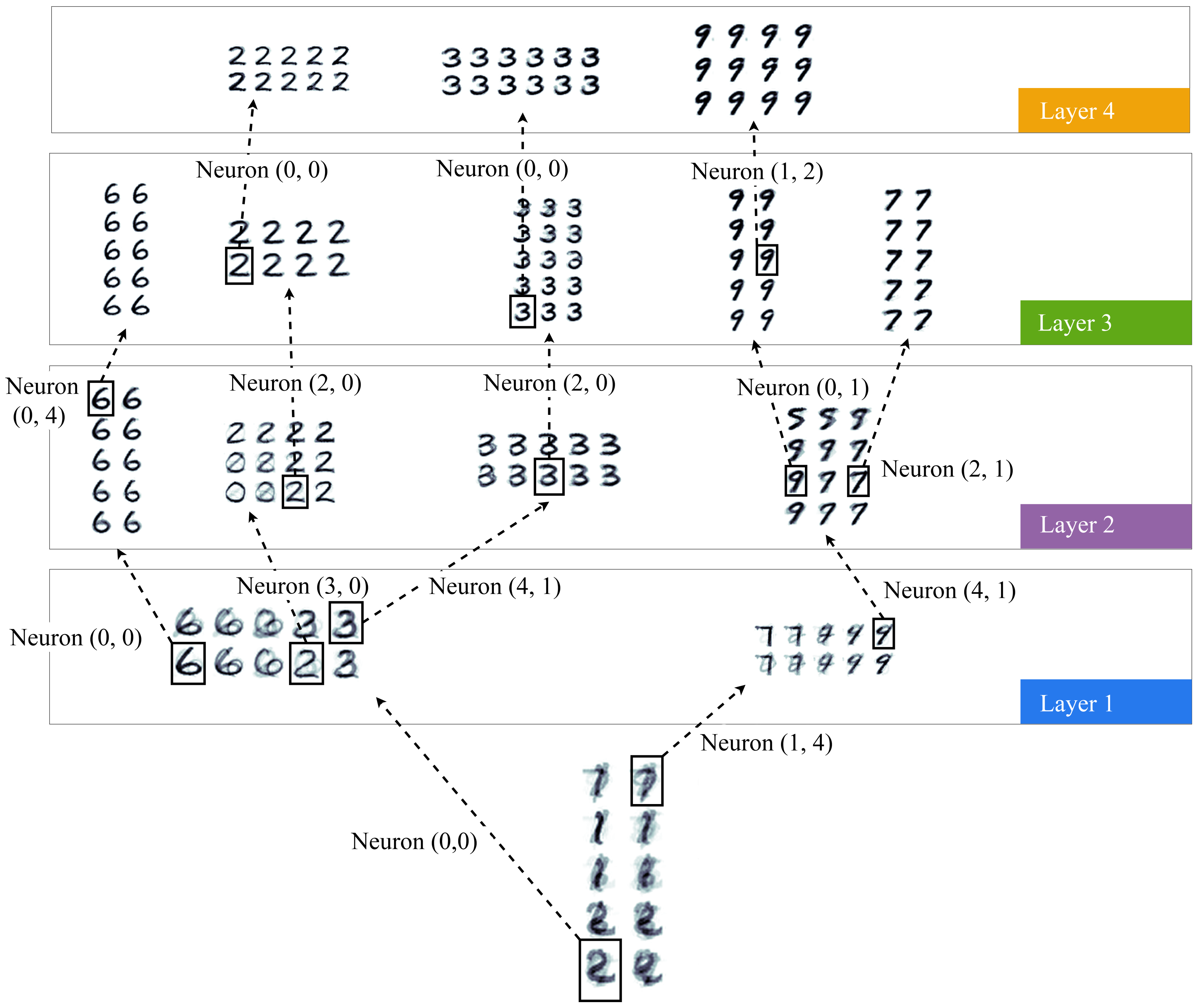
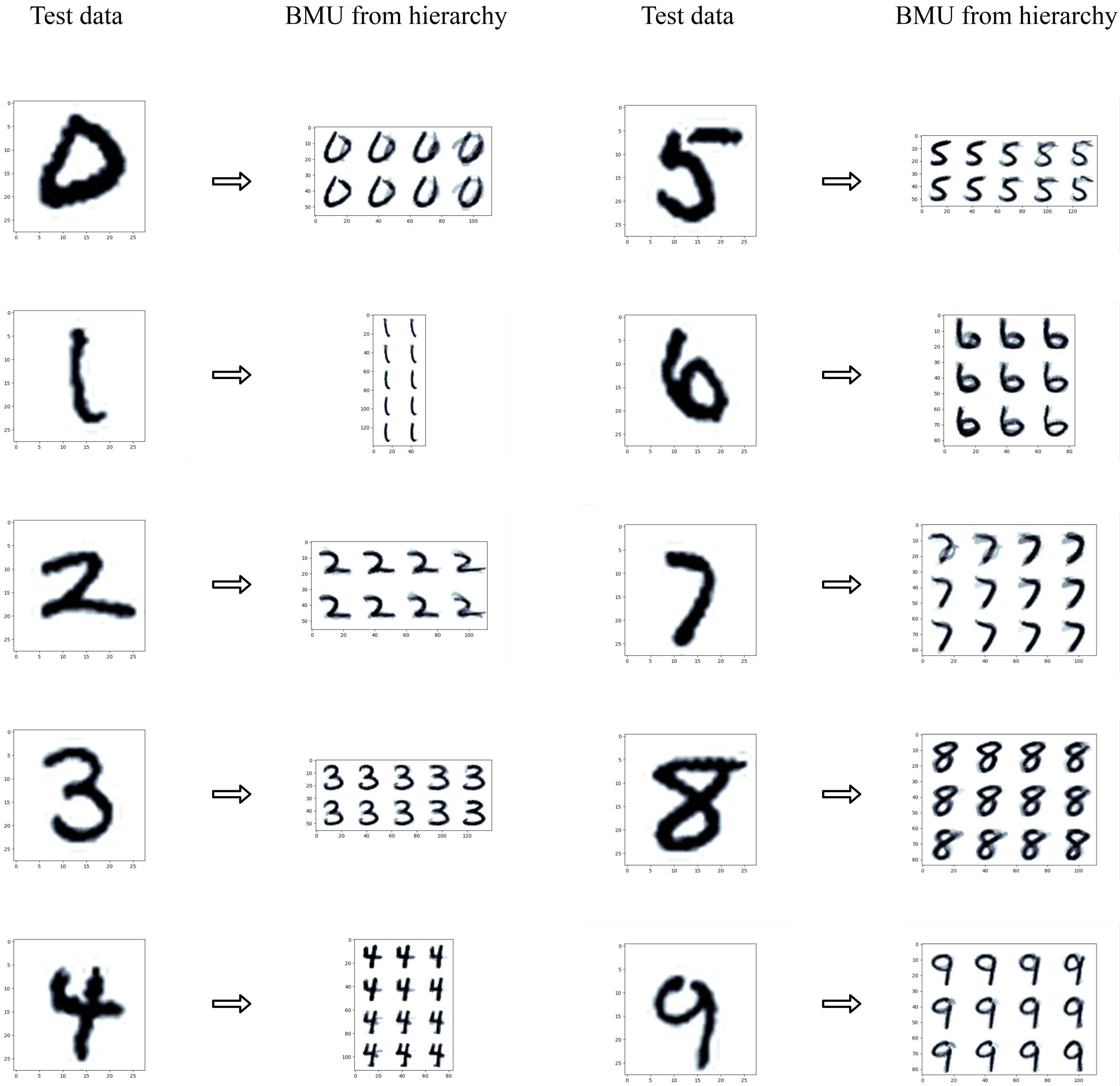
3.2. Handwritten Digits Clustering

The MNIST handwritten digit dataset was used for digit clustering. The overall dataset contains 70,000 images of handwritten digits. The data was divided into 59,500 training samples and 10,500 test samples. The images in the MNIST dataset contain a grayscale value of 28 × 28 pixels. The subsequent layers in the hierarchy are shown in Figure 9. The best matching maps from the hierarchy for each test vector are shown in Figure 10.

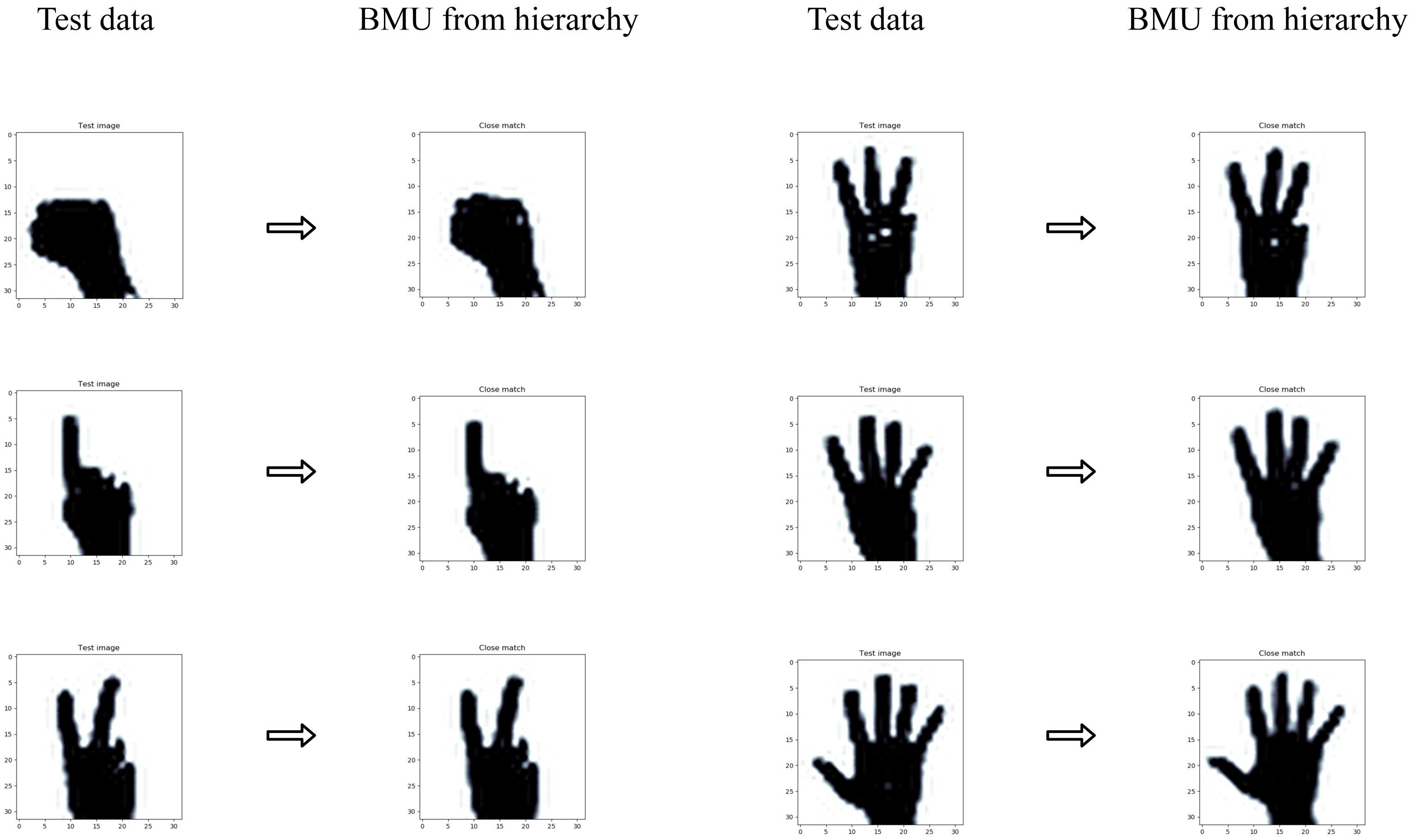
3.3. Finger Identification

To test the performance of the proposed models, the finger-counting problem was selected. The finger count was identified from the input image using the trained model. The evaluation was conducted on a set of 12,006 images depicting a hand holding up between 0 and 5 fingers. The dataset was divided into 9604 training images and 2402 test images using the “train-test-split” function from scikit-learn library [61]. The function utilizes the “sampling without replacing” method to split the data into training and test data. Each image in the dataset contains 128 × 128 pixels. The map growing and Hierarchical growing coefficients were set to 0.1 and 0.0001, as before. Figure 11 shows the best matching image from the hierarchy for each test image. The map with the closest mean vector was chosen as the final map. Again, from the resulting map, the image with the closest mean distance was selected as the output image.

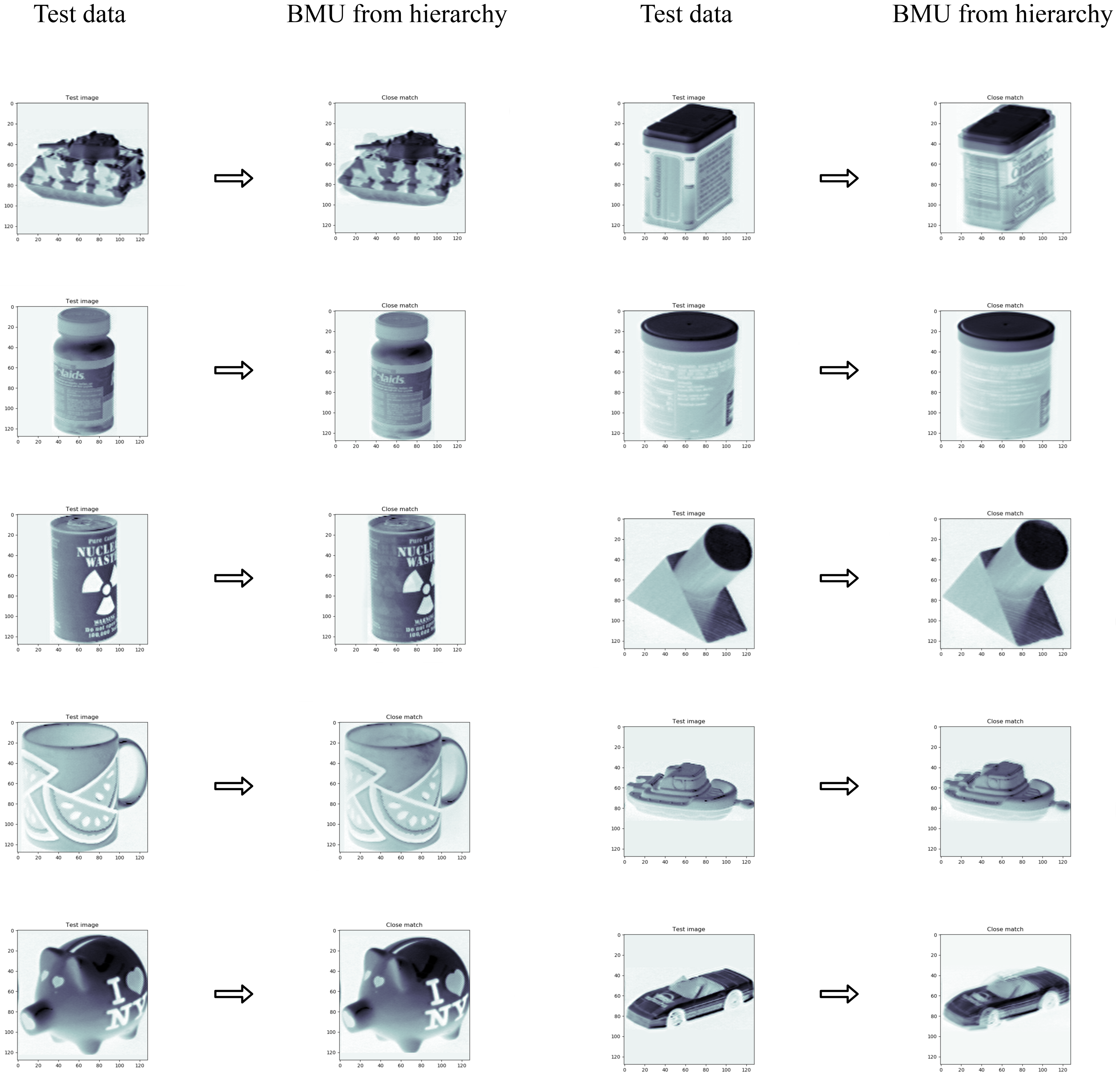
3.4. Object Classification

For the final evaluation, the model was presented with the object classification problem. COIL-100 data were used for the analysis. The dataset contains 100 images of objects taken from angles ranging from 0 to 355 degrees, with an interval of 5 degrees. The dataset consists of 7200 images with a wide variety of complex geometry and reflectance properties. The dataset was split into 5760 training images and 1440 test images. Each image has a resolution of 128 × 128 pixels. The best matching map for each test data is shown in Figure 12.

4. Conclusions

The computational models used in assistive robots for decision making are data driven, requiring an extensive labeled dataset to build their knowledge base. This prerequisite is counter-intuitive to the infant learning model. This paper presented two unsupervised SOM variants, PL-GHSOM and PL-GHRSOM, to imitate infant learning. An in-depth explanation of the algorithms and their implementation methodologies was discussed. The extensive testing and evaluation exhibit that the proposed models acquire knowledge patterns without prior knowledge, which is indispensable for assistive robots. The models also require minimal inputs from humans to learn. The presented models are great at interpolation and are unaffected by the absence of data vectors. For instance, the models are trained with data vectors with a set of angles in the object classification example. However, for the test vector with a distinct angle, the model predictions are undoubtedly close to the original image. Each map in the hierarchy constantly adapts itself to match the corresponding input vectors. This adaptive behavior enables the model to produce new patterns not present in the input vectors. The PL-GHSOM and PL-GHRSOM are competent in processing distinct inputs from their environment without modification. Consequently, the choice of these models as the generalized computational model provides improved adaptability and human-like learning to assistive robots. The primary advantage of the presented models is that they can uncover the indiscernible hierarchical structure in the input data without predefined parameters and human supervision.

Though the proposed models perform well on clustering unsupervised data, two shortcomings limit the models. The standard SOM allows retraining the trained map with the newly received inputs, leading to adaptive learning. However, the proposed models lack retraining capability, i.e., when the new input vectors are presented, the entire model needs to be retrained to include the influence of the unknown input vectors. To address this limitation, one possible method is to compare the new input vectors with the trained hierarchy and include them in the map with the closest mean vector. However, if an input vector does not match the mean vectors of any maps in the hierarchy, a new map should be created under the zeroth layer to accommodate all unknown input vectors.

The second limitation is that the model lacks the association layer to form the link between two different problems, i.e., the model can learn two distinct problems separately, while it cannot develop connections between them. Johnsson [62] proposed a new variant of SOM named associative self-organizing map (ASOM) that contains a separate map to link the association among distinct SOM models. The dynamically growing ASOM model can be incorporated into the proposed models to form associations among different maps in the hierarchy.

The retraining capability and associative learning are the future expected outcomes of this study. The proposed models are tested and evaluated in the simulated environment. Future research will assess the proposed models’ functioning and capabilities by applying them to a physical robot.

References

1. Johnson, D.O.; Cuijpers, R.H.; Juola, J.F.; Torta, E.; Simonov, M.; Frisiello, A.; Bazzani, M.; Yan, W.; Weber, C.; Wermter, S.; et al. Socially Assistive Robots: A Comprehensive Approach to Extending Independent Living. Int. J. Soc. Robot. 2014, 6, 195–211. [Google Scholar] [CrossRef]
2. Matarić, M.J.; Scassellati, B. Socially assistive robotics. In Springer Handbook of Robotics; Springer: Berlin/Heidelberg, Germany, 2016; pp. 1973–1994. [Google Scholar]
3. Maslach, C.; Leiter, M.P. Understanding burnout: New models. In The Handbook of Stress and Health: A Guide to Research and Practice; John Wiley & Sons Ltd.: West Sussex, UK, 2017; pp. 36–56. [Google Scholar]
4. Bianchi, R.; Boffy, C.; Hingray, C.; Truchot, D.; Laurent, E. Comparative symptomatology of burnout and depression. J. Health Psychol. 2013, 18, 782–787. [Google Scholar] [CrossRef] [PubMed]
5. Bemelmans, R.; Gelderblom, G.J.; Jonker, P.; de Witte, L. Socially Assistive Robots in Elderly Care: A Systematic Review into Effects and Effectiveness. J. Am. Med Dir. Assoc. 2012, 13, 114–120.e1. [Google Scholar] [CrossRef]
6. Dickstein-Fischer, L.A.; Crone-Todd, D.E.; Chapman, I.M.; Fathima, A.T.; Fischer, G.S. Socially assistive robots: Current status and future prospects for autism interventions. Innov. Entrep. Health 2018, 5, 15–25. [Google Scholar] [CrossRef]
7. Ingrand, F. Deliberation for autonomous robots: A survey. Artificial Intell. 2017, 247, 10–44. [Google Scholar] [CrossRef]
8. Feng, F.; Chan, R.H.; Shi, X.; Zhang, Y.; She, Q. Challenges in task incremental learning for assistive robotics. IEEE Access 2019, 8, 3434–3441. [Google Scholar] [CrossRef]
9. Santhanaraj, K.K.; Ramya, M.M.; Dinakaran, D. A survey of assistive robots and systems for elderly care. J. Enabling Technol. 2021, 15, 66–72. [Google Scholar] [CrossRef]
10. Bousquet-Jette, C.; Achiche, S.; Beaini, D.; Cio, Y.L.K.; Leblond-Ménard, C.; Raison, M. Fast scene analysis using vision and artificial intelligence for object prehension by an assistive robot. Eng. Appl. Artif. Intell. 2017, 63, 33–44. [Google Scholar] [CrossRef]
11. Chollet, F. Xception: Deep learning with depthwise separable convolutions. In Proceedings of the IEEE Conference on Computer Vision and Pattern Recognition, Honolulu, HI, USA, 21–26 July 2017; pp. 1251–1258. [Google Scholar]
12. Montaño-Serrano, V.M.; Jacinto-Villegas, J.M.; Vilchis-González, A.H.; Portillo-Rodríguez, O. Artificial Vision Algorithms for Socially Assistive Robot Applications: A Review of the Literature. Sensors 2021, 21, 5728. [Google Scholar] [CrossRef]
13. Panek, P.; Mayer, P. Challenges in adopting speech control for assistive robots. In Ambient Assisted Living; Springer: Berlin/Heidelberg, Germany, 2015; pp. 3–14. [Google Scholar]
14. Li, J. Recent Advances in End-to-End Automatic Speech Recognition. APSIPA Trans. Signal Inf. Process. 2022, 11, e8. [Google Scholar] [CrossRef]
15. Wang, H.; Wang, C.; Xie, L. Intensity-slam: Intensity assisted localization and mapping for large scale environment. IEEE Robot. Autom. Lett. 2021, 6, 1715–1721. [Google Scholar] [CrossRef]
16. Ali, A.J.B.; Kouroshli, M.; Semenova, S.; Hashemifar, Z.S.; Ko, S.Y.; Dantu, K. Edge-SLAM: Edge-assisted visual simultaneous localization and mapping. ACM Trans. Embed. Comput. Syst. 2022, 22, 1–31. [Google Scholar] [CrossRef]
17. Elshaw, M.; Moore, R.K.; Klein, M. Hierarchical Recurrent Self-Organising Memory (H-RSOM) Architecture for an Emergent Speech Representation towards Robot Grounding. Available online: http://lands.let.ru.nl/acorns/documents/publications/NCAF_paper_2009.pdf (accessed on 8 May 2023).
18. Zhang, T.; Zeng, Y.; Pan, R.; Shi, M.; Lu, E. Brain-Inspired Active Learning Architecture for Procedural Knowledge Understanding Based on Human-Robot Interaction. Cogn. Comput. 2021, 13, 381–393. [Google Scholar] [CrossRef]
19. Gergely, G. What should a robot learn from an infant? Mechanisms of action interpretation and observational learning in infancy. Connect. Sci. 2003, 15, 191–209. [Google Scholar] [CrossRef]
20. Anderson, J.R.; Matessa, M.; Lebiere, C. ACT-R: A theory of higher level cognition and its relation to visual attention. Human–Comput. Interact. 1997, 12, 439–462. [Google Scholar] [CrossRef]
21. Ritter, F.E.; Tehranchi, F.; Oury, J.D. ACT-R: A cognitive architecture for modeling cognition. WIREs Cogn. Sci. 2019, 10, e1488. [Google Scholar] [CrossRef]
22. Rosenbloom, P.S. The Sigma cognitive architecture and system. AISB Q. 2013, 136, 4–13. [Google Scholar]
23. Ustun, V.; Rosenbloom, P.S.; Sajjadi, S.; Nuttall, J. Controlling Synthetic Characters in Simulations: A Case for Cognitive Architectures and Sigma. arXiv 2021, arXiv:2101.02231. [Google Scholar]
24. Rosenbloom, P.S.; Ustun, V. An architectural integration of Temporal Motivation Theory for decision making. In Proceedings of the 17th Annual Meeting of the International Conference on Cognitive Modeling, Montreal, QC, Canada, 19–22 July 2019. [Google Scholar]
25. Singer, W. The brain as a self-organizing system. Eur. Arch. Psychiatry Neurol. Sci. 1986, 236, 4–9. [Google Scholar] [CrossRef]
26. Singer, W. The Brain, a Complex Self-organizing System. Eur. Rev. 2009, 17, 321–329. [Google Scholar] [CrossRef]
27. Van Orden, G.C.; Holden, J.G.; Turvey, M.T. Self-organization of cognitive performance. J. Exp. Psychol. Gen. 2003, 132, 331–350. [Google Scholar] [CrossRef] [PubMed]
28. Dresp-Langley, B. Seven Properties of Self-Organization in the Human Brain. Big Data Cogn. Comput. 2020, 4, 10. [Google Scholar] [CrossRef]
29. Patel, M.; Miro, J.V.; Dissanayake, G. A hierarchical hidden markov model to support activities of daily living with an assistive robotic walker. In Proceedings of the 2012 4th IEEE RAS & EMBS International Conference on Biomedical Robotics and Biomechatronics (BioRob), Rome, Italy, 24–27 June 2012; IEEE: Manhattan, NY, USA, 2012; pp. 1071–1076. [Google Scholar]
30. Zhou, X.; Bai, T.; Gao, Y.; Han, Y. Vision-Based Robot Navigation through Combining Unsupervised Learning and Hierarchical Reinforcement Learning. Sensors 2019, 19, 1576. [Google Scholar] [CrossRef] [PubMed]
31. Sharma, A.; Ahn, M.; Levine, S.; Kumar, V.; Hausman, K.; Gu, S. Emergent real-world robotic skills via unsupervised off-policy reinforcement learning. arXiv 2020, arXiv:2004.12974. [Google Scholar]
32. Wang, C.; Qiu, Y.; Wang, W.; Hu, Y.; Kim, S.; Scherer, S. Unsupervised online learning for robotic interestingness with visual memory. IEEE Trans. Robot. 2021, 38, 2446–2461. [Google Scholar] [CrossRef]
33. Yates, T.S.; Ellis, C.T.; Turk-Browne, N.B. Emergence and organization of adult brain function throughout child development. NeuroImage 2021, 226, 117606. [Google Scholar] [CrossRef]
34. Haken, H. Synergetics of brain function. Int. J. Psychophysiol. 2006, 60, 110–124. [Google Scholar] [CrossRef]
35. Chersi, F.; Ferro, M.; Pezzulo, G.; Pirrelli, V. Topological Self-Organization and Prediction Learning Support Both Action and Lexical Chains in the Brain. Top. Cogn. Sci. 2014, 6, 476–491. [Google Scholar] [CrossRef]
36. Fingelkurts, A.A.; Fingelkurts, A.A.; Neves, C.F. Consciousness as a phenomenon in the operational architectonics of brain organization: Criticality and self-organization considerations. Chaos Solitons Fractals 2013, 55, 13–31. [Google Scholar] [CrossRef]
37. Lloyd, R. Self-organized cognitive maps. Prof. Geogr. 2000, 52, 517–531. [Google Scholar] [CrossRef]
38. Doniec, M.W.; Scassellati, B.; Miranker, W.L. Emergence of Language-Specific Phoneme Classifiers in Self-Organized Maps. In Proceedings of the 2007 International Joint Conference on Neural Networks, Orlando, FL, USA, 12–17 August 2007; pp. 2081–2086. [Google Scholar] [CrossRef]
39. Huang, K.; Ma, X.; Song, R.; Rong, X.; Tian, X.; Li, Y. An autonomous developmental cognitive architecture based on incremental associative neural network with dynamic audiovisual fusion. IEEE Access 2019, 7, 8789–8807. [Google Scholar] [CrossRef]
40. Kohonen, T. The self-organizing map. Proc. IEEE 1990, 78, 1464–1480. [Google Scholar] [CrossRef]
41. Alahakoon, D.; Halgamuge, S.; Srinivasan, B. Dynamic self-organizing maps with controlled growth for knowledge discovery. IEEE Trans. Neural Netw. 2000, 11, 601–614. [Google Scholar] [CrossRef] [PubMed]
42. Dittenbach, M.; Merkl, D.; Rauber, A. The growing hierarchical self-organizing map. In Proceedings of the IEEE-INNS-ENNS International Joint Conference on Neural Networks. IJCNN 2000. Neural Computing: New Challenges and Perspectives for the New Millennium, Como, Italy, 27–27 July 2000; IEEE: Manhattan, NY, USA, 2000; Volume 6, pp. 15–19. [Google Scholar]
43. Walker, A.; Hallam, J.; Willshaw, D. Bee-havior in a mobile robot: The construction of a self-organized cognitive map and its use in robot navigation within a complex, natural environment. In Proceedings of the IEEE International Conference on Neural Networks, San Francisco, CA, USA, 28 March–1 April 1993; pp. 1451–1456. [Google Scholar] [CrossRef]
44. Huang, K.; Ma, X.; Song, R.; Rong, X.; Tian, X.; Li, Y. A self-organizing developmental cognitive architecture with interactive reinforcement learning. Neurocomputing 2020, 377, 269–285. [Google Scholar] [CrossRef]
45. Huang, K.; Ma, X.; Song, R.; Rong, X.; Li, Y. Autonomous cognition development with lifelong learning: A self-organizing and reflecting cognitive network. Neurocomputing 2021, 421, 66–83. [Google Scholar] [CrossRef]
46. Gliozzi, V.; Madeddu, M. A visual auditory model based on Growing Self-Organizing Maps to analyze the taxonomic response in early childhood. Cogn. Syst. Res. 2018, 52, 668–677. [Google Scholar] [CrossRef]
47. Mici, L.; Parisi, G.I.; Wermter, S. An Incremental Self-Organizing Architecture for Sensorimotor Learning and Prediction. IEEE Trans. Cogn. Dev. Syst. 2018, 10, 918–928. [Google Scholar] [CrossRef]
48. Zhu, D.; Cao, X.; Sun, B.; Luo, C. Biologically Inspired Self-Organizing Map Applied to Task Assignment and Path Planning of an AUV System. IEEE Trans. Cogn. Dev. Syst. 2018, 10, 304–313. [Google Scholar] [CrossRef]
49. Jitviriya, W.; Hayashi, E. Design of emotion generation model and action selection for robots using a Self Organizing Map. In Proceedings of the 2014 11th International Conference on Electrical Engineering/Electronics, Computer, Telecommunications and Information Technology (ECTI-CON), Nakhon Ratchasima, Thailand, 14–17 May 2014; pp. 1–6. [Google Scholar] [CrossRef]
50. Jitviriya, W.; Koike, M.; Hayashi, E. Emotional Model for Robotic System Using a Self-Organizing Map Combined with Markovian Model. J. Robot. Mechatronics 2015, 27, 563–570. [Google Scholar] [CrossRef]
51. Johnsson, M.; Balkenius, C. Sense of touch in robots with self-organizing maps. IEEE Trans. Robot. 2011, 27, 498–507. [Google Scholar] [CrossRef]
52. LeCun, Y.; Bottou, L.; Bengio, Y.; Haffner, P. Gradient-based learning applied to document recognition. Proc. IEEE 1998, 86, 2278–2324. [Google Scholar] [CrossRef]
53. Nene, S.A.; Nayar, S.K.; Murase, H. Columbia Object Image Library (Coil-100); Citeseer: State College, PA, USA, 1996. [Google Scholar]
54. Rauber, A.; Merkl, D.; Dittenbach, M. The growing hierarchical self-organizing map: Exploratory analysis of high-dimensional data. IEEE Trans. Neural Netw. 2002, 13, 1331–1341. [Google Scholar] [CrossRef] [PubMed]
55. Dittenbach, M.; Rauber, A.; Merkl, D. Recent advances with the growing hierarchical self-organizing map. In Advances in Self-Organising Maps; Springer: Berlin/Heidelberg, Germany, 2001; pp. 140–145. [Google Scholar]
56. Berglund, E.; Sitte, J. The parameterless self-organizing map algorithm. IEEE Trans. Neural Netw. 2006, 17, 12. [Google Scholar] [CrossRef] [PubMed]
57. Kuremoto, T.; Komoto, T.; Kobayashi, K.; Obayashi, M. Parameterless-Growing-SOM and Its Application to a Voice Instruction Learning System. J. Robot. 2010, 2010, 307293. [Google Scholar] [CrossRef]
58. Varsta, M.; Heikkonen, J.; Millan, J.d.R. Context Learning with the Self-Organizing Map; Helsinki University of Technology: Espoo, Finland, 1997. [Google Scholar]
59. Angelovič, P. Time series prediction using RSOM and local models. In Proceedings of IIT.SRC 2005, Bratislava, Slovakia, 23 April 2015; Citeseer: State College, PA, USA, 2005; pp. 27–34. [Google Scholar]
60. Sá, J.; Rocha, B.; Almeida, A.; Souza, J.R. Recurrent self-organizing map for severe weather patterns recognition. Recurr. Neural Netw. Solf Comput. 2012, 8, 151–175. [Google Scholar]
61. Pedregosa, F.; Varoquaux, G.; Gramfort, A.; Michel, V.; Thirion, B.; Grisel, O.; Blondel, M.; Prettenhofer, P.; Weiss, R.; Dubourg, V.; et al. Scikit-learn: Machine learning in Python. J. Mach. Learn. Res. 2011, 12, 2825–2830. [Google Scholar]
62. Johnsson, M.; Balkenius, C.; Hesslow, G. Associative self-organizing map. In Proceedings of the International Conference on Neural Computation, Tianjin, China, 14–16 August 2009; SCITEPRESS: Setúbal, Portugal, 2009; Volume 2, pp. 363–370. [Google Scholar]
Figure 1. Initial self–organizing map structure. M i j represents neurons in the map space. W i j represents weight vectors of the corresponding neuron. X n represent the component of the input vector.
Make 05 00030 g001
Figure 2. Gaussian function-based neighborhood influence ( h c , k ( t ) ) for the Winner neuron ( N c ) .
Make 05 00030 g002
Figure 3. Insertion of new neurons between error neuron (e) and its most dissimilar neighbor neuron (d).
Make 05 00030 g003
Figure 4. Overview of growing hierarchical self-organizing map (GHSOM). M i represents the map in the n t h layer. The connection denotes the hierarchical expansion. Each connection consists of parent neuron and a child map.
Make 05 00030 g004
Figure 5. Data mapping of weight vectors to the newly created maps. The child neuron (purple) receives a fraction of the weight vectors of the neighboring neurons of the parent neuron (blue). For instance, the child neuron created from the parent neuron a receives its four neighboring neurons’ weight vectors namely a , a b , a d , a b d e .
Make 05 00030 g005
Figure 6. Block diagram of Recurrent Self-organizing Map.
Make 05 00030 g006
Figure 7. Block diagram of training of each map in the Parameter—less Growing Self-Organizing Map. Each map in the hierarchy utilizes recurrent learning. The connection in the hierarchy denotes the hierarchical expansion. Each connection consists of parent neuron and a child map.
Make 05 00030 g007
Figure 8. Interactive result of hierarchical color clustering. Each neuron’s weight vector represents RGB values.
Make 05 00030 g008
Figure 9. Interactive result of hierarchical handwritten digit clustering. Starting from the zeroth layer, the digits are precise and finite in the higher-order layers.
Make 05 00030 g009
Figure 10. Digits clustering—BMU for each test data from the hierarchy.
Make 05 00030 g010
Figure 11. Finger identification—best matching images from the hierarchy for the test images.
Make 05 00030 g011
Figure 12. Object classification—best matching images from the hierarchy for the test images. The model predicts the same object with a different angle from the BMU for the test image.
Make 05 00030 g012