Abstract
Representations from common pre-trained language models have been shown to suffer from the degeneration problem, i.e., they occupy a narrow cone in latent space. This problem can be addressed by enforcing isotropy in latent space. In analogy with variational autoencoders, we suggest applying a token-level variational loss to a Transformer architecture and optimizing the standard deviation of the prior distribution in the loss function as the model parameter to increase isotropy. The resulting latent space is complete and interpretable: any given point is a valid embedding and can be decoded into text again. This allows for text manipulations such as paraphrase generation directly in latent space. Surprisingly, features extracted at the sentence level also show competitive results on benchmark classification tasks.
1. Introduction
Self-supervised, attention-based language models are prone to overfitting or memorizing input data, especially when trained on smaller datasets. Nevertheless, models such as BERT [1], based on an encoder-only architecture and trained on very large datasets, exhibit state-of-the-art performance on common natural language processing tasks. The resulting token representations of these models are distributed and highly contextual, but the latent space does not exhibit additional structural properties such as isotropy and the resulting smoothness and completeness [2].
Previous work has shown that isotropic latent representations, which are distributed across latent space instead of populating a narrow cone [2], can improve the performance of language models on transfer tasks. Gao et al. [3] improved the performance of a Transformer-based model with increased isotropy by directly optimizing the cosine distance between the latent representations. Wang et al. [4] suggested controlling the singular-value distribution of the output representation matrix, and Li et al. [5] transformed the original representation distribution into a Gaussian distribution through normalizing flows to increase the isotropy of the underlying models. In addition to a higher isotropy, we aim for a so-called complete latent space, where not only vectors are close to training examples, but any arbitrary latent representation can be transformed back to a meaningful original representation. This calls for an autoencoder architecture with a decoder network that is able to decode all latent representations to sentences again.
In order to enforce isotropic and complete latent representations, we apply a regularizing constraint during training, similar to Gao et al. [3]. A common regularization network is the so-called Variational Autoencoder (VAE) [6]. VAE networks consist of an encoder that maps given input data not to a point in latent space but a distribution. A VAE’s decoder is required to successfully reconstruct the original input from samples of the latent distribution. Thus, the VAE is optimized to reconstruct the given input sequence whilst enforcing the latent distributions to match a given prior distribution.
We propose a Variational Auto-Transformer (VAT), a VAE based on a Transformer architecture, where the variational loss is computed at the token level. We show that by enforcing a Gaussian distribution as the latent prior, the latent token-level representations become more isotropic in comparison to models such as BERT. We introduce the prior distribution’s standard deviation as a model parameter to optimize isotropy and balance the language generation variety against the network’s reconstruction ability.
In order to be able to demonstrate the completeness of the latent space, our model differs from BERT-like models in that it contains a decoder network. The pre-trained decoder can map back every point in latent space to a textual representation, be it actually encoded or synthetic, sampled latent points. This allows for text generation through “variational sampling” and other manipulations such as interpolation directly in latent space. While the primary goals of our model are tasks that require paraphrase generation, the resulting encoders surprisingly also perform on par in transfer tasks with smaller training setups. We also show that sentence-level representations, e.g., obtained through averaging, are suitable for sentence classification tasks.
2. Background
An autoencoder is a neural network architecture consisting of an encoder , which maps any input to a point in latent space, and a decoder , such that [7]. The chosen network architecture defines the families E and D of the encoder and decoder. During the training of the autoencoder, the network parameters are optimized to find the optimal pair that minimizes a given loss function :
For the standard autoencoder with continuous inputs , the reconstruction loss is
Over-complete autoencoder architectures with many degrees of freedom are prone to a particular form of overfitting: the encoder maps each data point to an isolated point in the latent space such that the decoder memorizes the lossless reconstruction of each of these codes. This highly discrete latent space lacks completeness and is of limited use for advanced NLP applications.
Variational Autoencoder
The Variational Autoencoder (VAE) [6] can be thought of as a generative autoencoder. A VAE encodes an input data point as a distribution over the latent space by adding a regularization term to the loss function. The regularization term assesses the Kullback–Leibler divergence between the latent distribution and a standard Gaussian based on their means and covariances :
and are either estimated using standard point estimators from the encoder outputs or computed by learned functions such that and with and , where G and H are families of network architectures. G and H can contribute to the desired properties of the latent representation by implicitly implementing dimensionality reduction or feature disentangling.
Decoding from the latent representation requires sampling from . In order to enable backpropagation despite this sampling operation, Kingma and Welling [6] introduced the reparameterization trick: instead of sampling from the latent distribution, a random sample from a standard Gaussian is drawn and then transformed by the computed mean and standard deviation , where is the Cholesky factor of .
The VAE’s total loss is the sum of the regularization and reconstruction term:
3. Related Work
The architecture of variational autoencoders with different kinds of networks has previously been optimized for various natural language processing tasks. The models discussed below focus on optimizing either for semantic similarity and text classification tasks or for the generation of text. Some of the models no longer contain a decoder, such that the latent representations are not interpretable. The variational loss is applied to a sentence-level latent representation in all these models. Reasoning about token contextuality or sampling of individual tokens thus is not possible.
Several models were suggested to solve common document or text classification tasks: Gururangan et al. [8] used MLPs as the encoder and decoder to learn latent vectors from bag-of-words inputs that were used for document classification. Mahabadi et al. [9] compressed BERT-based sentence representations through a Gaussian prior distribution for transfer classification tasks. Deudon [10] implemented a Siamese network architecture based on sentence representations from a VAE with Bi-LSTMs for semantic similarity classification.
Zhao et al. [11] used an LSTM-based VAE for dialog generation. Miao et al. [12] relied on MLPs in a VAE for both document modeling and answer selection. Wang et al. [13] introduced a Transformer-based VAE for story completion, where the missing plot is conditioned on the latent representation capturing the distribution of the story plot. Shu et al. [14] proposed a Transformer-based non-autoregressive model specifically for machine translation that incorporates a predictor network for the length of the target sentence.
Various network architectures have been proposed for the more general task of language modeling. Bowman et al. [15] applied the variational loss on the last hidden state of an LSTM sequence-to-sequence model. In iVAE [16], an MLP produces sample-based distributions from an LSTM’s hidden representation concatenated with random noise. Yang et al. [17] applied an LSTM as the encoder and a CNN as the decoder in a language model. Liu and Liu [18] added a feed-forward layer to a Transformer model to map the encoder outputs to a mean and variance vector, which were then upsampled and passed to the decoder followed by an LSTM layer. OPTIMUS [19] extends this idea to large-scale language models. The encoder weights are initialized with pre-trained BERT weights, the decoder with those from a pre-trained GPT-2 model. The latent representation of the start token is used as the sentence-level representation.
Token-level regularization has been previously applied to RNNs for language modeling [20]. Similarly, the variational loss at the token level for the Variational Auto-Transformer allows for direct manipulations in the latent space, resulting in a range of possibilities for text generation. Sentence-level representations can still be obtained and are suitable for sentence classification tasks.
4. Variational Auto-Transformer
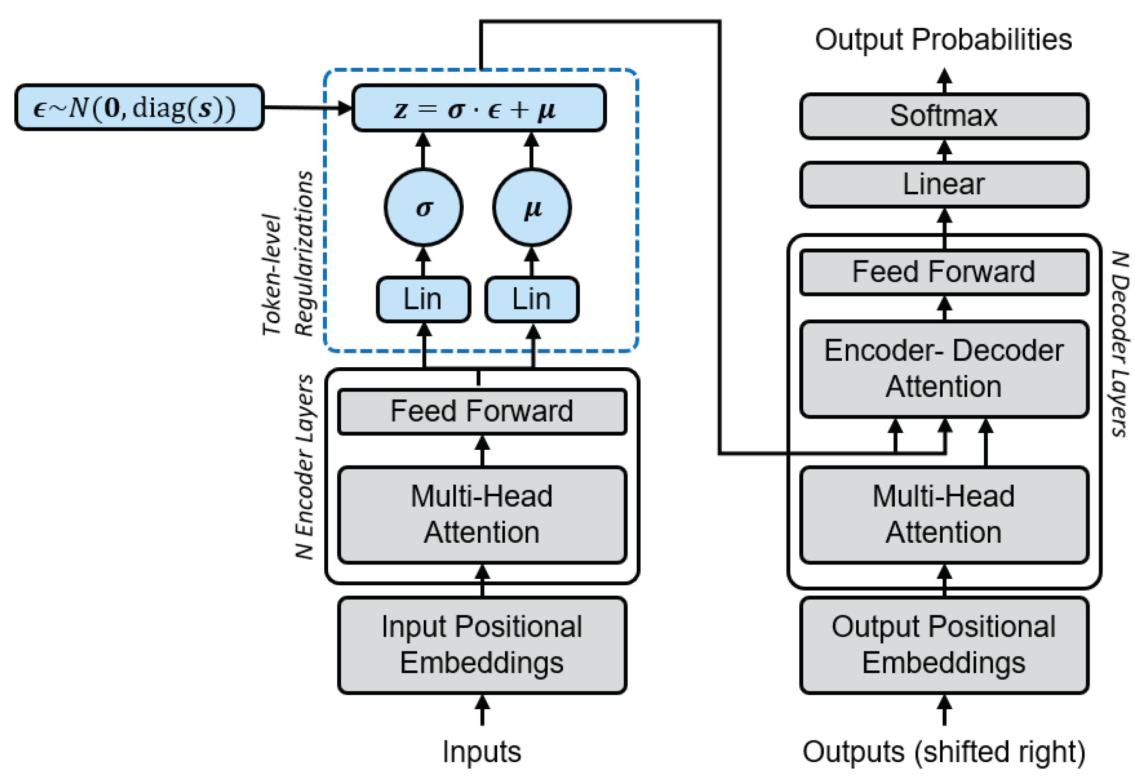
Initially proposed for machine translation, the Transformer [21] can be used as the language model and framed as an autoencoder. Extended with a token-level variational loss, the VAT maps input tokens to context-aware, distributed latent representations. Figure 1 illustrates the architecture of the VAT. The set of encoders E and decoders D is defined by the Transformer’s network architecture based on self-attention modules. The encoder maps the embedded input sequence , to a latent representation , , where T is the sequence length and d is the model dimension. In order to do so, the model predicts and from and samples . Z is then used as the attention source in the decoder to predict the next word based on the already produced output. As X and Z depend on T, the objective is to minimize
where and . More precisely, we let , where the vector is predicted, so that computing the actual value of involves the exponential as a nonlinear activation function.
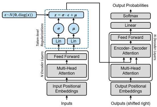
Figure 1.
The proposed Variational Auto-Transformer architecture: Mean and covariance for the variational loss (blue, dashed lines) are computed through two independent linear layers. The encoder and decoder (grey, solid lines) architecture is the same as in the original Transformer.
The output of the encoder is passed to two linear layers in parallel. The linear layers have the same number of input and output nodes and learn a transformation to predict and for each token. The latent representation Z is used as the input in the encoder-decoder attention layer of the Transformer’s decoder.
Scaling the Regularization Loss
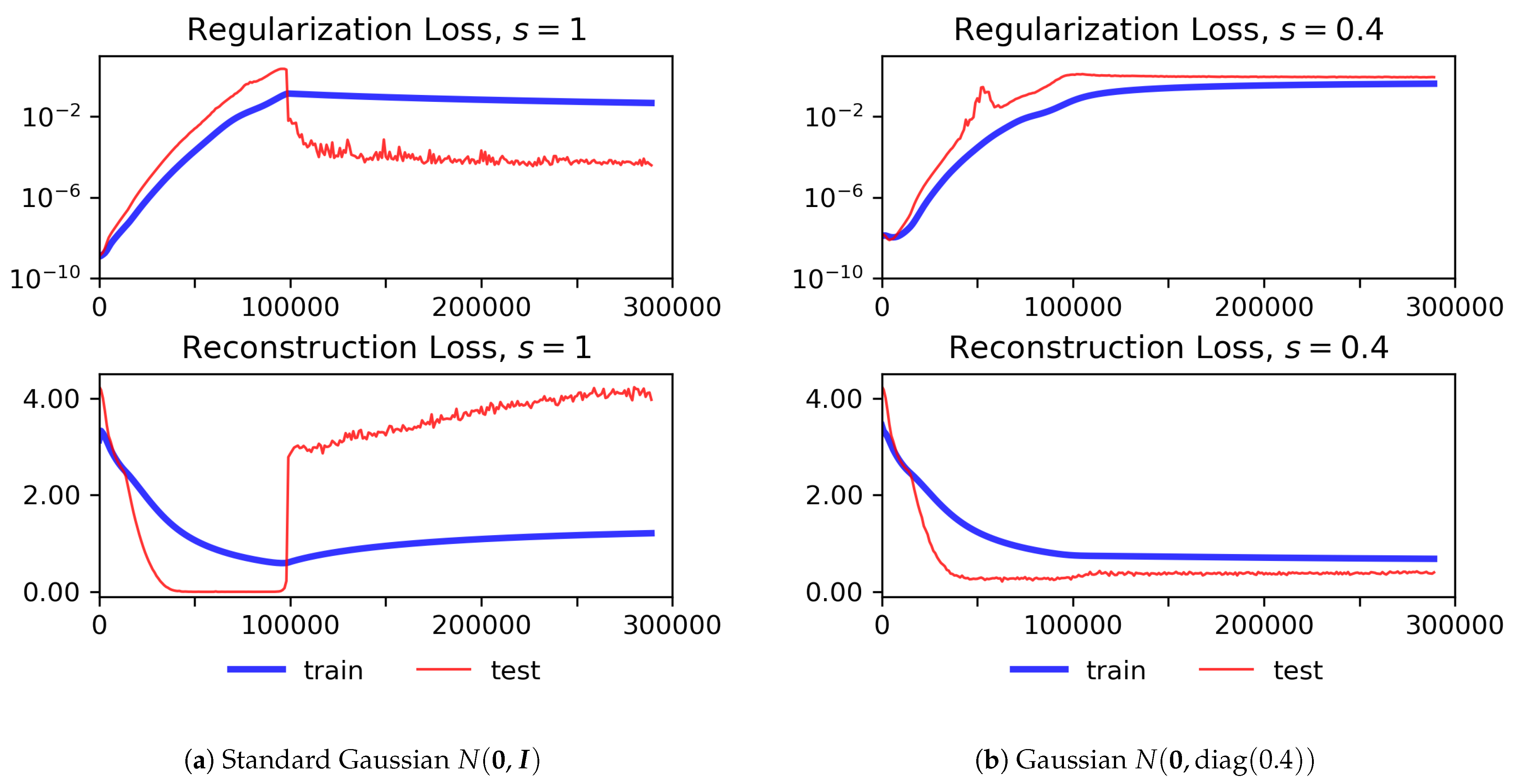
During our experiments, we experienced overfitting on the training data for the reconstruction loss. The learning curves of a corresponding experiment are illustrated in Figure 2a. Weighting the regularization loss according to a logistic annealing function as suggested by Bowman et al. [15] or by a scaling factor similar to the scaling of the beta-VAE [22], but with , only had a small effect.
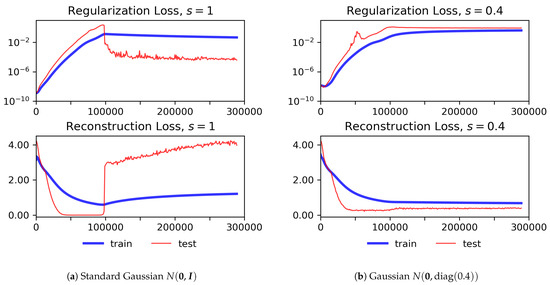
Figure 2.
Weighted regularization (top) and reconstruction loss (bottom) for training and test data over several epochs for two different Gaussians applied as a prior distribution for the regularization term.
Thus, we propose to scale the covariance matrix of the target distribution of instead. This is motivated by the observation that standard Gaussians in d-dimensional latent spaces (e.g., ) will overlap considerably if their mean values are—at the same time—regularized to zero. As a consequence, cannot be minimized by the model without increasing in an undesirable way. Scaling the standard deviation to a too small value, though, might result in peaky distributions, having no regulatory effect and resulting in a trivial reconstruction objective.
We adapted the computation of the regularization loss to incorporate a scaling factor s for the standard deviation as the hyperparameter. The closed-form of the VAE loss function (refer to Odaibo [23] for the derivation of the closed form) with a prior standard deviation and prior for a specific token’s layer outputs and becomes
This results in codes being distributed according to a Gaussian with zero mean and a predefined standard deviation, . The optimal balance between and as expressed by the value of is related to the representations’ isotropy and will be determined experimentally.
5. Experiments
The aim of the experiments is to balance the two loss terms. should be low to maintain the reconstruction ability of the network, while a too small scaling value s implies that the VAT essentially behaves as a regular AE, decoding from . At the same time, we want to optimize the isotropy of the latent representations. In order to choose the best setting, we observe both the resulting loss values and the properties of the latent space in terms of similarity between representations.
Our VAT model architecture is smaller than the original Transformer architecture, as it is not intended for machine translation, but autoencoding. The VAT model with dimensionality consists of encoder and decoder layers, respectively, with attention heads each. The dimension in the feed-forward layers is 512. Dropout during training was set to . The Noam optimizer [21] operates with 50,000 warmup steps. A logistic annealing function [15] with 50,000 warmup steps and an initial value of was applied to weight .
The VAT was trained on the training split of the WMT19 de-en dataset [24] using English sentences only. WMT19 contains data from news commentaries, Wiki titles, Europarl, ParaCrawl, and Common Crawl corpora. The data are tokenized using subword tokenization with a target vocabulary of tokens. The batch size was set to 128. Decoded sentences that are presented as results are obtained through beam search with beam size 5.
Optimal Scaling Parameter
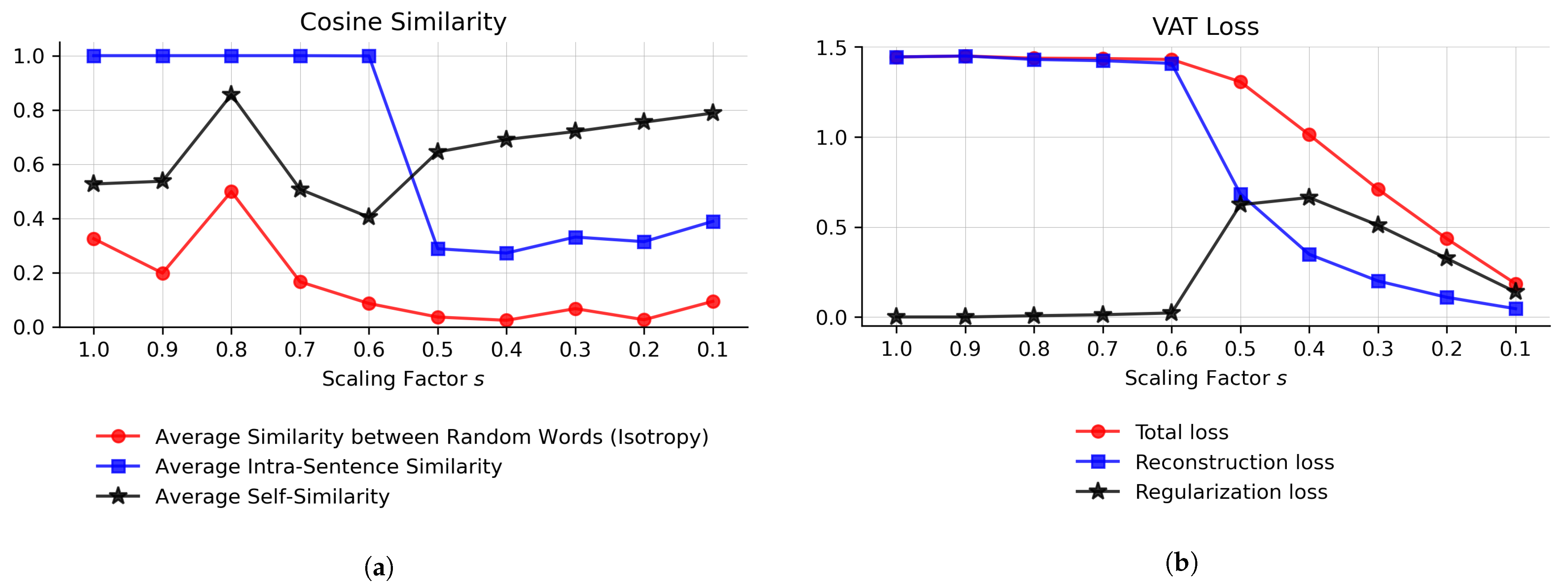
The isotropy of the learned representations is assessed as a function of the scaling factor . Ethayarajh [2] introduced the notion of isotropy of the latent space as the mean cosine similarity between vector representations of random tokens. In an isotropic latent space, representations of randomly sampled tokens have low cosine similarity and do not cluster in a specific direction.
In addition to isotropy, Ethayarajh [2] introduced the notion of self-similarity and intra-sentence similarity. A high self-similarity, i.e., mean cosine similarity between representations of the same token in different sentences, indicates that neighboring representations capture similar concepts, which contributes to the smoothness of the latent space. Intra-sentence similarity measures the mean cosine similarity of tokens occurring in the same sentence to the mean sentence representation, thus being related to contextuality.
BERT exhibits low isotropy (mean cosine similarity ) in its last layers [2], a phenomenon known as representation degeneration [3]. In contrast to BERT with high contextuality with respect to the low isotropy, we expect a more complete latent space for the VAT and, thus, high isotropy. The results in Figure 3a were computed for the STS12 datasets [25]. Different from Ethayarajh [2], Figure 3a depicts the plain intra-sentence and self-similarity, i.e., not adjusted for isotropy. The average cosine similarity between randomly sampled words is low for smaller s values, suggesting an isotropic latent space with representations distributed across space. The latent space is most isotropic at .

Figure 3.
Optimizing the scaling factor s with respect to isotropy and loss values. (a) Cosine similarities of the latent representations of the VAT at the end of the training process denoting the isotropy of the latent space and the contextuality of token representations; (b) reconstruction loss, weighted regularization loss, and total loss of the VAT at the end of the training process.
The average self-similarity of tokens greater than suggests a mapping of similar concepts into the same region, indicating smoothness in the latent space. The intra-sentence similarity for is lower than the self-similarity, but still above the similarity of random words. This indicates that contextual information is captured in the representations. Interestingly, for , the token representations seem to “collapse” into an identical representation for all positions in a sequence, resulting in an intra-sentence similarity of 1. Among the words with most context-specific representations are mainly stopwords, as they have the lowest self-similarity.
In Figure 3b, we report the final loss values after training the models for 3 epochs with different scaling factors . Scaling values result in near-zero regularization losses and high reconstruction error. The original input cannot be reproduced any more. This observation corresponds to the findings from Figure 3a, where the representations within a sentence are identical. Starting from , the reconstruction loss drops, and with , the reconstruction loss falls below the regularization loss. Values smaller than further decrease the positive effects of the variational model, as the achievable variety of generated text is reduced. This phenomenon is referred to as posterior collapse [26].
Combining the findings from evaluating the loss and latent space properties in Figure 3, we selected as the scaling factor for further evaluating the VAT. This value corresponds to good reconstruction ability and isotropic representations, which impacts both the generation of text, as well as the performance on classification tasks. Furthermore, the learning curves corresponding to no longer exhibit overfitting (see Figure 2b).
6. Variational Language Model
During training, the VAT encoder produces variants of the input tokens by drawing from the latent distribution. The VAT decoder has to be able to reproduce the original sequence given variational input. At test time, both approaches are possible: Decoding with the standard deviation set to 0, i.e., , leads to a deterministic representation and is used for classification tasks. For sequence generation, decoding allows generating variants of the original input sequence, a process we refer to as variational sampling. Variational language modeling thus denotes the various ways of manipulations and computations in the latent space that are possible with the VAT’s latent distributions. As examples, we discuss anecdotal results from variational sampling and interpolation.
Table 1 and Table 2 illustrate the generating capabilities of the VAT with variational sampling. In the second line in Table 1, the VAT is able to reconstruct the original sequence (first line), which refers to decoding with , i.e., without sampling. The following lines show exemplary variants of the input sentence obtained by randomizing the latent representations, displaying 12 variational samples. It is interesting that, while mostly maintaining the original sentence structure and original context, variants are found for almost all tokens. This gives an idea of the structure of the latent space and the contextuality of the representations. The approach is comparable to paraphrase generation, which is often obtained through back-translation [27,28] or by directly training on supervised data in the form of paraphrased sentence pairs [29].

Table 1.
Variational sampling. Example sentence (in bold) used as the input to the VAT, with the decoded mean representation and samples from the latent distribution (in italics).
Table 2.
Variational sampling. Example sentence in (bold) that was used as the input to the VAT, with only the underlined token being sampled. Samples from the latent distribution in italics.
Table 1 illustrates variational sampling for a single token, where the input sequence (in bold) is reconstructed according to , except for the underlined token, for which sampling is allowed. This setting is similar to a nearest neighbor search over a fixed corpus. The second line lists the obtained samples. By masking the underlined token, this approach is similar to gap filling [30,31]. Variational sampling, both for tokens and sequences, can be useful for generating paraphrases in tasks such as dialog generation or question answering.
We also experimented with latent space interpolation similar to [15,18,19]. We linearly interpolated the latent representations of two sentences (padded to the same length) with three intermediate steps. Decoding the intermediate representations results in the sentences illustrated in Table 3 for two examples. Observing a smooth interpolation trajectory as in the examples is not always the case. It is possible that after decoding, the intermediate steps are mapped to the same sentence, as seen for one sentence in the second example. This is especially true with the increasing size of the training data: the more training data, the more contextualized representations for the same word type that are mapped close to each other in latent space will exist.
Table 3.
Interpolation. First and last sentence (bold) were given as the input to the VAT. Intermediate sentences were obtained by tokenwise linear interpolation between the two latent representations padded to the same length.
For further investigations on the distribution of the variational samples and their distance from the mean representations, the distances between latent vectors in terms of their accumulated elementwise differences (i.e., over all dimensions and vectors in the representation of the sentence) were assessed. Figure 4 illustrates the histogram of these elementwise distances for the mean vectors of the start and end sentence from the second example in Table 3 in blue. For comparison, ten random sentences were drawn from the original start sentence (with the same approach as in Table 1). The red histogram shows the distribution of their elementwise differences. In order to illustrate the effect of the regularization term, experiments with different scaling values s are shown to determine the “signal-to-noise ratio”, where the differences between mean representations of start and end sentence are considered as the signal and those between the variational samples as noise. For , this ratio is on average. A closer, dimensionwise look at all vectors (not included in Figure 4) revealed that the peak value is 2 and is achieved in only one outlier dimension: even this “feature” is thus considerably affected by the variational random noise. The histograms for and are in line with the findings in Figure 3a,b, where the representations either collapse into an identical representation for the sentences () or the real distribution approximates the variational distribution more closely ().
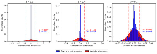
Figure 4.
Histogram of the elementwise difference between token vectors from the start and end sentence of the interpolation example in Table 3 (blue) and from the start sentence and 10 random variational samples of this sentence (red) for different scaling values s. denotes the value of the standard deviation of the corresponding distributions.
7. Sentence Representations
For the construction of sentence representations, we compared two pooling operations (average, sum). Additionally, the start token (“CLS”) representation was used as the embedding for the whole sentence, although this approach has been shown to be inferior to mean pooling in semantic similarity tasks for BERT [32]. We denote the different approaches as VAT-mean, VAT-sum, and VAT-start, respectively. We compared our model to the original BERT model (base) and, for a fair comparison in terms of model size, to a smaller variant with similar network dimensions as the VAT. BERT has encoder layers, and the model and representation dimension is . The smaller BERT model (https://github.com/google-research/bert, accessed on 8 June 2022) [33], which we refer to as MiniBERT, has and , the same size as the VAT. Both BERT and MiniBERT were trained on a much larger collection of datasets (Wikipedia, BookCorpus, CommonCrawl) than the VAT.
The sentence representations were tested using the SentEval [34] toolkit (https://github.com/facebookresearch/SentEval, accessed on 8 June 2022). The toolkit evaluates static sentence representations on two different classes of tasks: semantic similarity and sentence classification tasks. Table 4 lists the correlation values of the different sentence representation methods on the Semantic Textual Similarity (STS) tasks. For each pair of semantically similar sentences, the Spearman correlation rank between the cosine of their latent representations and a human-labeled gold standard (between 0 and 5) was computed (without fine-tuning or transfer learning). The correlation of VAT-based sentence representations is on par with BERT-based representations, which is surprising given the smaller model architecture and capacity of the VAT. For both VAT and BERT, start-token-based representations show less correlation than those obtained by average or sum pooling. Representations obtained from the MiniBERT model do not show any correlation at all, indicating that the BERT architecture requires a larger model size.
Table 4.
Spearman rank correlation between the cosine similarity of sentence representations and gold label similarity for different Semantic Textual Similarity (STS) tasks without fine-tuning the underlying models to the target data.
The classification tasks included in the SentEval toolkit comprise binary (MR, CR, SST2) and fine-grained (SST5) sentiment or polarity classification tasks, paraphrase detection (MRPC), natural language inference (SICK-E), and question-type classification (TREC) tasks. As paraphrase detection and natural language inference require the comparison of two sentences, the pair of input sentences was concatenated and separated by a special separation token to form a single-input vector. For the classification tasks, we compared the performance of the VAT to that of MiniBERT in two ways: in a feature-based approach and in a fine-tuning approach.
Both presented approaches are different from how state-of-the-art models are trained for transfer tasks. Given the smaller model capacity, we do not expect on-par performance, but rather want to better understand the kind of information stored in the representations and the potential that comes with additional classification layers on top of the model. The comparison to MiniBERT serves as the baseline.
For the feature-based approach, the sentence representations are extracted from the pre-trained models and then passed to a single classification layer trained with an Adam optimizer [35]. Given the results in Table 5 (top), the sum of the individual token representations is best suited as a standalone feature for sentence classification. As VAT-sum outperforms VAT-mean on all tasks, the dimensions of the latent representations seem to be well disentangled. With the exception of the SST2 task, the start representation yields the lowest accuracy values, suggesting that the first representations do not capture the full context of a sentence. MiniBERT, which is designed for fine-tuning rather than feature extraction, mostly does not reach the performance of the VAT variants. The difference between MiniBERT and VAT is especially large for the TREC task.
Table 5.
Dev/test accuracies on the SentEval transfer classification tasks. A single dense layer with nonlinear activation and the Adam optimizer is used as the classification layer. Bold values indicate the best test result for each task in the feature-based and fine-tuning approach.
For assessing the performance with a fine-tuning approach, we extended the underlying models by a single nonlinear dense classification layer and optimized with Adam. For the VAT, we only reused the encoder part to access the latent representations Z. For each task, we trained for five epochs and selected the best learning rate out of , , , and based on the validation set to be used on the test set. Note that the MiniBERT results can differ from the results in the original publication [33], as we did not further tune the model or the training process.
In Table 5 (bottom), we see a performance leap for all of the models compared to their feature-based results. While VAT-sum performed best for the feature-based approach, the method to produce sentence-level representations was not that decisive for the fine-tuning approach. The differences between sum, mean, and start were no longer as great as for the semantic similarity tasks, neither for MiniBERT nor for the VAT. It is interesting that MiniBERT is in the lead for sentiment classification tasks, whereas the VAT shows outstanding performance on the TREC (topic classification) task.
8. Discussion and Conclusions
The goal of the proposed VAT model is to obtain isotropic representations mapped to a smooth and complete latent space. The hyperparameter and scaling factor s is directly optimized to meet these criteria, thus reducing the effects of overfitting. The VAT is able to produce coherent sequences through manipulations directly in latent space. However, optimizing comes at the cost of . Perfect reconstruction of the original input is no longer possible at all times. However, this ability to produce variational samples will be especially useful in language generation tasks such as question answering. Conversational agents could benefit from paraphrases generated by variational sampling far as it would produce more nuanced and varied replies instead of deterministic answers.
Reducing the representations to a single sentence-level vector preserves contextual information. Semantic similarity tasks demonstrate that the smaller model capacity of the VAT is sufficient to capture semantic information that is on a par with larger BERT architectures. However, models explicitly trained to improve the performance on semantic similarity tasks are out of reach.
The VAT is able to produce more robust standalone sentence-level features when compared with MiniBERT for the feature-based classification approach. VAT outperforms the similar-sized MiniBERT also when being fine-tuned on sentence classification tasks, but is far from the state-of-the-art performance known from BERT-sized models with more sophisticated training procedures. Interestingly, the VAT shows its peak performance for the topic classification task TREC. In our setup, the VAT captures topic-related information even better than sentiment. A possible explanation could be that topic-related information is encoded in several token representations of a sentence. Sentiment might be inherent in less tokens and, thus, be underrepresented in the aggregated sentence representation.
Tasks involving the comparison of two sentences (MRPC, SICK-E), represented by a single concatenated vector, cannot be successfully solved by either the VAT or MiniBERT. Some model variants (MiniBERT included) only learn to predict the most frequent class. The reason could be the smaller model sizes, which are incapable of capturing the information of two concatenated sentences, as especially the VAT was never trained on such a setting. Instead of a concatenated vector, the comparison task could be solved using a Siamese network architecture, similar to Deudon et al. [10].
The comparison to MiniBERT leaves us optimistic that the results could be successfully extrapolated to larger models. We expect the performance on downstream tasks to improve while still maintaining the desired characteristics of the latent representations supporting semantic reasoning through vector space arithmetic. The optimization of the regularization loss at the token level could even allow the training of a multilingual model or a translation model, given sufficient training data.
Author Contributions
Conceptualization, C.F. and S.W.; methodology, C.F. and S.W.; software, C.F.; validation, C.F.; formal analysis, C.F. and S.W.; investigation, C.F.; data curation, C.F.; writing–original draft preparation, C.F.; writing–review and editing, C.F. and S.W.; visualization, C.F.; supervision, C.F. and S.W.; project administration, C.F. and S.W.; funding acquisition, S.W. All authors have read and agreed to the published version of the manuscript.
Funding
This project is partially funded by the Science and Innovation Strategy Salzburg (WISS 2025) project “IDA-Lab Salzburg”, Grant Number 20102-F1901166-KZP.
Data Availability Statement
The data used in this study are openly available: WMT19 [24] is available through the tensorflow library at https://www.tensorflow.org/datasets/catalog/wmt19_translate (accessed on 8 June 2022). SentEval [34] is available from Facebook Research at https://github.com/facebookresearch/SentEval (accessed on 8 June 2022).
Acknowledgments
The authors want to thank Salzburg University of Applied Sciences for its doctoral support program, which facilitated the work on the publication.
Conflicts of Interest
The authors declare no conflict of interest.
References
- Devlin, J.; Chang, M.W.; Lee, K.; Toutanova, K. BERT: Pre-training of Deep Bidirectional Transformers for Language Understanding. In Proceedings of the 2019 Conference of the North American Chapter of the Association for Computational Linguistics: Human Language Technologies, Volume 1 (Long and Short Papers), Minneapolis, MN, USA, 2–7 June 2019; pp. 4171–4186. [Google Scholar]
- Ethayarajh, K. How Contextual are Contextualized Word Representations? Comparing the Geometry of BERT, ELMo, and GPT-2 Embeddings. In Proceedings of the 2019 Conference on Empirical Methods in Natural Language Processing and the 9th International Joint Conference on Natural Language Processing (EMNLP-IJCNLP), Hong Kong, China, 3–7 November 2019; pp. 55–65. [Google Scholar]
- Gao, J.; He, D.; Tan, X.; Qin, T.; Wang, L.; Liu, T. Representation Degeneration Problem in Training Natural Language Generation Models. In Proceedings of the International Conference on Learning Representations, New Orleans, LA, USA, 6–9 May 2019. [Google Scholar]
- Wang, L.; Huang, J.; Huang, K.; Hu, Z.; Wang, G.; Gu, Q. Improving Neural Language Generation with Spectrum Control. In Proceedings of the International Conference on Learning Representations, Addis Ababa, Ethiopia, 26–30 April 2020. [Google Scholar]
- Li, B.; Zhou, H.; He, J.; Wang, M.; Yang, Y.; Li, L. On the Sentence Embeddings from Pre-trained Language Models. In Proceedings of the 2020 Conference on Empirical Methods in Natural Language Processing (EMNLP), Online, 16–20 November 2020; pp. 9119–9130. [Google Scholar]
- Kingma, D.P.; Welling, M. Auto-Encoding Variational Bayes. In Proceedings of the International Conference on Learning Representations, Banff, AB, Canada, 14–16 April 2014. [Google Scholar]
- Goodfellow, I.; Bengio, Y.; Courville, A. Deep Learning; MIT Press: Cambridge, MA, USA, 2016. [Google Scholar]
- Gururangan, S.; Dang, T.; Card, D.; Smith, N.A. Variational Pretraining for Semi-supervised Text Classification. In Proceedings of the 57th Annual Meeting of the Association for Computational Linguistics, Florence, Italy, 28 July–2 August 2019; pp. 5880–5894. [Google Scholar]
- Mahabadi, R.K.; Belinkov, Y.; Henderson, J. Variational Information Bottleneck for Effective Low-Resource Fine-Tuning. In Proceedings of the International Conference on Learning Representations, Virtual, 3–7 May 2021. [Google Scholar]
- Deudon, M. Learning Semantic Similarity in a Continuous Space. In Advances in Neural Information Processing Systems; Bengio, S., Wallach, H., Larochelle, H., Grauman, K., Cesa-Bianchi, N., Garnett, R., Eds.; Curran Associates, Inc.: New York, NY, USA, 2018; Volume 31. [Google Scholar]
- Zhao, T.; Lee, K.; Eskenazi, M. Unsupervised Discrete Sentence Representation Learning for Interpretable Neural Dialog Generation. In Proceedings of the 56th Annual Meeting of the Association for Computational Linguistics, Melbourne, Australia, 15–20 July 2018; pp. 1098–1107. [Google Scholar]
- Miao, Y.; Yu, L.; Blunsom, P. Neural Variational Inference for Text Processing. In Proceedings of the 33rd International Conference on Machine Learning (ICML’16), New York, NY, USA, 20–22 June 2016; Volume 48, pp. 1727–1736. [Google Scholar]
- Wang, T.; Wan, X. T-CVAE: Transformer-Based Conditioned Variational Autoencoder for Story Completion. In Proceedings of the IJCAI, Macao, China, 10–16 August 2019; pp. 5233–5239. [Google Scholar]
- Shu, R.; Lee, J.; Nakayama, H.; Cho, K. Latent-variable Non-autoregressive Neural Machine Translation with Deterministic Inference using a Delta Posterior. In Proceedings of the AAAI Conference on Artificial Intelligence, New York, NY, USA, 7–12 February 2020; Volume 34, pp. 8846–8853. [Google Scholar]
- Bowman, S.R.; Vilnis, L.; Vinyals, O.; Dai, A.; Jozefowicz, R.; Bengio, S. Generating Sentences from a Continuous Space. In Proceedings of the 20th SIGNLL Conference on Computational Natural Language Learning, Berlin, Germany, 11–12 August 2016; pp. 10–21. [Google Scholar]
- Fang, L.; Li, C.; Gao, J.; Dong, W.; Chen, C. Implicit Deep Latent Variable Models for Text Generation. In Proceedings of the 2019 Conference on Empirical Methods in Natural Language Processing and the 9th International Joint Conference on Natural Language Processing (EMNLP-IJCNLP), Hong Kong, China, 3–7 November 2019; pp. 3946–3956. [Google Scholar]
- Yang, Z.; Hu, Z.; Salakhutdinov, R.; Berg-Kirkpatrick, T. Improved Variational Autoencoders for Text Modeling Using Dilated Convolutions. In Proceedings of the 34th International Conference on Machine Learning (ICML’17), Sydney, NSW, Australia, 6–11 August 2017; Volume 70, pp. 3881–3890. [Google Scholar]
- Liu, D.; Liu, G. A Transformer-Based Variational Autoencoder for Sentence Generation. In Proceedings of the International Joint Conference on Neural Networks (IJCNN), Budapest, Hungary, 14–19 July 2019; pp. 1–7. [Google Scholar]
- Li, C.; Gao, X.; Li, Y.; Peng, B.; Li, X.; Zhang, Y.; Gao, J. Optimus: Organizing Sentences via Pre-trained Modeling of a Latent Space. In Proceedings of the 2020 Conference on Empirical Methods in Natural Language Processing (EMNLP), Virtual, 16–20 November 2020; pp. 4678–4699. [Google Scholar]
- Li, R.; Li, X.; Chen, G.; Lin, C. Improving Variational Autoencoder for Text Modelling with Timestep-Wise Regularisation. In Proceedings of the 28th International Conference on Computational Linguistics, Online, 8–13 December 2020; pp. 2381–2397. [Google Scholar]
- Vaswani, A.; Shazeer, N.; Parmar, N.; Uszkoreit, J.; Jones, L.; Gomez, A.N.; Kaiser, Ł; Polosukhin, I. Attention is All you Need. In Advances in Neural Information Processing Systems 30; Curran Associates, Inc.: New York, NY, USA, 2017; pp. 5998–6008. [Google Scholar]
- Higgins, I.; Matthey, L.; Pal, A.; Burgess, C.; Glorot, X.; Botvinick, M.; Mohamed, S.; Lerchner, A. beta-VAE: Learning Basic Visual Concepts with a Constrained Variational Framework. In Proceedings of the International Conference on Learning Representations, Toulon, France, 24–26 April 2017. [Google Scholar]
- Odaibo, S. Tutorial: Deriving the Standard Variational Autoencoder (VAE) Loss Function. arXiv 2019. Available online: arxiv:1907.08956.
- Barrault, L.; Bojar, O.; Costa-Jussà, M.; Federmann, C.; Fishel, M.; Graham, Y.; Haddow, B.; Huck, M.; Koehn, P.; Malmasi, S.; et al. Findings of the 2019 Conference on Machine Translation (WMT19). In Proceedings of the Fourth Conference on Machine Translation (Volume 2: Shared Task Papers, Day 1), Florence, Italy, 1–2 August 2019; pp. 1–61. [Google Scholar]
- Agirre, E.; Cer, D.; Diab, M.; Gonzalez-Agirre, A. SemEval-2012 Task 6: A Pilot on Semantic Textual Similarity. *SEM 2012: The First Joint Conference on Lexical and Computational Semantics—Volume 2. In Proceedings of the Sixth International Workshop on Semantic Evaluation (SemEval 2012), Montréal, QC, Canada, 7–8 June 2012; pp. 385–393. [Google Scholar]
- Lucas, J.; Tucker, G.; Grosse, R.; Norouzi, M. Understanding Posterior Collapse in Generative Latent Variable Models. In Proceedings of the International Conference on Learning Representations, DeepGenStruct Workshop, New Orleans, LA, USA, 6–9 May 2019. [Google Scholar]
- Sennrich, R.; Haddow, B.; Birch, A. Improving Neural Machine Translation Models with Monolingual Data. In Proceedings of the 54th Annual Meeting of the Association for Computational Linguistics, Berlin, Germany, 7–12 August 2016; pp. 86–96. [Google Scholar]
- Wieting, J.; Gimpel, K. ParaNMT-50M: Pushing the Limits of Paraphrastic Sentence Embeddings with Millions of Machine Translations. In Proceedings of the 56th Annual Meeting of the Association for Computational LinguisticsMelbourne, Australia, 15–20 July 2018; pp. 451–462. [Google Scholar]
- Gupta, A.; Agarwal, A.; Singh, P.; Rai, P. A deep generative framework for paraphrase generation. In Proceedings of the AAAI Conference on Artificial Intelligence, New Orleans, LA, USA, 2–7 February 2018; Volume 32. [Google Scholar]
- Donahue, C.; Lee, M.; Liang, P. Enabling Language Models to Fill in the Blanks. In Proceedings of the 58th Annual Meeting of the Association for Computational Linguistics, Online, 5–10 July 2020; pp. 2492–2501. [Google Scholar]
- Wu, X.; Zhang, T.; Zang, L.; Han, J.; Hu, S. Mask and Infill: Applying Masked Language Model for Sentiment Transfer. In Proceedings of the Twenty-Eighth International Joint Conference on Artificial Intelligence, IJCAI-19, International Joint Conferences on Artificial Intelligence Organization, Vienna, Austria, Macao, China, 10–16 August 2019; pp. 5271–5277. [Google Scholar]
- Reimers, N.; Gurevych, I. Sentence-BERT: Sentence Embeddings using Siamese BERT-Networks. In Proceedings of the 2019 Conference on Empirical Methods in Natural Language Processing and the 9th International Joint Conference on Natural Language Processing (EMNLP-IJCNLP), Hong Kong, China, 3–7 November 2019; pp. 3982–3992. [Google Scholar]
- Turc, I.; Chang, M.W.; Lee, K.; Toutanova, K. Well-Read Students Learn Better: On the Importance of Pre-training Compact Models. arXiv 2019. Available online: arxiv:1908.08962v2.
- Conneau, A.; Kiela, D. SentEval: An Evaluation Toolkit for Universal Sentence Representations. In Proceedings of the Eleventh International Conference on Language Resources and Evaluation (LREC 2018); European Language Resources Association (ELRA), Miyazaki, Japan, 7–12 May 2018. [Google Scholar]
- Kingma, D.P.; Ba, J. Adam: A Method for Stochastic Optimization. In Proceedings of the International Conference on Learning Representations, San Diego, CA, USA, 7–9 May 2015. [Google Scholar]

Publisher’s Note: MDPI stays neutral with regard to jurisdictional claims in published maps and institutional affiliations. |
© 2022 by the authors. Licensee MDPI, Basel, Switzerland. This article is an open access article distributed under the terms and conditions of the Creative Commons Attribution (CC BY) license (https://creativecommons.org/licenses/by/4.0/).