3.2. Basics of One-Class Classification Quality and Adversarial Samples
Consider the problem of synthesizing a classifier using the machine learning method. For simplicity, we take the problem of one-class classification. Denote by
the set of classified objects. For a one-class classifier, the output is
, with 1 indicating membership in the target class and 0 indicating no membership. The subset corresponding to the target class will be denoted as
. Allow the object membership function to be set to the target class:
This function is an ideal one-class classifier, however, in practice, as a rule, it is not possible to obtain all
values and use them for training. Usually, a limited countable training set
is available, from which a training sample is formed, as well as samples to control the training and testing process. Denote the trained one-class classifier:
Despite the fact that
is trained on
, as a result of the synthesis, various situations are possible that correspond to the possible outcomes of the binary classification (
Table 2): True Positive (
), True Negative (
), False Positive (
), False Negative (
).
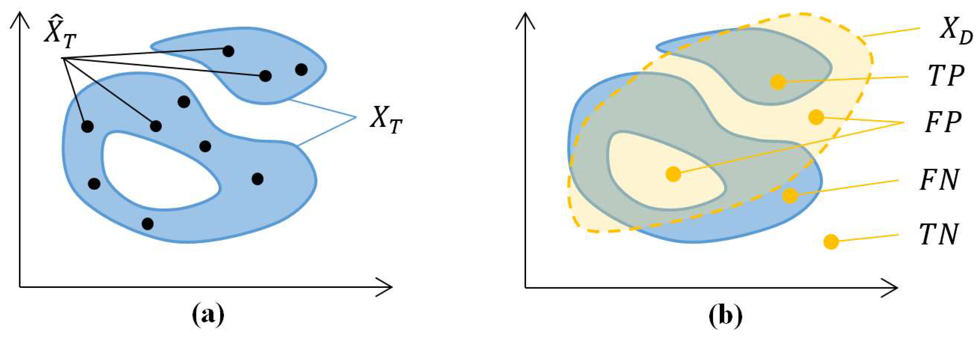
In fact, the real one-class classifier differs from the ideal one in that the set of objects that it refers to the target class is deformed, that is, it differs from the target
:
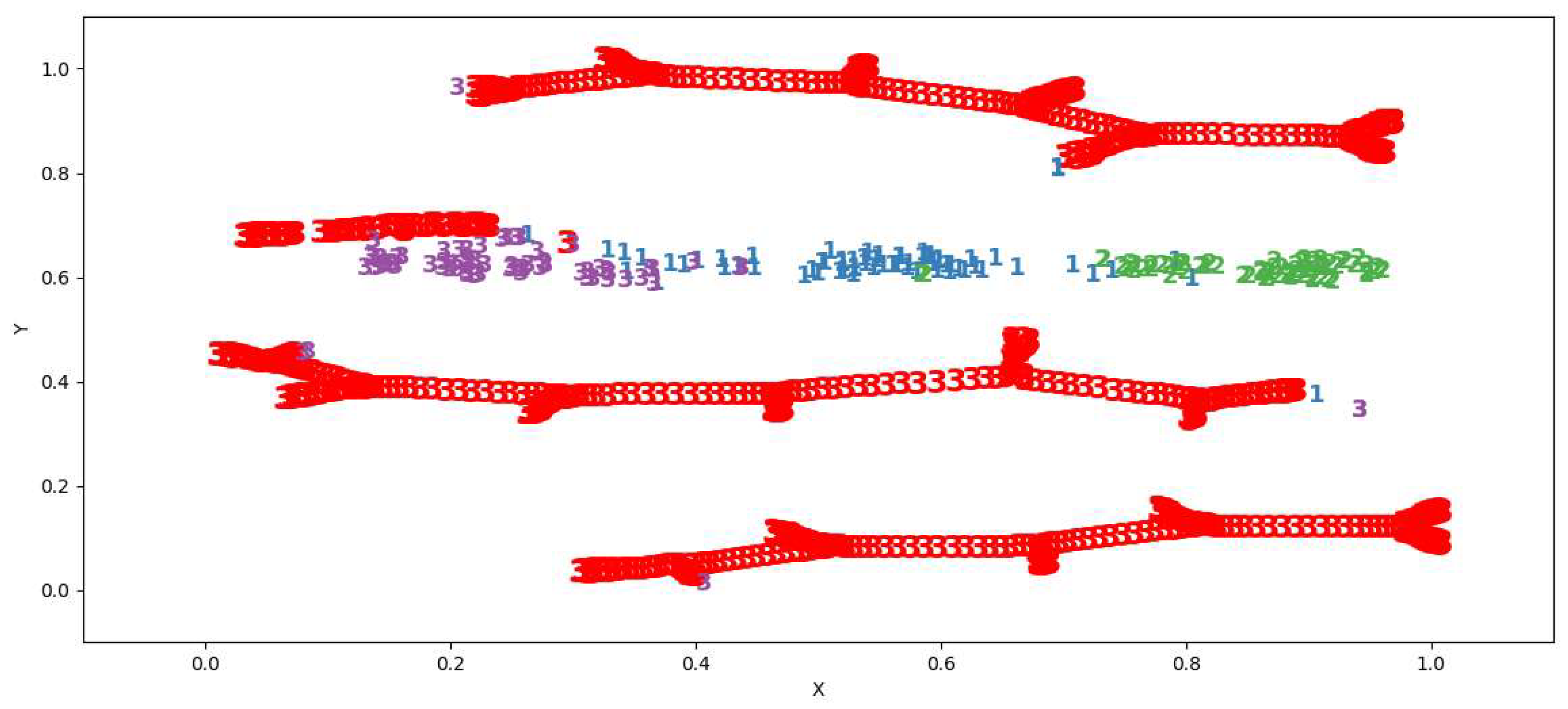
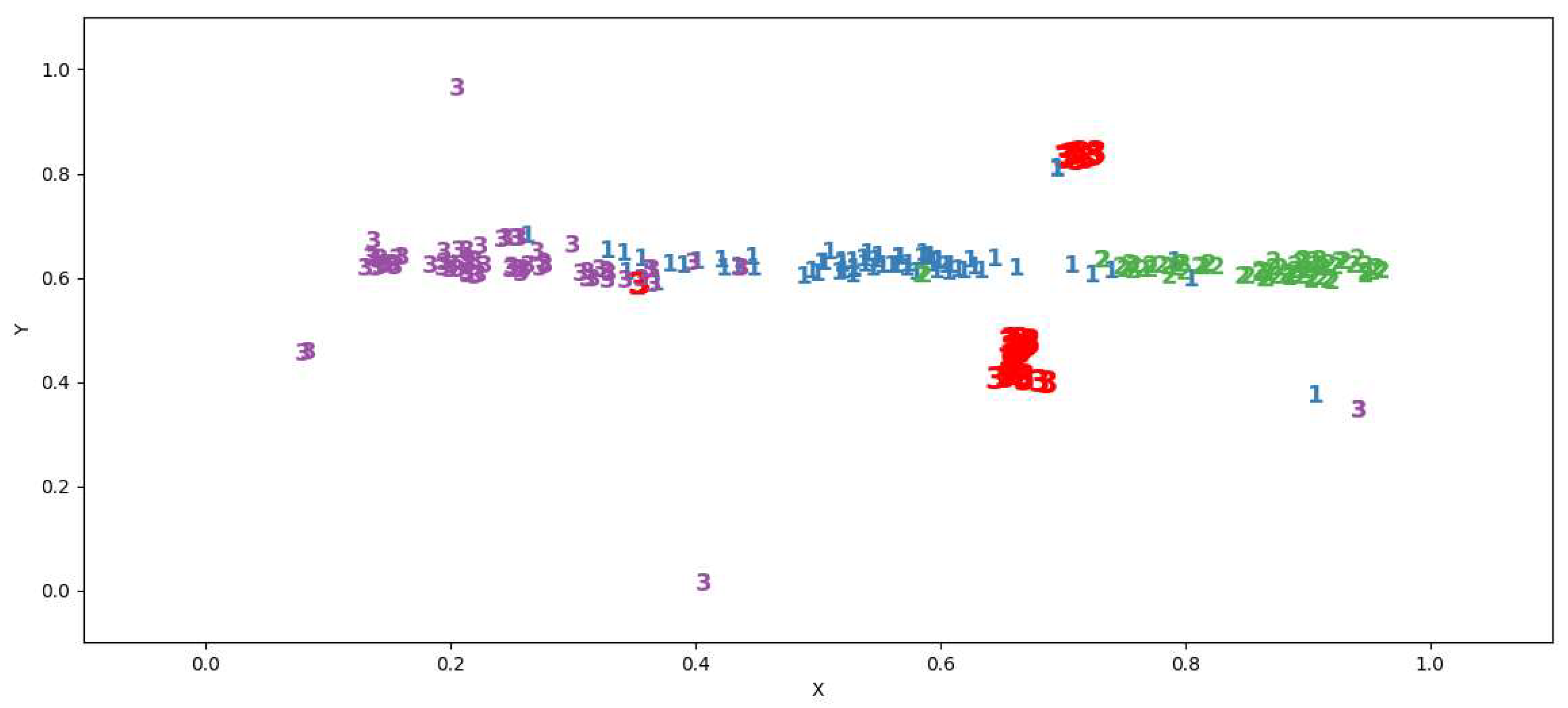
A similar situation can be visualized in
Figure 2.
The quality of a one-class classifier is the closeness of
to the ideal
, which can be expressed in terms of the properties of the
set compared to the
set. In particular, the classification outcomes
and
differ from the ideal. Situation FP corresponds to the case
, and situation
corresponds to the case
, where the operation\denotes the subtraction of sets. For continuous sets of classification points, we can introduce the concept of volume, for which we use the notation
, and
. In this case, the presence of situations
and
can be described in terms of volume as follows:
Note that the adversarial examples for a one-class classifier form the set
. The outcome of a correct classification is described in terms of volume:
Moreover, follows from .
It is desirable that the numerical assessment of the quality of the classifier does not depend on the volume of the target set, which will make it possible to compare the quality of classifiers trained for various applied problems. Let us introduce quality indicators normalized to the volume of the target set:
The quality indicator takes on a value greater than 0 if incorrectly classifies objects outside the target set. The quality indicator takes a value from 0 to 1, and if incorrectly classifies objects within the target set, then the metric is greater than 0. The limit value is the situation when the target and classified sets do not intersect. The quality indicator takes values from 0 to 1, and the value 0 corresponds to the zero intersection of the sets and , which is difficult to imagine with any effective machine learning procedure, and 1 corresponds to the usual situation when the classifier makes the right decision on the entire area of training data.
The target set approximation accuracy can be estimated as the ratio of the volume of the target set to the volume deformed by the classifier:
An ideal one-class classifier is characterized by the following values of quality indicators:
Taken together, the proposed quality indicators form a multidimensional criterion, which for brevity we will denote as EDCA. This criterion was introduced by the authors in [
36] in order to numerically evaluate the quality of an anomaly detector based on a neural network auto-encoder.
In reality, the set of points in the training dataset is discrete. In order to be able to calculate the proposed quality indicators for real classifiers, it is necessary to introduce a grid approximation of a continuous space with the restriction of a certain work area in which we will calculate the quality indicators. By limiting the space to a workspace that obviously includes sets of training and test data, we can normalize the coordinates in the range from 0 to 1. Let us introduce a uniform grid with step h over all coordinates of the limited grid space. Thus, for an -dimensional feature space, we will have grid space cells. Let us call the set of these cells the scan set . We will attribute the points of the sets and to the cells of the scan set to which they belong. Thus, the cells of the training data form the set , and the set will be formed from cells with a positive classification result for the point in the center of the cell.
It is recommended to choose the cell size for the data set under study so that the number of training set points in each cell is balanced and tends to 1. If the cell size is too small, then in the case of high data dimension, the calculations will require significantly more time. In addition, a too small value of will lead to the fact that neighboring points will be separated in the scan set by several empty cells that do not belong to , which can lead to the loss of significance of the EDCA numerical estimates.
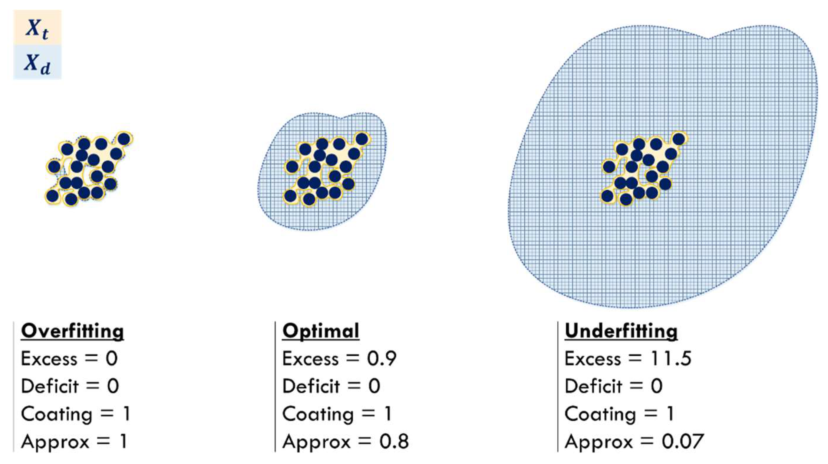
An example of EDCA numerical estimates for a single-class classifier is shown in
Figure 3.
Values , largely characterize the quality of classification in the classical sense.
The
characteristic is the most important for assessing the vulnerability of a classifier to adversarial attacks. This characteristic shows the size of the area of positive classification in the feature space outside the boundaries of the area of training examples.
Figure 3 shows that the larger this area, the larger the value of
. Comparing the
characteristics of different classifiers allows one to compare the risk of adversarial attacks, quantified by the amount of feature space in which examples that cause classifier errors can be found. It should be noted that the calculation of
is performed without knowledge of the classifier mechanisms (black-box) and can be used to compare classifiers of different nature.
The characteristic shows how closely the area of positive classification matches the training set. In case the classifier is too promiscuous and prone to adversarial attacks, the value is close to 0.
It should be noted that the “ideal” classifier, characterized by the limiting values of the characteristics, is vulnerable to the FN classification errors in the case of a non-representative training sample. Classification errors like this can also be considered adversarial attacks in some way.
If, due to the specifics of the problem being solved, FP errors are more critical than errors of the second kind, then it is recommended to choose a classifier that provides the minimum value.
3.3. Principles of the Proposed Criteria for Assessing Quality of Multiclass Classifiers
As noted earlier, classical classification quality estimates based on an error matrix cannot fully characterize the properties of a classifier synthesized by machine learning methods. To solve the problem of assessing the resistance of a classifier to adversarial attacks, it is proposed to analyze the behavior of the trained classifier in the area of the feature space in the vicinity of the training set. Consider the estimation method on the example of a classifier trained on the training data set . Let us say the training set includes classes. Let us denote the set of examples from the training set corresponding to class as , where . The set of samples that the trained classifier recognizes as class will be denoted as .
For a numerical evaluation of the properties of a multiclass classifier, a multidimensional EDCA criterion can be used, which includes the previously introduced characteristics for each of the classes. In this case, for each of the classes, their own characteristics
,
,
,
can be calculated. This criterion was first used to assess the quality of a classifier developed for dynamic classification under concept drift [
37] and was also studied for comparison with classical quality estimates based on an error matrix [
38].
For the case of multiclass classification, a characteristic feature is also the partial overlap of areas containing examples belonging to different classes. For example, the Iris data set [
13] has such a feature. In this case, the construction of an ideal classifier seems impossible in principle, which is well known to machine learning researchers.
A characteristic of the ambiguity of the training data set is a non-zero intersection of the regions of classes
and
:
In the domain of ambiguous classifier definition, any example will be adversarial in some sense. A reasonable characteristic for evaluating the behavior of a multiclass classifier in the area of ambiguity can be an assessment of its preference
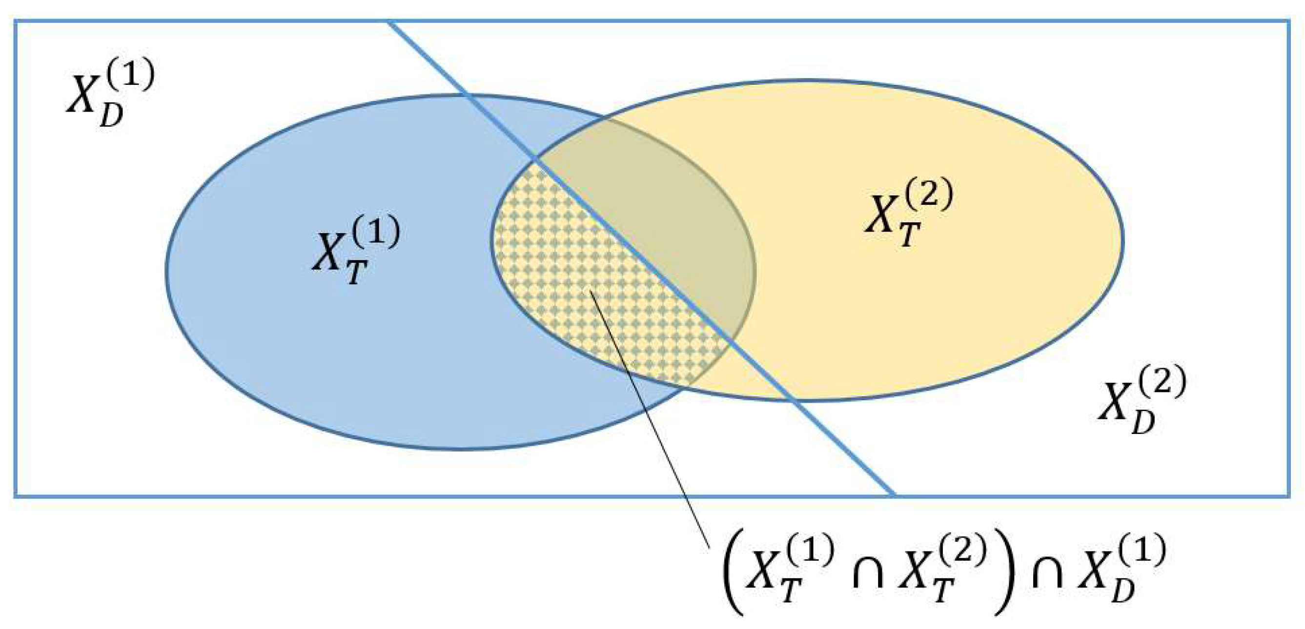
for one class over all the others. For the intersection of two classes, such a characteristic can be calculated as the ratio of the volume of the domain of belonging to a particular class to the volume of the domain of ambiguous definition:
Graphically, the preference area is shown in
Figure 4.
Generalizing the definition for the case of intersections of the domains of definition of several classes, we get:
The value of changes from 0 to 1 and shows how the classifier in areas of ambiguity tends to make a decision in favor of class . For practical application, this characteristic should be calculated for the cells of the scan set.
Thus, to numerically characterize the properties of a multiclass classifier, it is proposed to calculate for each of the classes , , , , .
The use of a quality criterion, the size of which depends on the number of classes, seems inconvenient. At the same time, if we do not have preferences for the significance of a particular class, then a tuple of 5 values of
,
,
,
,
can be considered a reasonable numerical assessment of the quality of the classifier, each of which characterizes the classifier in the worst way for all classes:
For the characteristics , , and , the worst value (minimum or maximum) is taken, and for —the sum of all classes. The set of proposed characteristics form a multidimensional EDCAP quality criterion, which can be used to compare classifiers, taking into account the possible intersection of the definition areas of some classes. The calculation of EDCAP characteristics must be carried out on the same scan set, that is, with the same working area and grid spacing.
Let an adversarial attack on class be an example that is different from the examples belonging to class , but classified as belonging to it. Then, to assess the vulnerability of the classifier to adversarial attacks on class , the most valuable characteristic is , however, in cases of overlapping areas, it is also necessary to analyze .
In this case, the task of comparing two classifiers in terms of their vulnerability to adversarial attacks can be reduced to comparing the calculated values in the case of non-overlapping training sets. A classifier with a lower value has a smaller area containing adversarial samples for all classes.
3.4. Principles of the Proposed Method of Synthesis for Adversarial Attack-Resistant Classifiers
Consider the problem of designing a classifier resistant to adversarial attacks. To assess stability, we will use the EDCAP criterion. First, it is necessary to analyze the properties of traditional classifiers obtained as a result of machine learning. To do this, it is convenient to use the approach used to calculate the EDCAP quality indicators with visualization of the
and
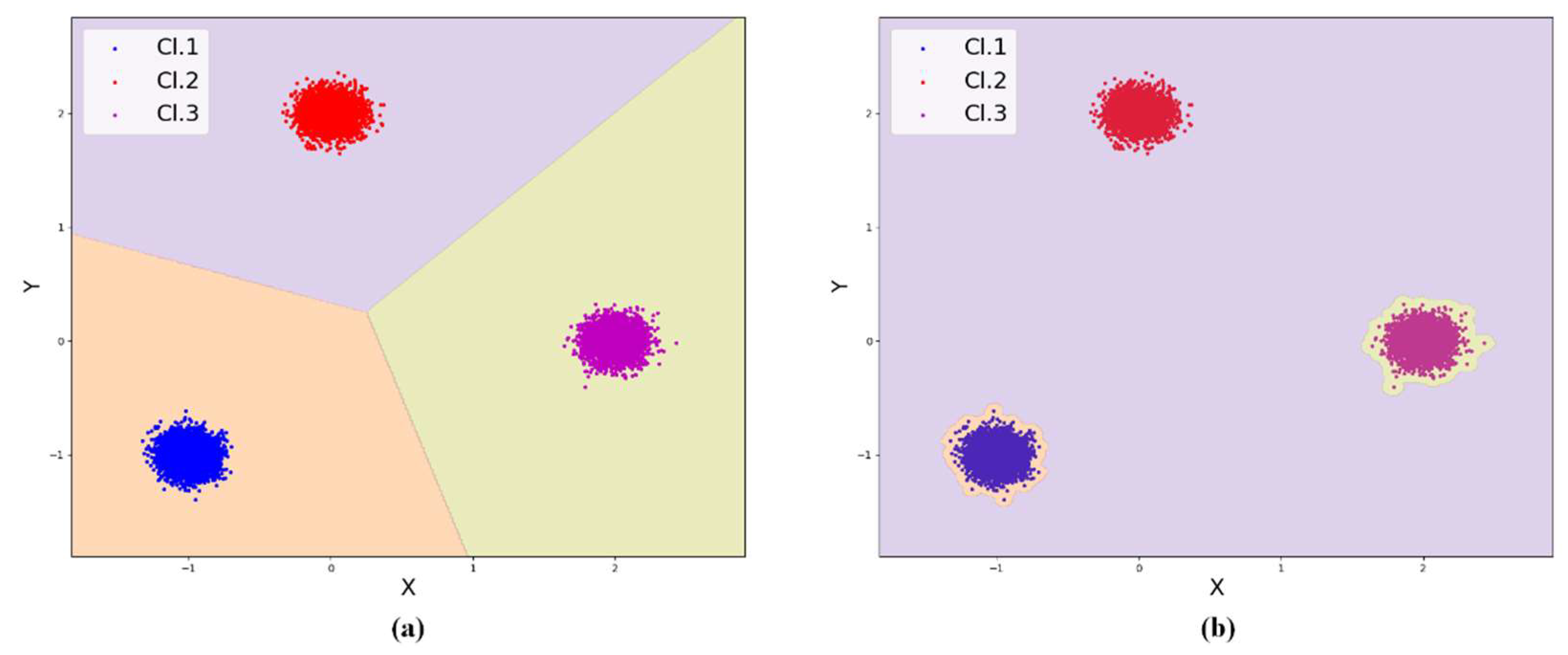
areas for all classes. Typical cases are shown in
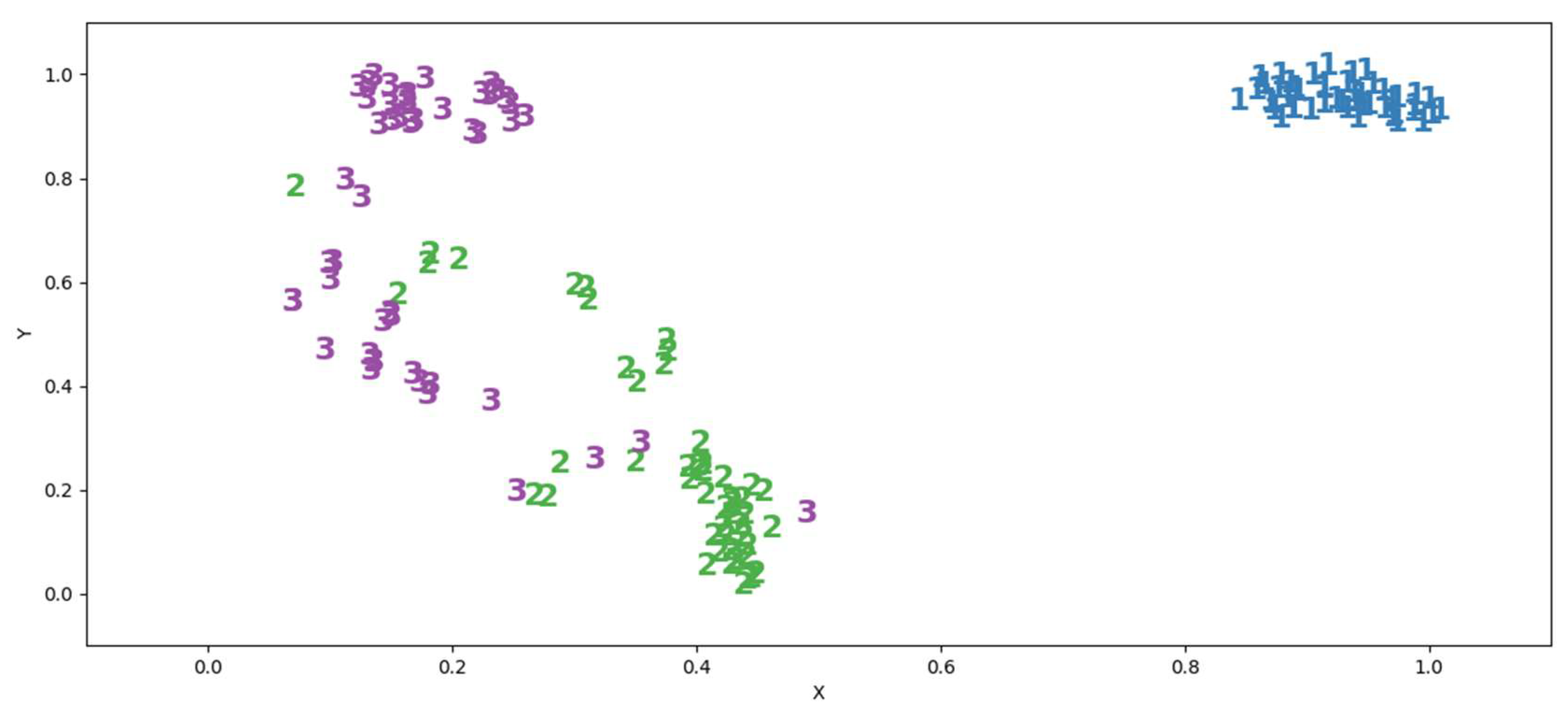
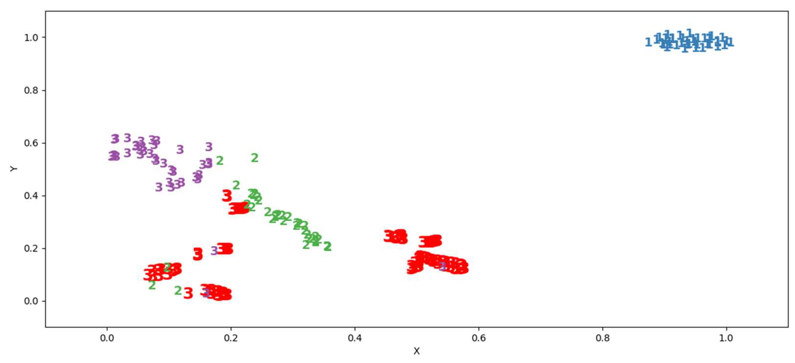
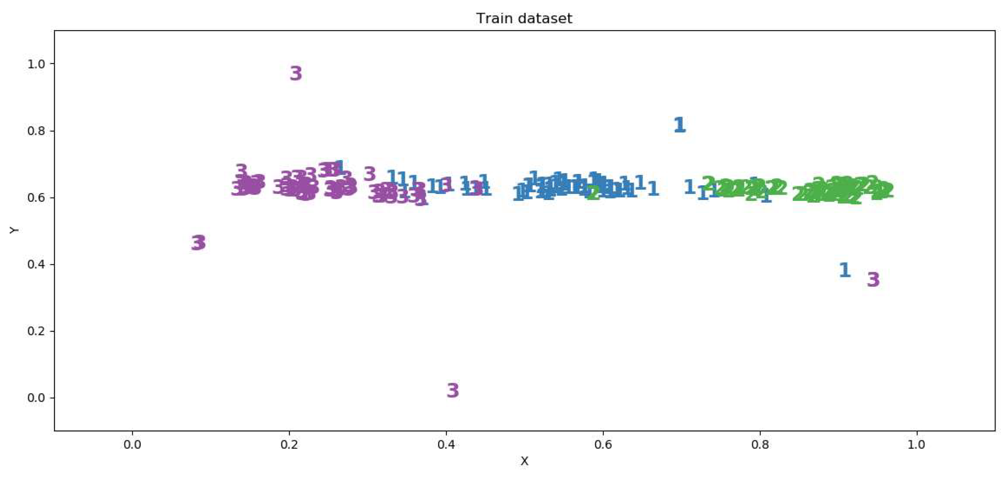
Figure 5.
Such options for splitting the feature space after training are the cause of classifier errors. For example, in case
Figure 5a any example, even far enough away from the scope of the class given by the training set, will be classified as belonging to this class. The use of such a classifier is undesirable for a number of practical tasks, for example, in intrusion detection systems. In case
Figure 5b, examples close to the scope of classes Cl.1 and Cl.3 will be classified as belonging to class Cl.2. On the classifier in case
Figure 5b, it is possible to generate a set of adversarial examples that cause false positive errors for classes Cl.1 and Cl.3, and a set of adversarial examples that cause false negative errors for class Cl.2. The use of such a classifier in computer vision and autopilot systems can lead to serious consequences due to the wrong decision.
The described situations can be avoided if an ensemble of auto-encoders is used for classification. Each ensemble auto-encoder in the learning process seeks to build a compact region that spans many training examples of the target class. Let us construct a multiclass classification algorithm based on an ensemble of auto-encoders. Each of the auto-encoders should be trained only on examples of one of the classes. Examples from other classes for this auto-encoder are anomalies. The main property of the auto-encoder is a small reconstruction error for examples from the training set and those close to them. A large reconstruction error indicates that similar examples did not appear in the learning process. To separate familiar examples from unfamiliar examples, the reconstruction error threshold is used, which determines the sensitivity of the algorithm to novelty.
In addition to class-specific auto-encoders, it is useful to introduce an auto-encoder that will separate examples of known classes from examples that are unlike any of the classes. Such an auto-encoder acts as an anomaly detector and is an additional defense against adversarial attacks.
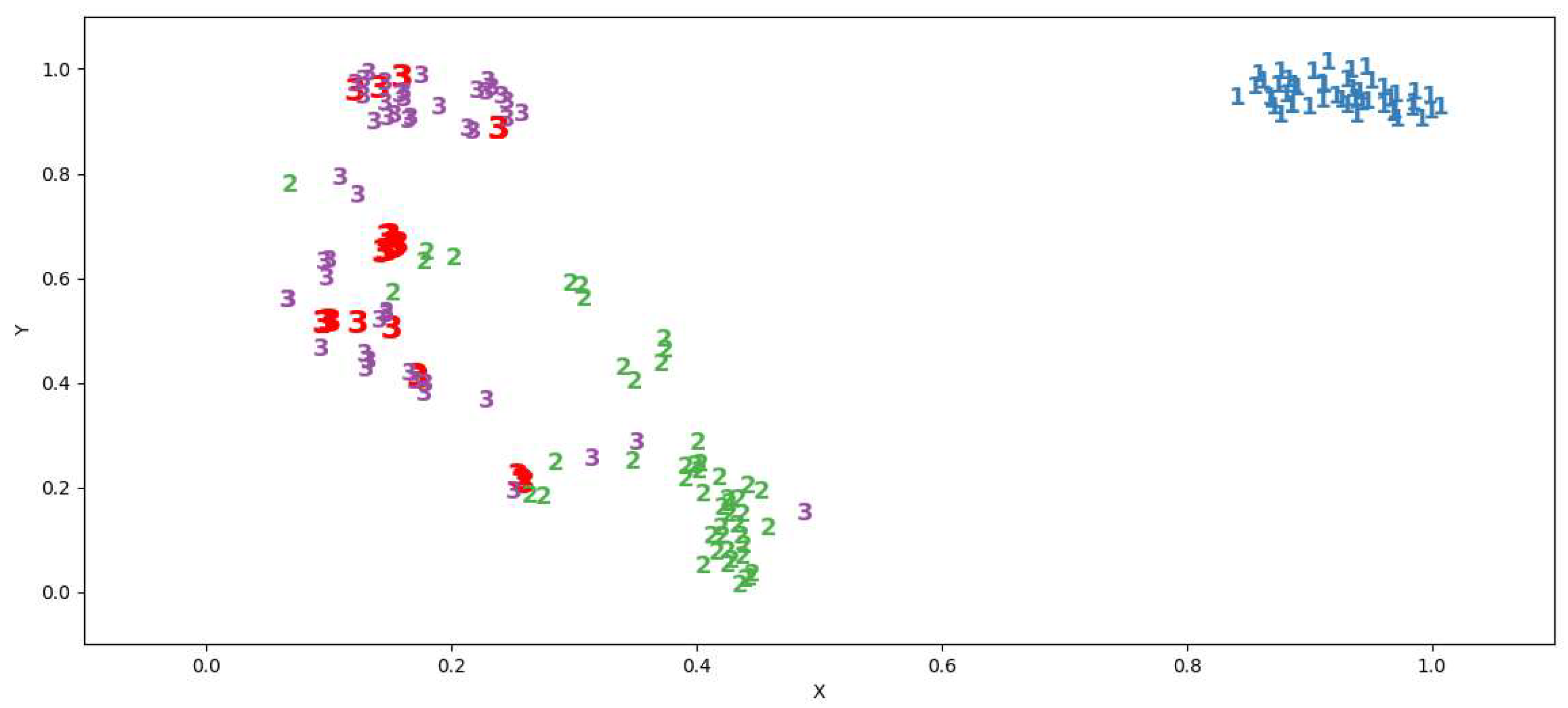
An example of such division of the feature space using an ensemble of auto-encoders based on neural networks is shown in
Figure 6.
Let us calculate the EDCAP characteristics for the considered example and three variants of the classifier, including an ensemble with a common auto-encoder. Since the data set certainly does not contain intersections of the class definition area, the characteristic will be equal to zero.
We present the values of the characteristics
and
of individual classes in
Table 3.
A generalized characteristic of the considered classifiers according to the EDCA criterion is presented in
Table 4.
It is easy to see from the tables that traditional classifiers have the highest value of the Excess characteristic, which means a higher vulnerability to adversarial attacks. A similar conclusion was made earlier based on visual analysis of
Figure 5.
Another important conclusion is the increased resistance of the ensemble of auto-encoders to adversarial attacks, which can be improved with the addition of a common auto-encoder trained on the data of all classes.
3.5. The Synthesis and the Algorithm of an Adversarial Attack-Resistant Classifier
Let us consider the structure, functioning algorithm and synthesis method of the EnAE (Ensemble of Auto-Encoders) multiclass classifier based on an ensemble of neural network auto-encoders. This classifier also includes a general auto-encoder for the union of all classes, which allows the classifier to detect the absence of belonging to known classes. Applying control of the classification area outside the training set based on the EDCAP approach is supposed to make this classifier more resistant to adversarial attacks.
Let us introduce the necessary notation and definitions.
To designate a neural network of the multilayer perceptron type with
inputs, hidden fully connected layers with the number of neurons
and the number of outputs
, we will use the notation:
To designate the Dropout layer, we will indicate the letter
D in the notation:
We will call an auto-encoder a neural network of the multilayer perceptron type with an equal number of inputs and outputs
and more than one hidden layer:
The result of the auto-encoder is a reconstruction error (
RE):
For examples of the training set and similar sets, the reconstruction error should be small, and for other examples it should be large. The training of the auto-encoder on the training set
is carried out according to the criterion of minimizing the reconstruction error:
Setting the reconstruction error threshold
allows one to build a decision rule for a one-class classifier:
A possible way to calculate the threshold is the maximum reconstruction error on the training set:
Let
classes given in the vector space
and described by training sets of samples:
For convenience, let us introduce the training set of samples of all classes:
Suppose there are also test sets for each of the classes:
We will assume that the data and have passed the necessary preprocessing and normalization.
We need to build a classifier that would report the class label for any if is similar to the examples from or 0 if is not similar to any of the classes.
3.5.1. The Synthesis of the EnAE Classifier
The synthesis procedure for the classifier is presented below:
Setting architecture
Training of neural network auto-encoders:
Calculation of the values that determine decision-making:
Threshold calculation for single-class classifier based on
Threshold calculation for single-class classifier based on
Calculation of the quality characteristics of the resulting classifier with details by class:
According to the EDCAP criterion: , , , , ,
By test sets : ,, ,
Analysis of the classification quality characteristics of individual auto-encoders , , , adjusting their architecture, training parameters and repeating steps 2–4 until the required quality level is obtained.
3.5.2. The Algorithm of the EnAE Classifier
The auto-encoder operation algorithm is presented below:
If , then does not belong to any of the classes.
Otherwise, if , then does not belong to any of the classes.
Otherwise, if there is only one such that , then belongs to class .
Otherwise, there are several
such that
, then the example
belongs to the class
for which the relative reconstruction error is minimal:
The proposed synthesis method uses a neural network auto-encoder, however, it is worth noting that a one-class classifier can be implemented based on another machine learning method, for example, SVM. The chosen machine learning method should build a compact region for each class in the feature space.

