
A Transfer Learning Evaluation of Deep Neural Networks for Image Classification


Abstract
:1. Introduction
2. Summary of Related Learning Methods
2.1. Zero-Shot Learning
2.2. One-Shot Leaning
2.3. Few-Shot Learning
2.4. Transfer Learning
3. Models and Datasets
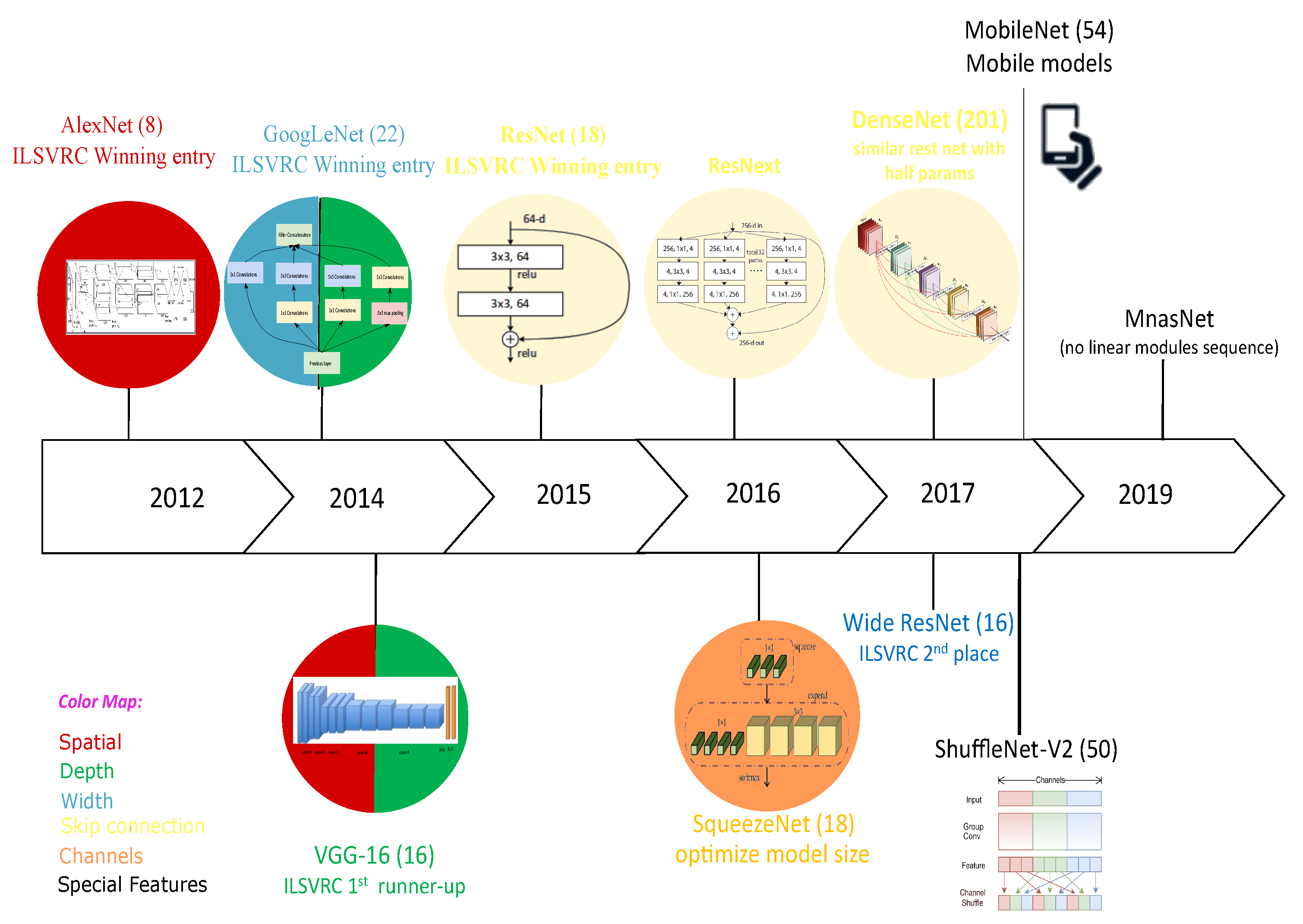
3.1. CNN-Design-Based Architectures
- Depth: The NN depth is represented by the number of successive layers. Theoretically, deep NNs are more efficient than shallow architectures, and increasing the depth of the network by adding hidden layers has a significant effect on supervised learning, particularly for classification tasks [23]. However, cascading layers in a Deep Neural Network (DNN) is not straightforward, and this may cause an exponential increase in the computational cost;
- Width: The width of a CNN is as significant as the depth. Stacking layers may learn various feature representations, but they would not learn useful features. Therefore, a DNN should be wide enough, so the loss at the local minima could be smaller with larger layer widths [24];
- Spatial kernel size: A CNN has many parameters and hyperparameters, including weights, biases, the number of layers, the activation function, the learning rate, and the kernel size, which define the level of granularity. Choosing the kernel size affects the correlation of neighboring pixels. Smaller filters extract local and fine-grained features, whereas larger filters extract coarse-grained features [25];
- Skip connection: Although a deeper NN yields better performance, it may face challenges in performance degradation, vanishing gradients, or higher test and training errors [26]. To tackle these problems, the shortcut layer connection was first proposed by [27] by skipping some intermediate layers to allow the special flow of information across the layers, for example zero-padding, projection, dropout, skip connections, etc.;
- Channels: CNNs have powerful performance in learning features automatically, and this can be dynamically performed by tuning the kernel weights. However, some feature maps have little or no role in object discrimination [28] and could cause overfitting as well. Those feature maps (or the channels) can be optimally selected in designing the CNN to avoid overfitting.
3.2. Neural Network Architectures
3.3. Datasets
3.3.1. Hymenoptera
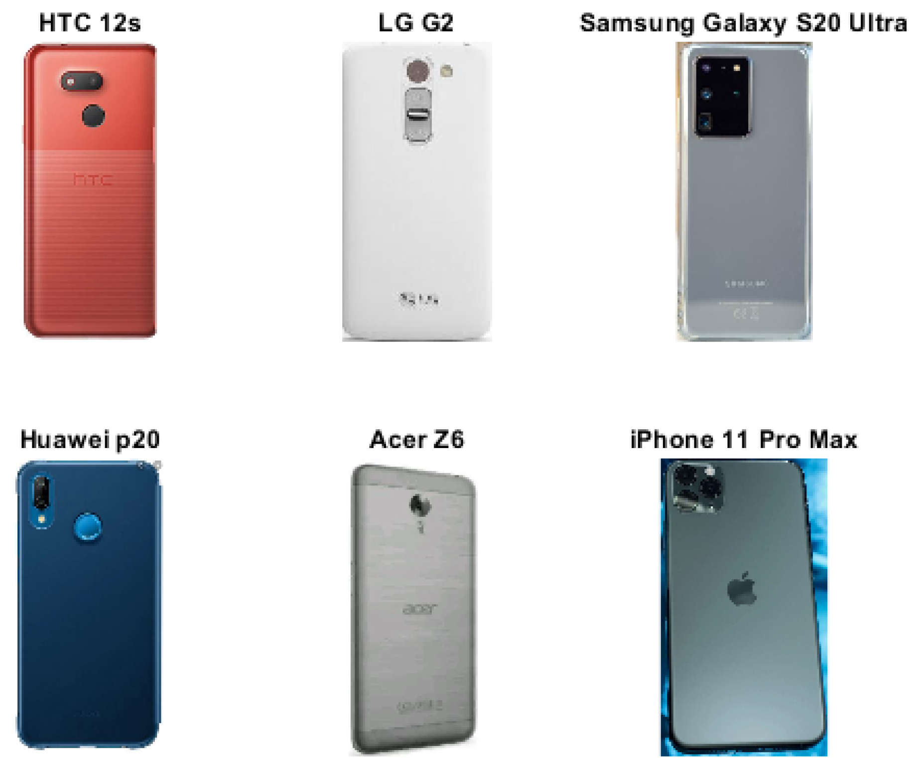
3.3.2. Smartphone Dataset
3.3.3. Augmented Smartphone Dataset
4. Implementation
- Fine-tune the classifier layer only: This method keeps the feature extraction layers from the pre-trained model fixed, so-called frozen. We then re-initialized the task-specific classifier parts, as given by reference in the PyTorch vision model implementations [42], with random values. If the PyTorch model did not have an explicit classifier part, for example the ResNet18 architecture, we fine-tuned only the last fully connected layer. We froze all other weights during training. This technique saved training time and, to some degree, overcame the problem of a small-sized target dataset because it only updated a few weights;
- Fine-tune all layers: For this method, we used the PyTorch vision models with original weights as pre-trained on ImageNet and fine-tuned the entire parameter vector. In theory, this technique achieves higher accuracy and generalization, but it requires a longer training time since it is used for initializing weights by continuing the backpropagation instead of random initialization in scratch training.
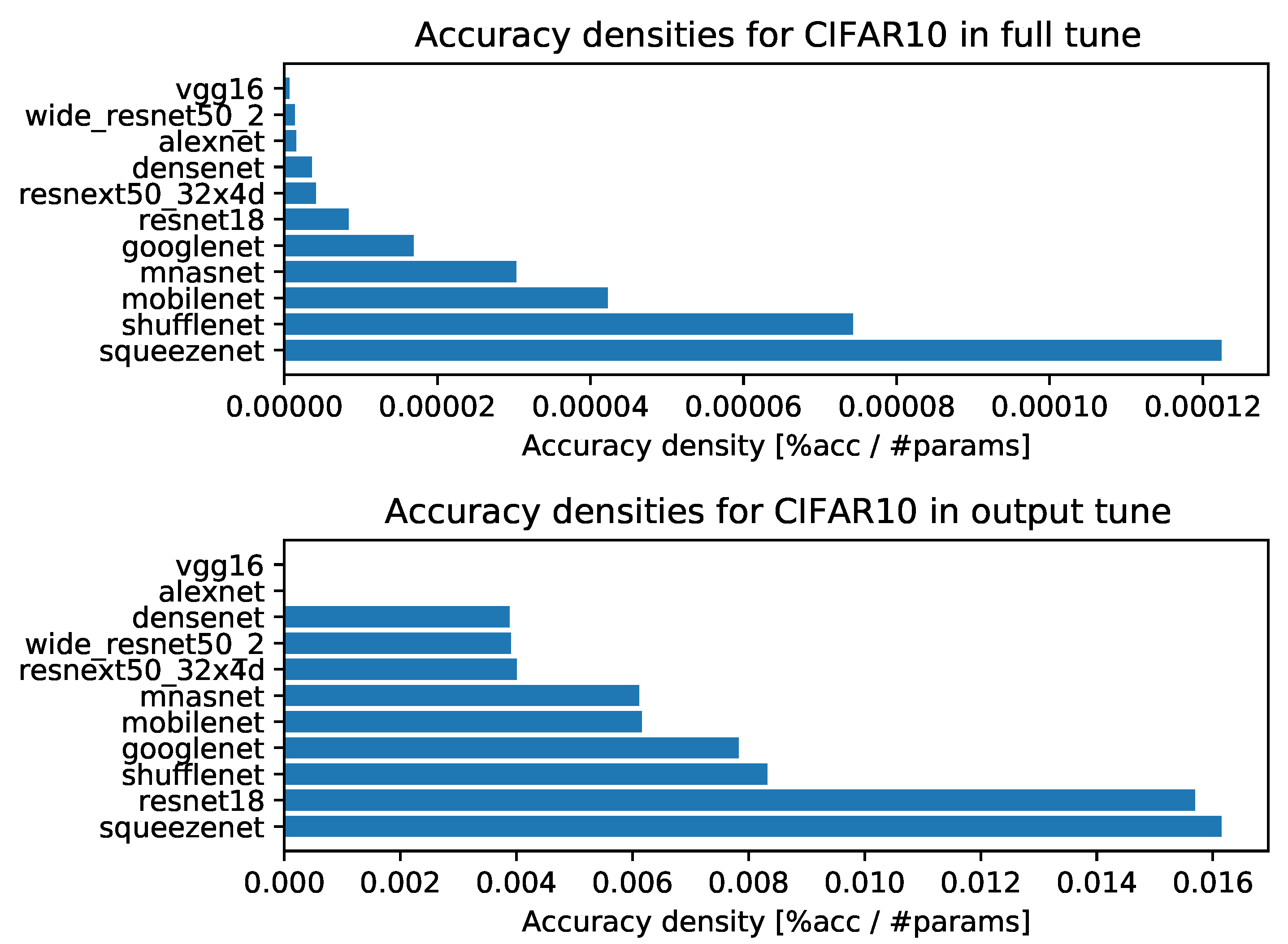
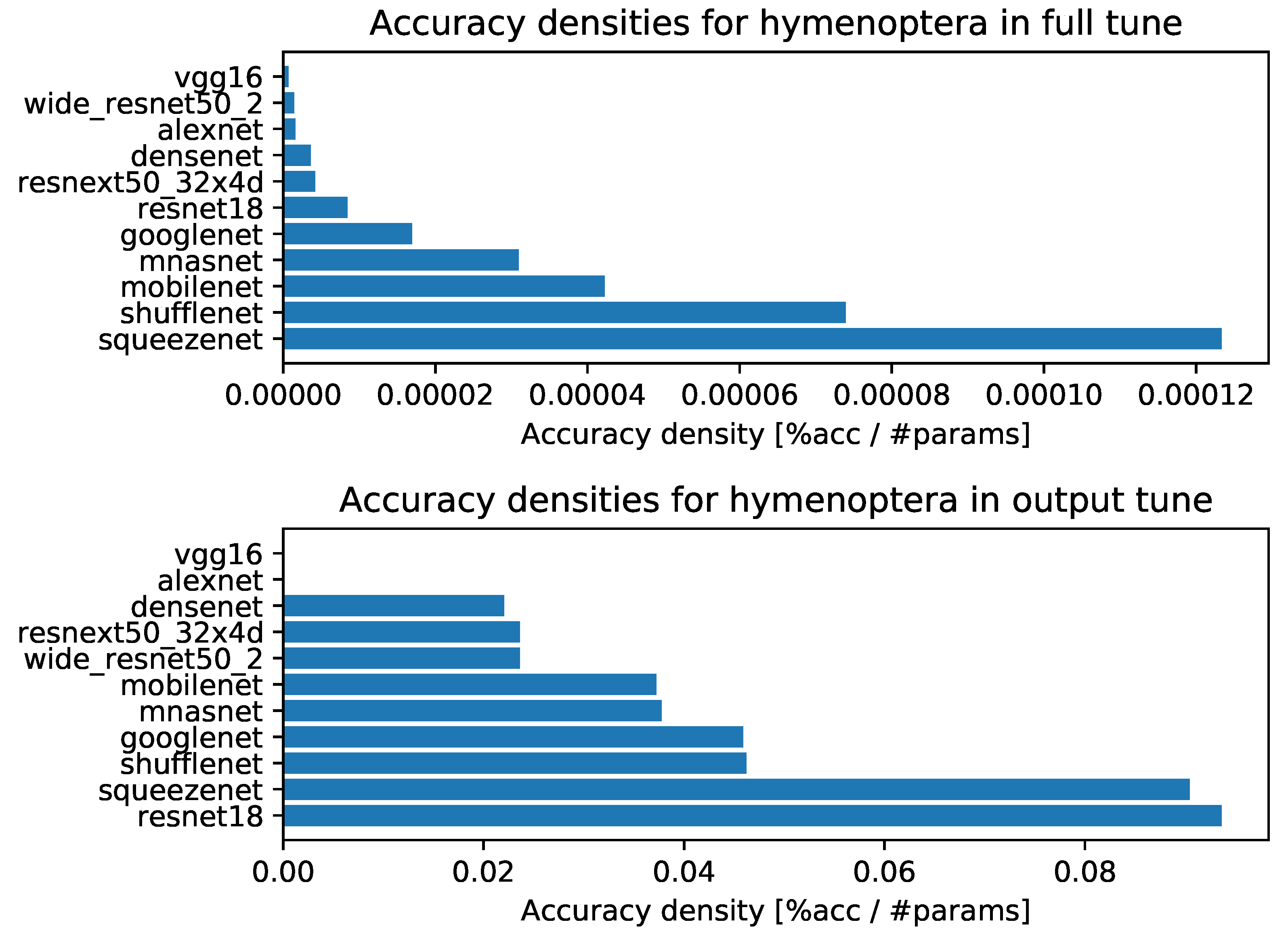
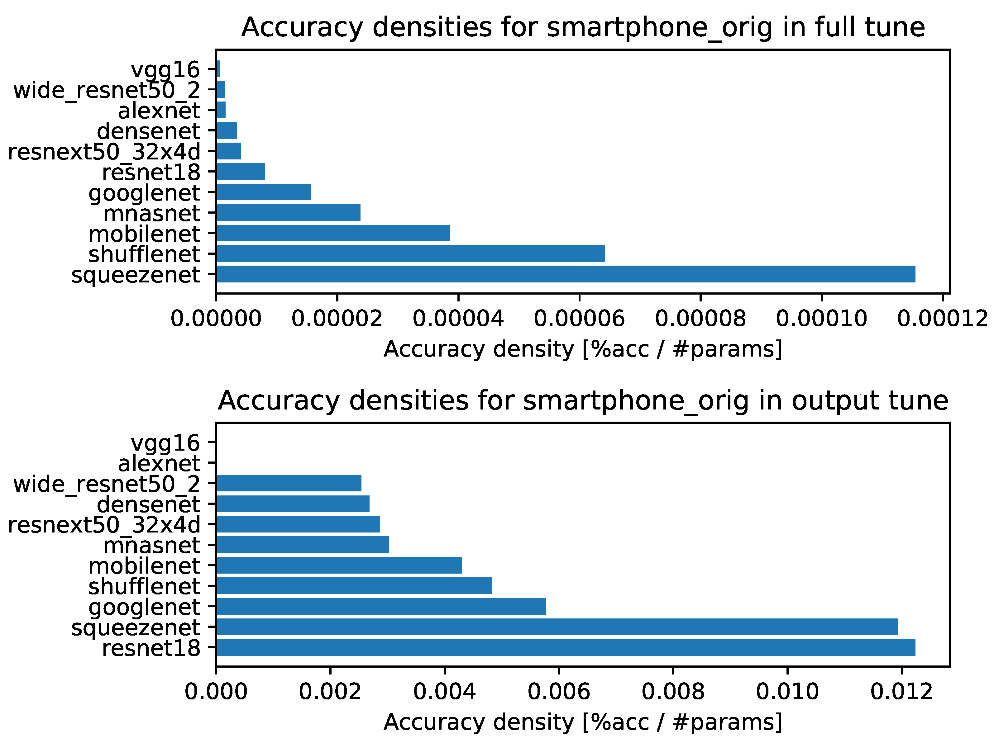
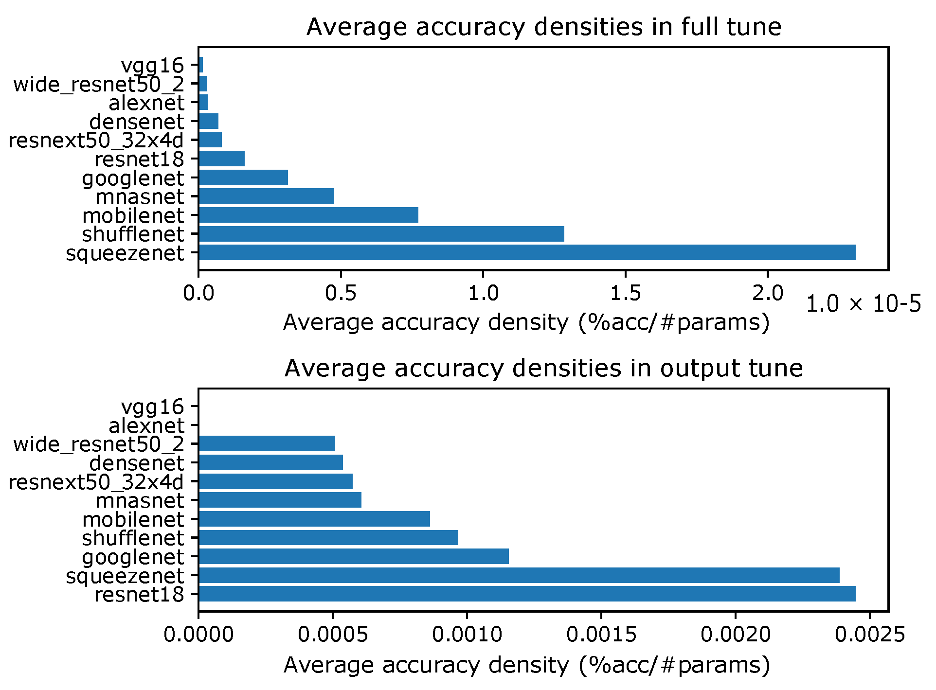
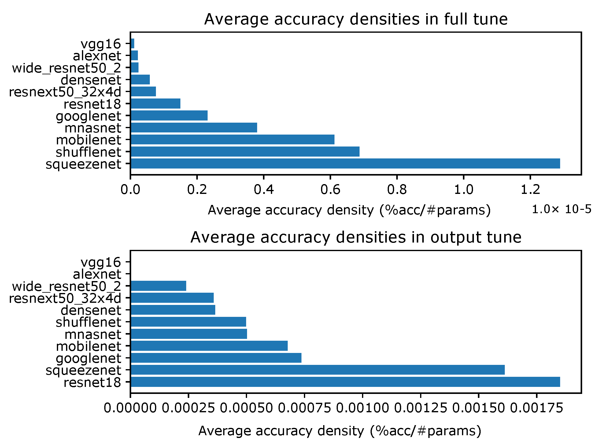
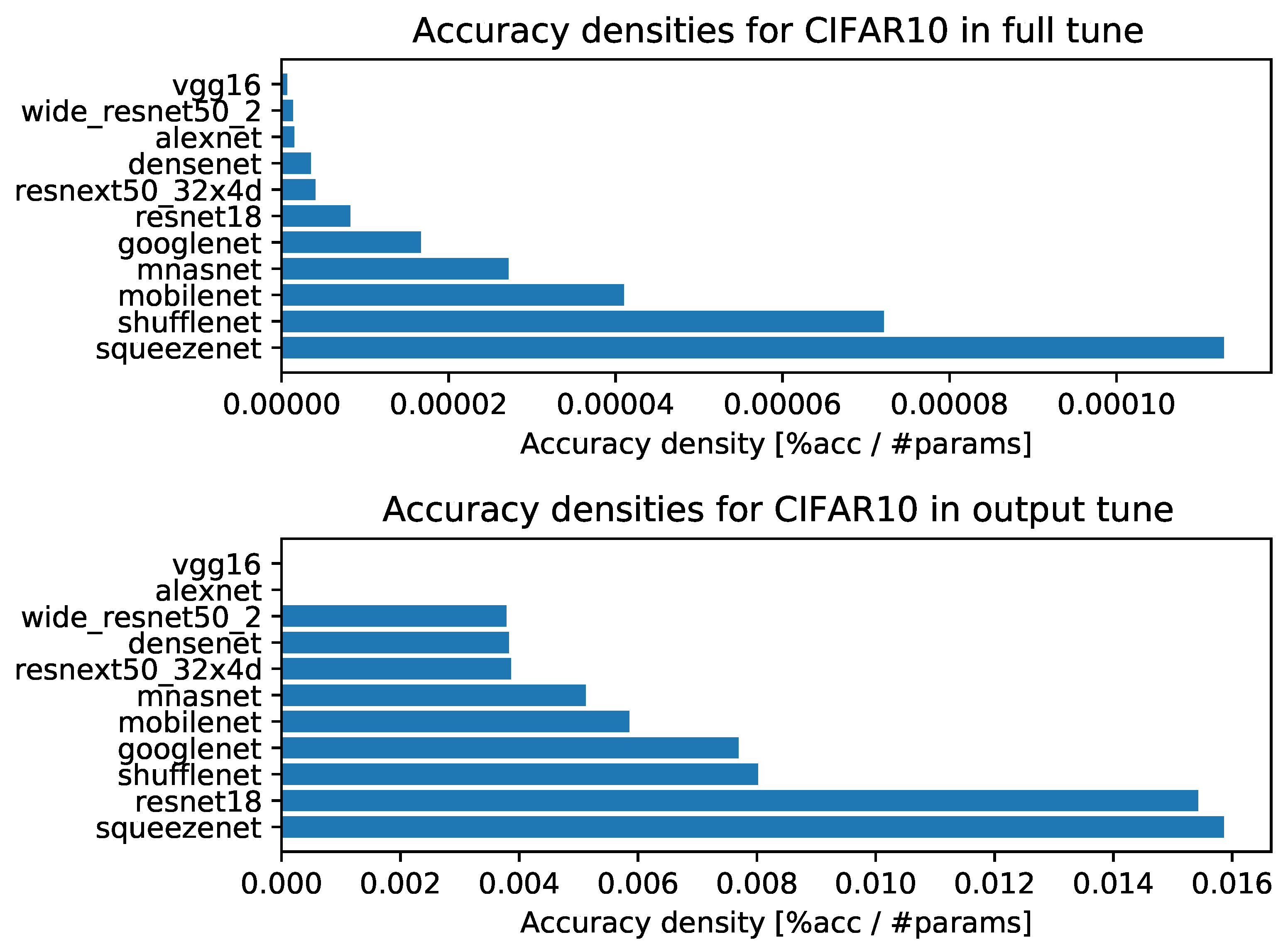
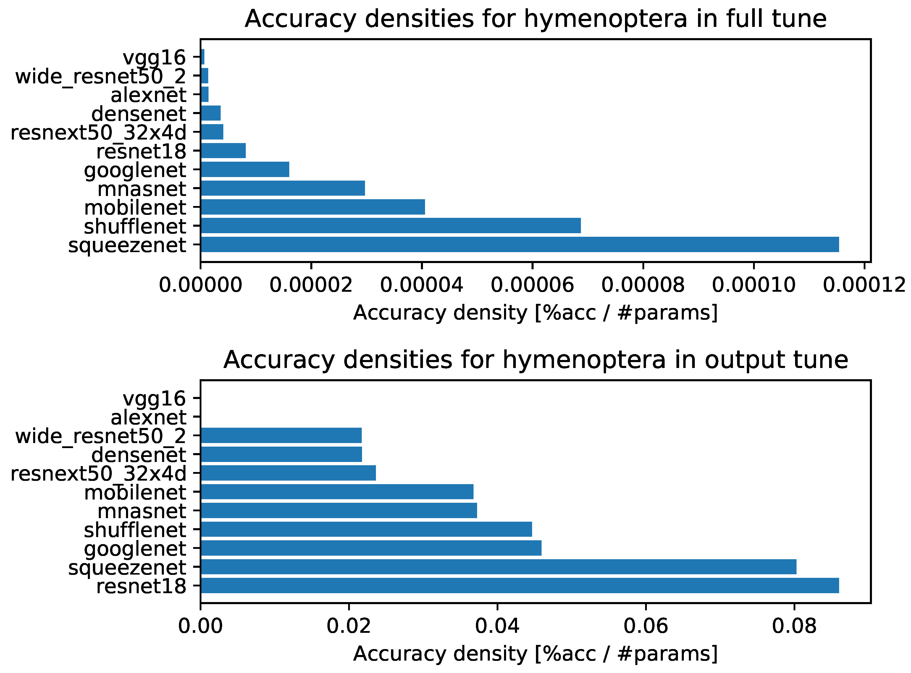
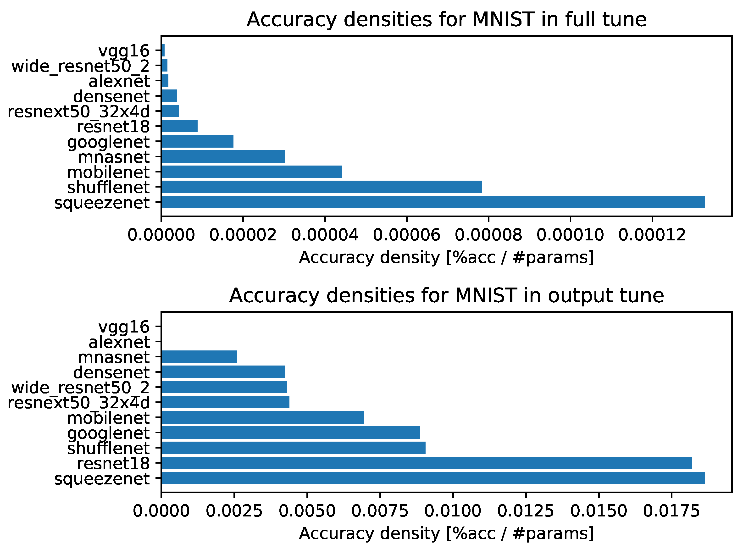
4.1. Accuracy Density
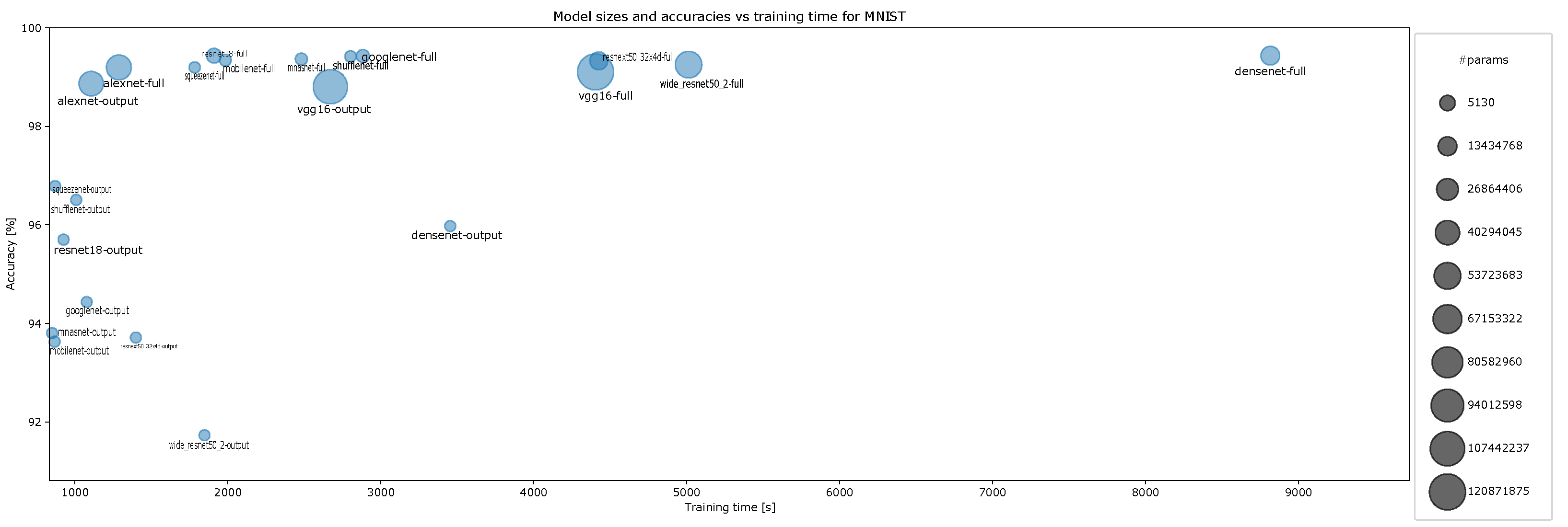
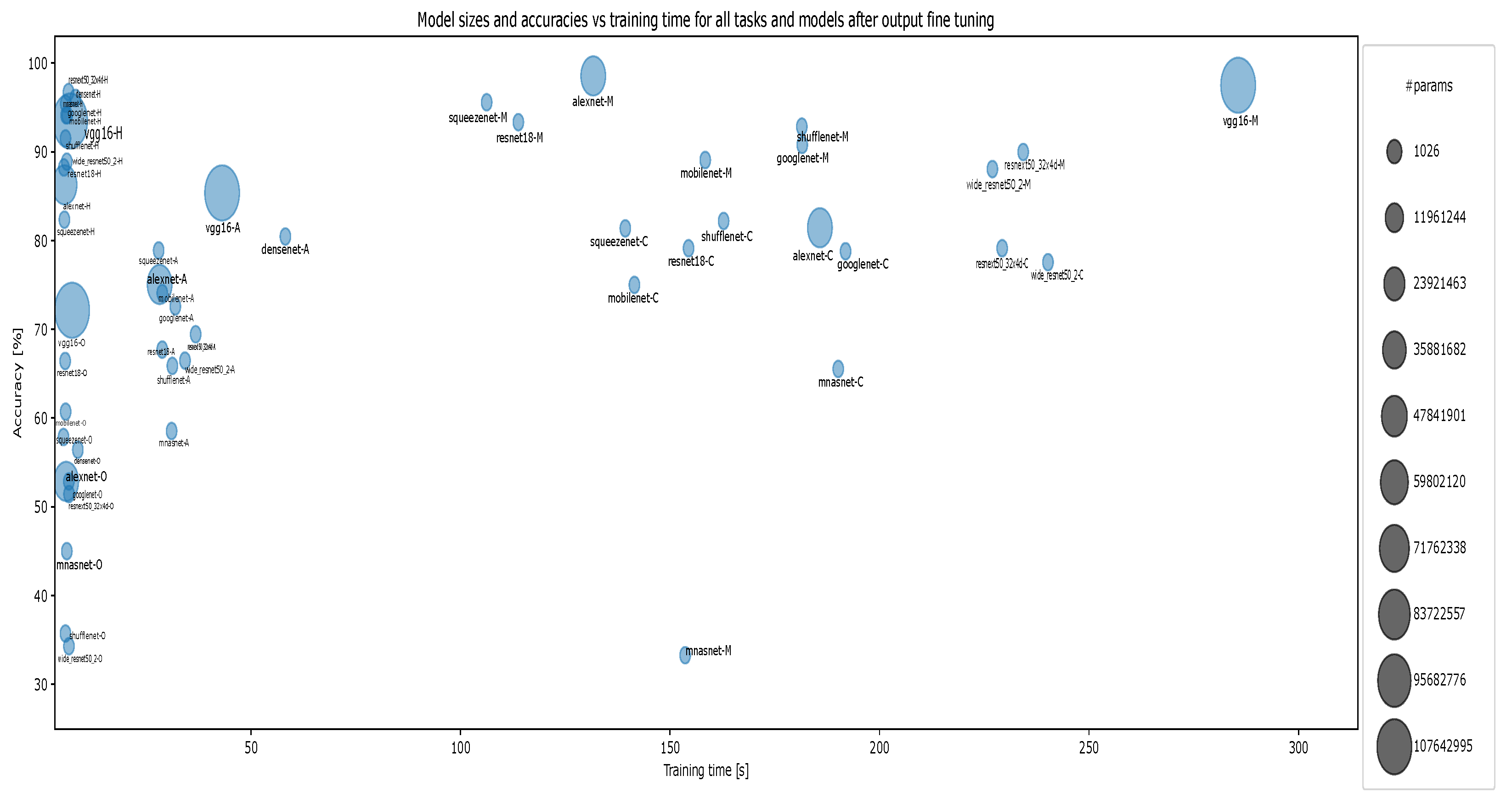
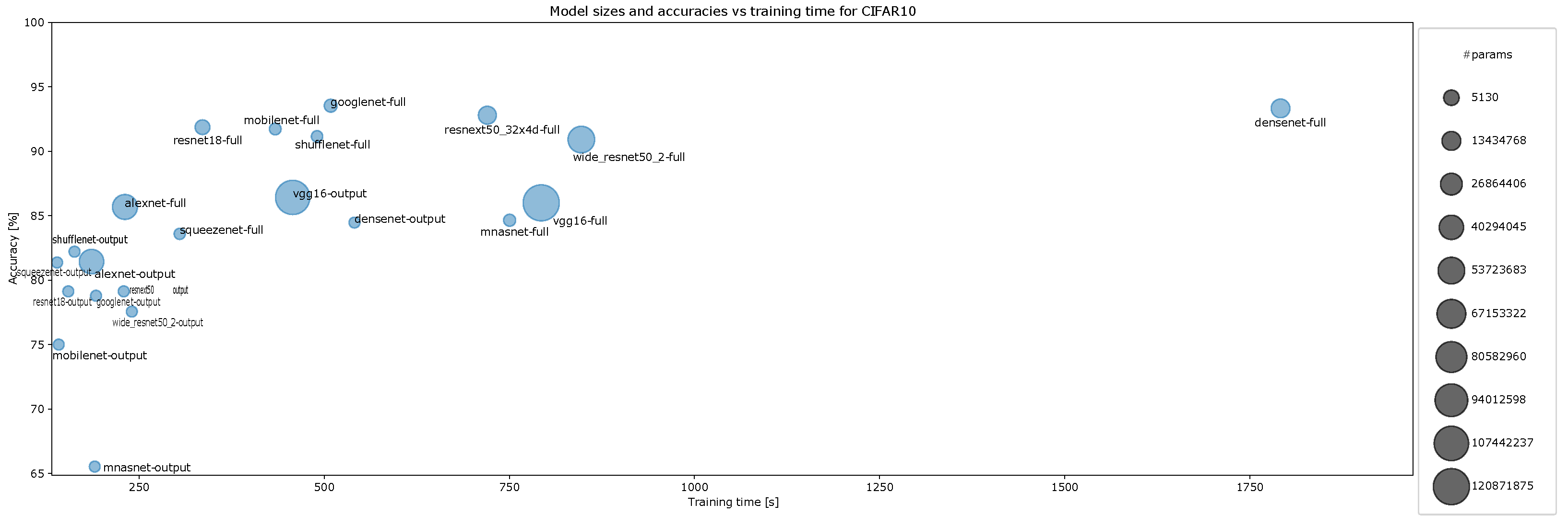
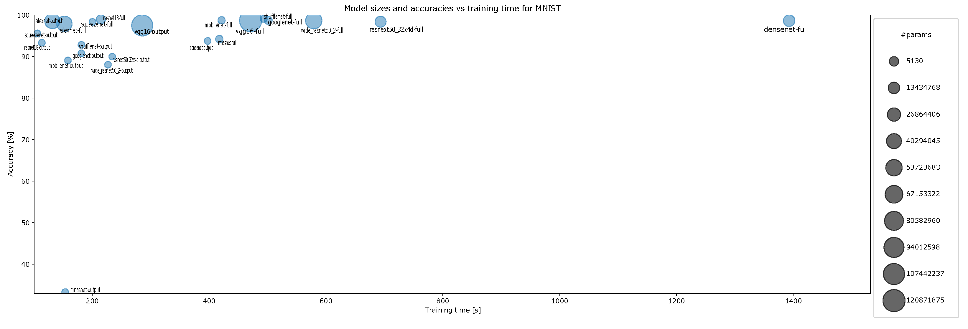
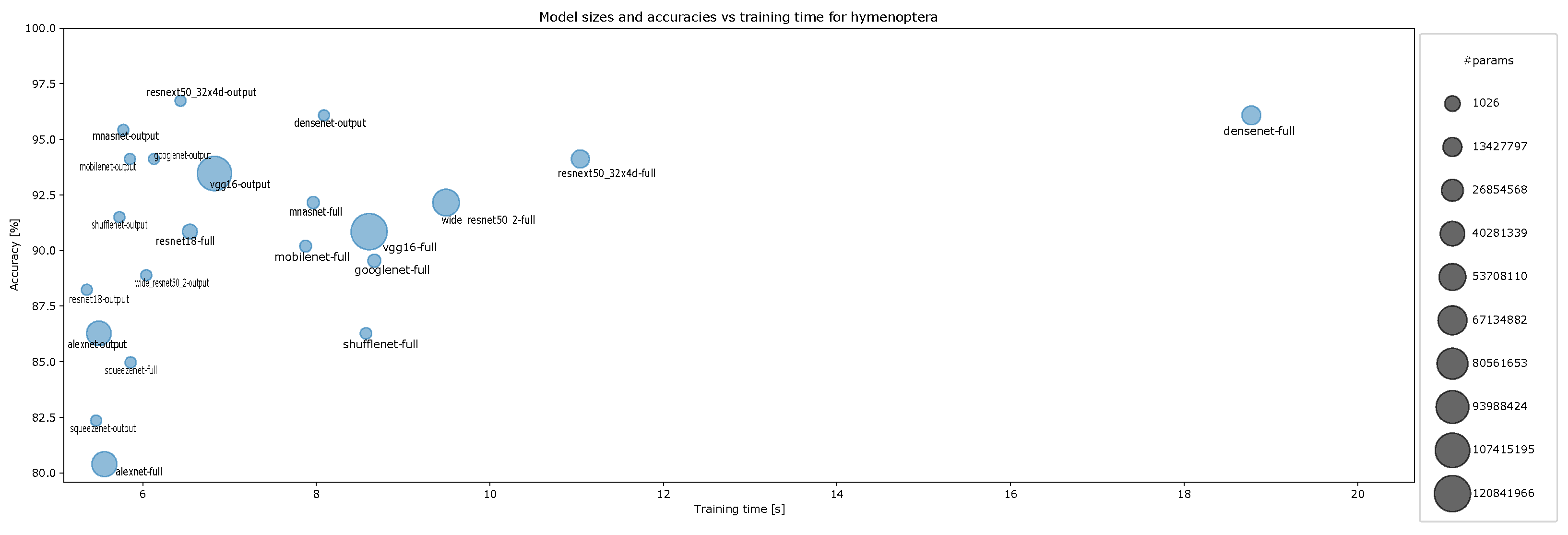
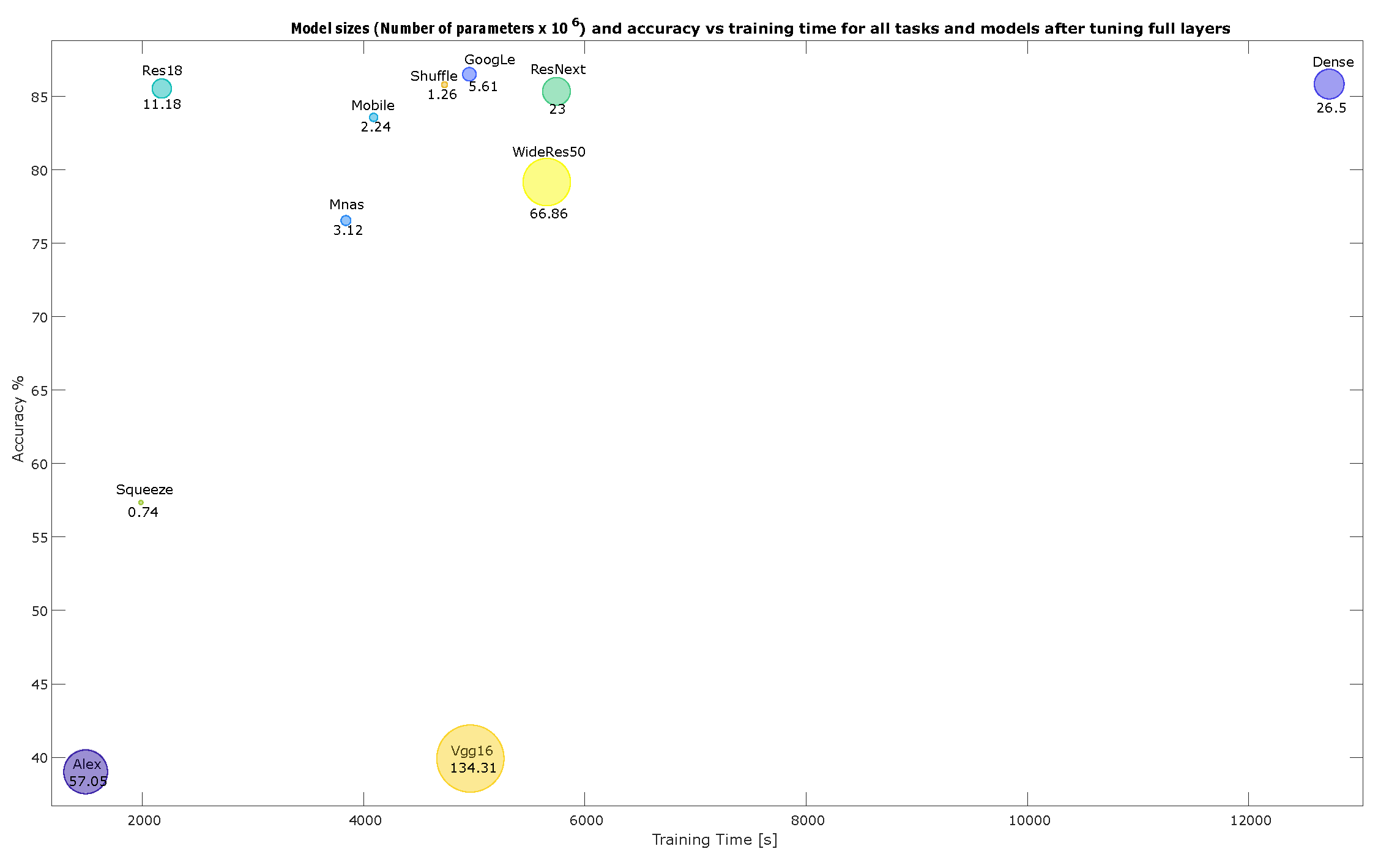
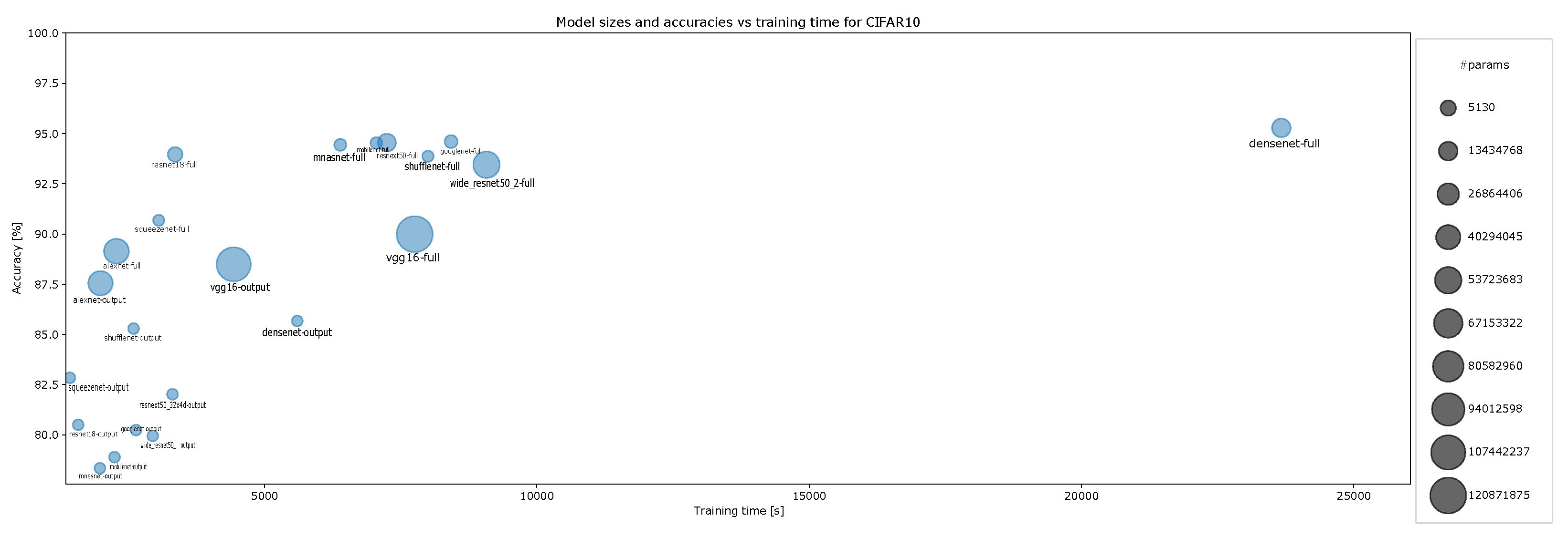
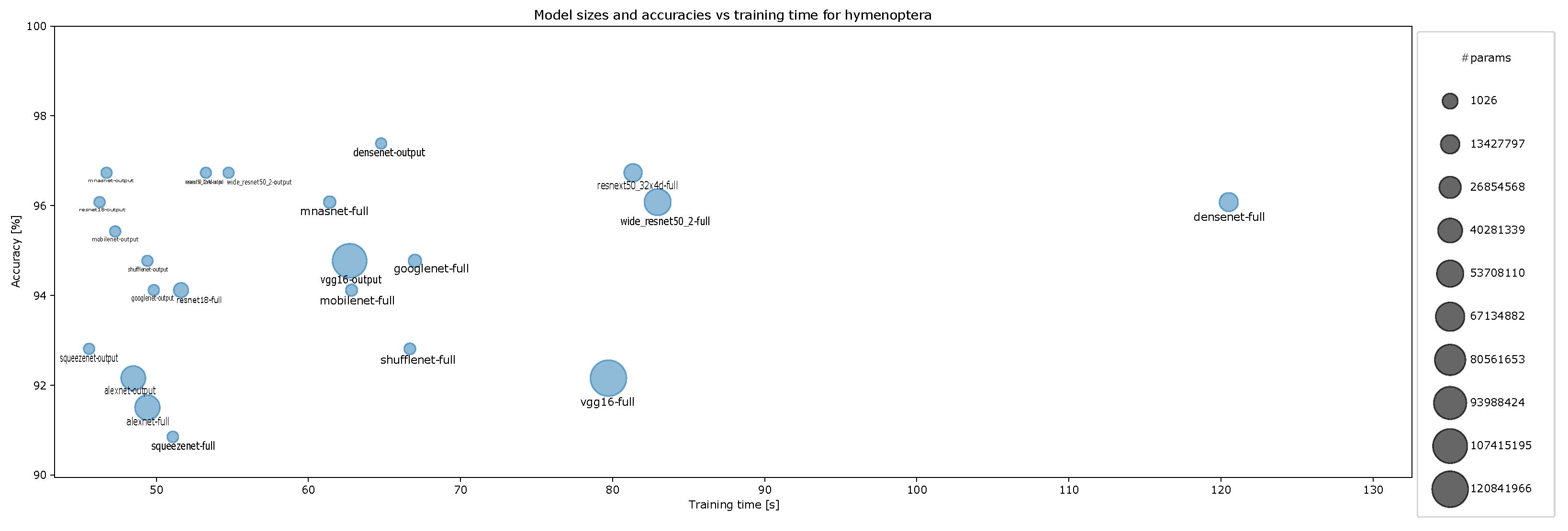
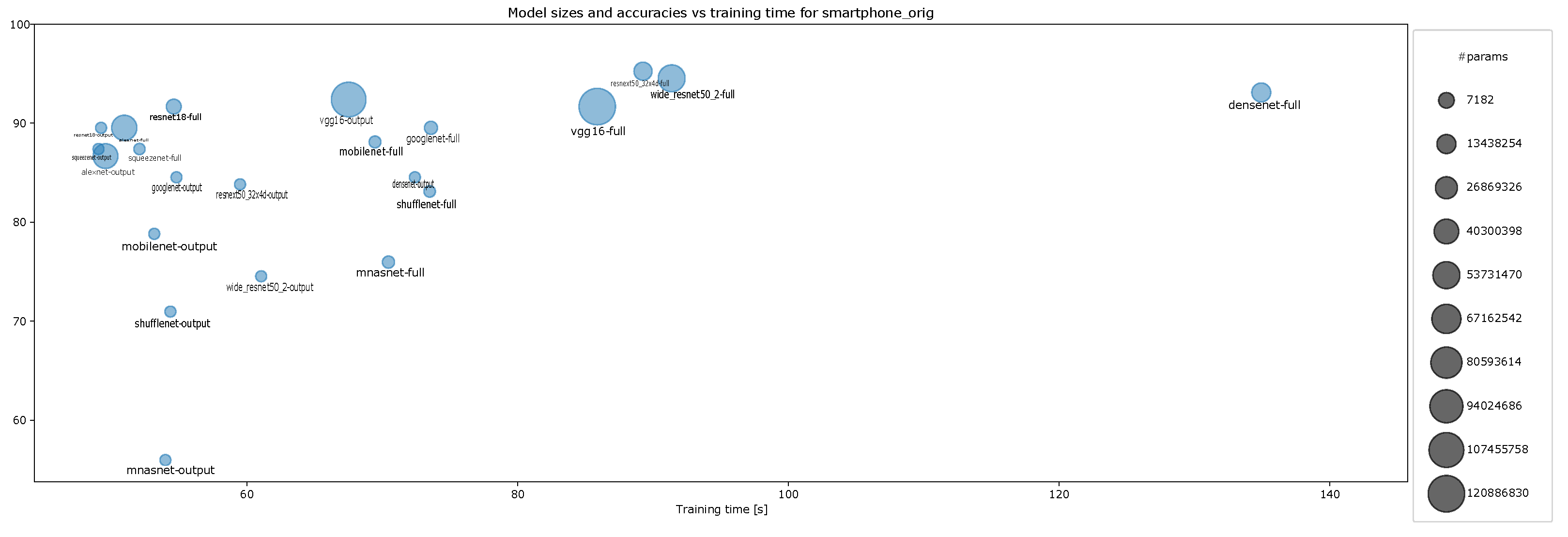
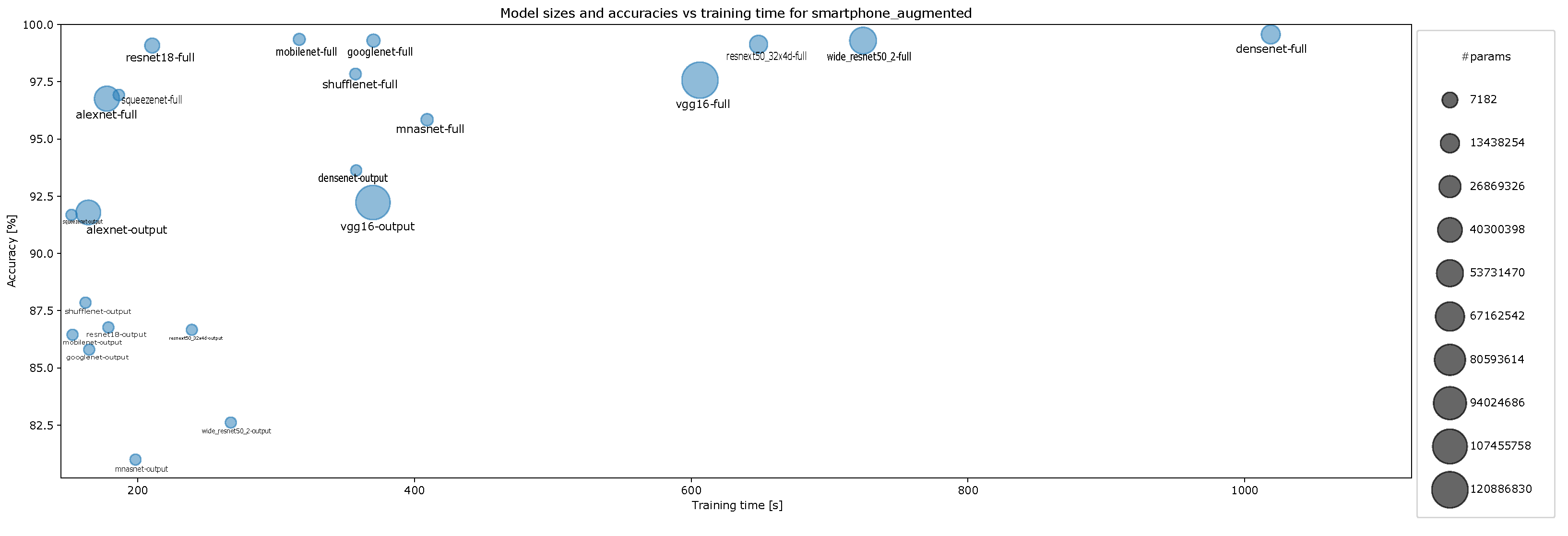
4.2. Accuracy and Model Sizes vs. Training Time
5. Results
5.1. One-Episode Learning
5.1.1. Fine-Tuning the Full Layers
5.1.2. Fine-Tuning the Classifier Layers Only
5.2. Ten-Episode Learning
5.2.1. Fine-Tuning the Full Layers
5.2.2. Fine-Tuning the Classifier Layers Only
6. Conclusions
Author Contributions
Funding
Institutional Review Board Statement
Informed Consent Statement
Data Availability Statement
Conflicts of Interest
Appendix A. Accuracy Densities for Each Task with One-Episode Learning
- Accuracy densities for one-episode learning on CIFAR-10, Figure A1;
- Accuracy densities for one-episode learning on Hymenoptera, Figure A2;
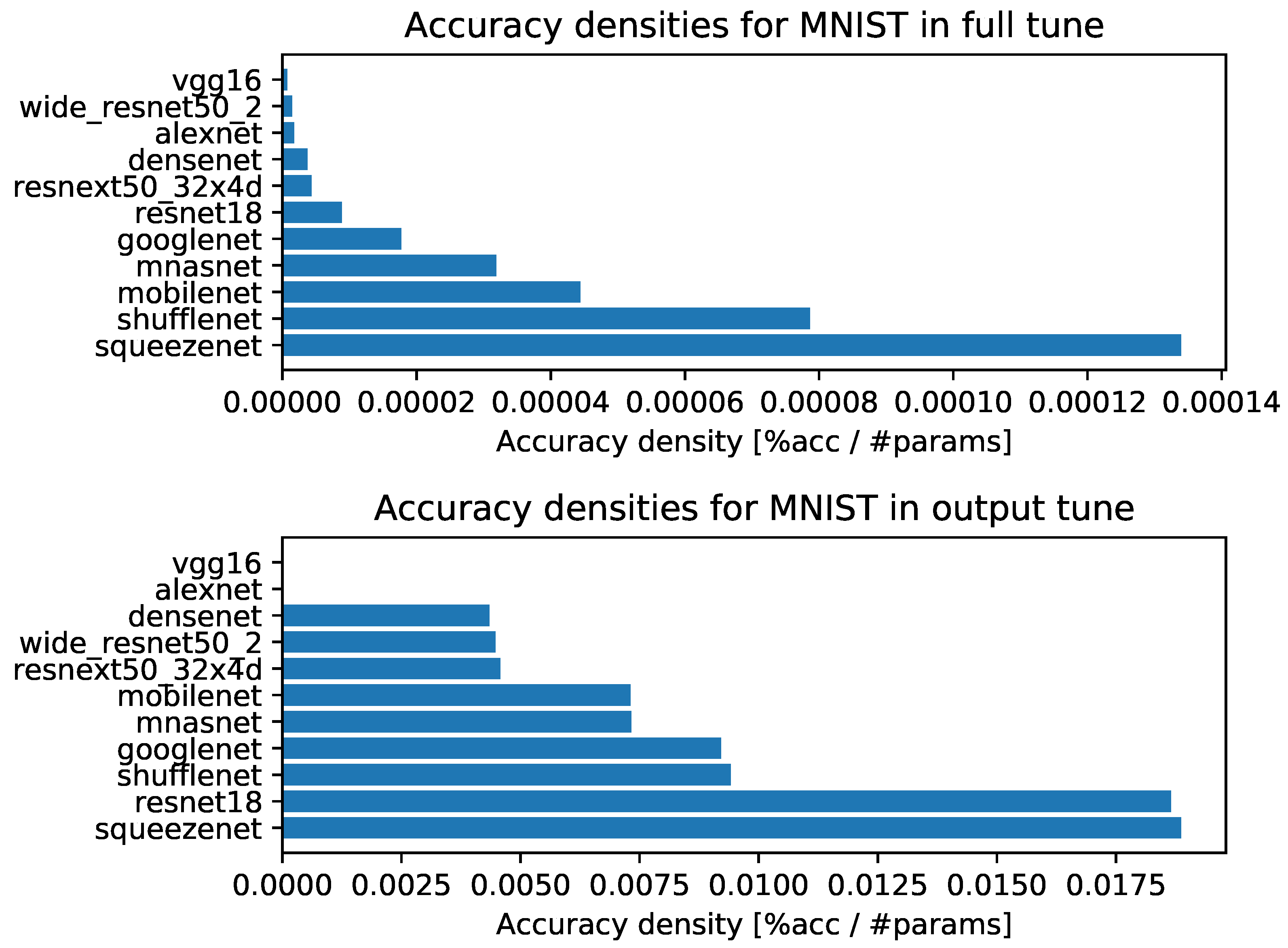
- Accuracy densities for one-episode learning on MNIST, Figure A3;
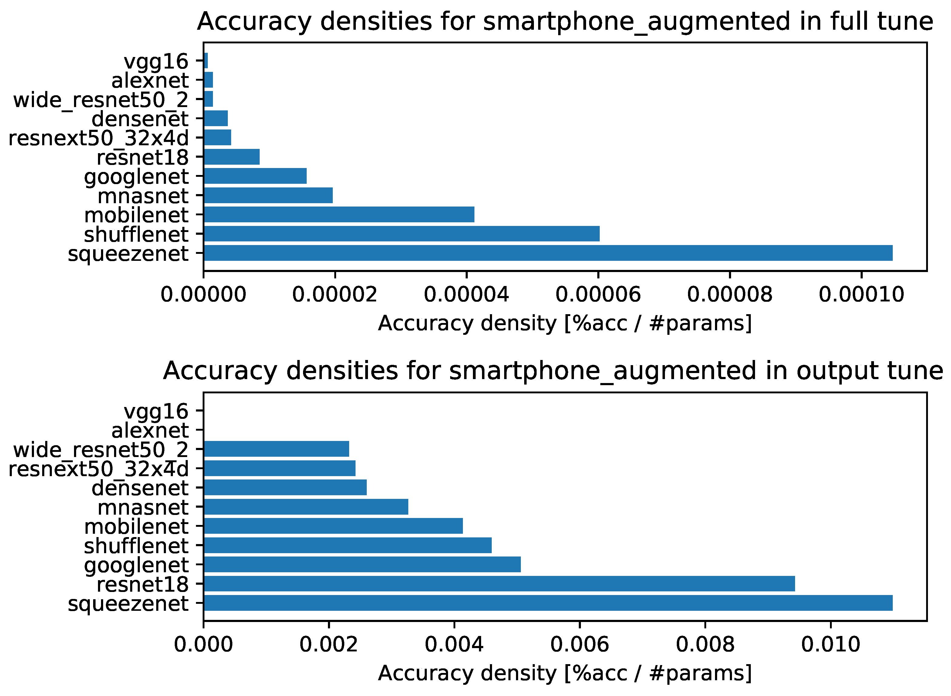
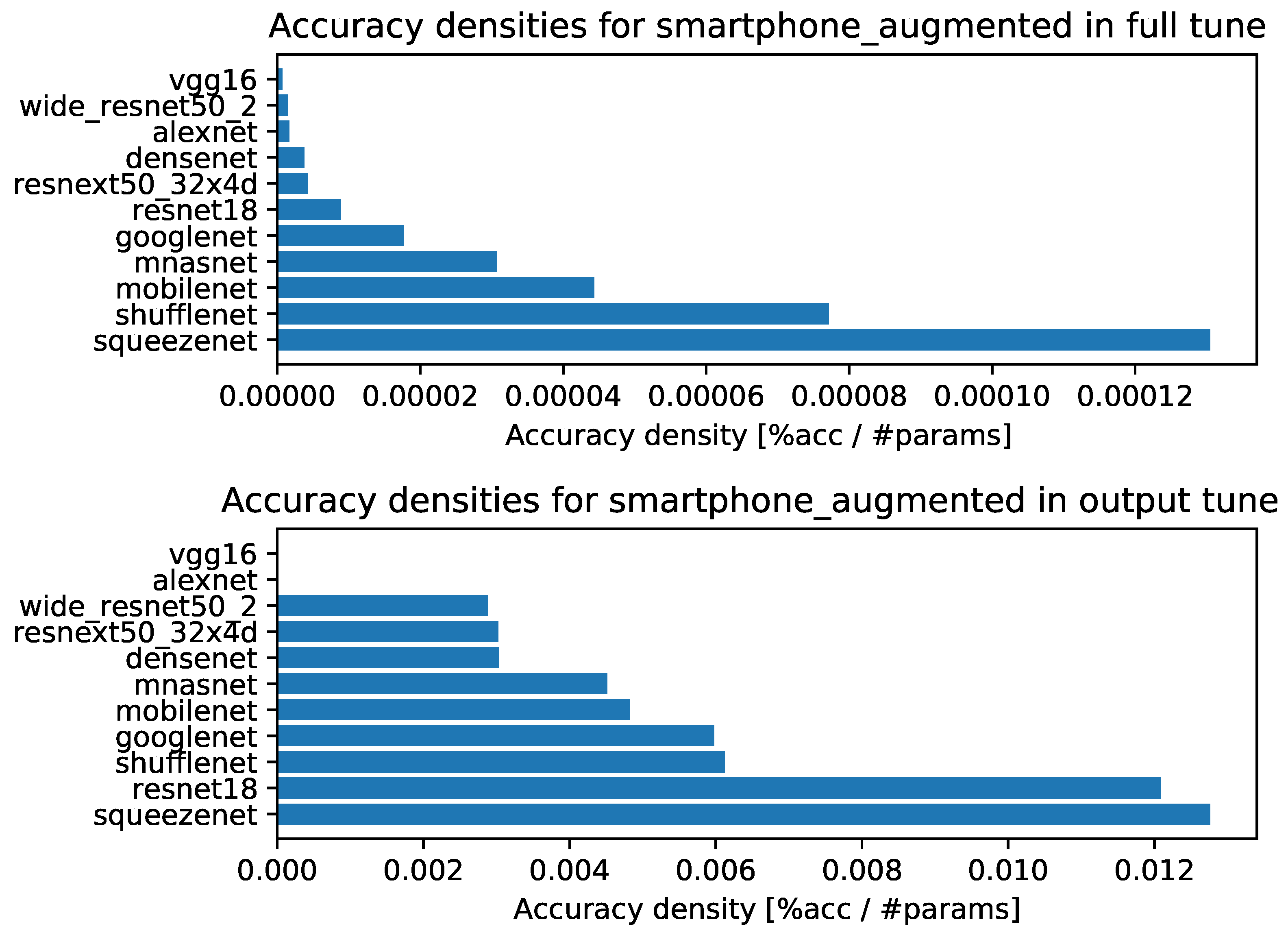
- Accuracy densities for one-episode learning on augmented smartphone data, Figure A4;
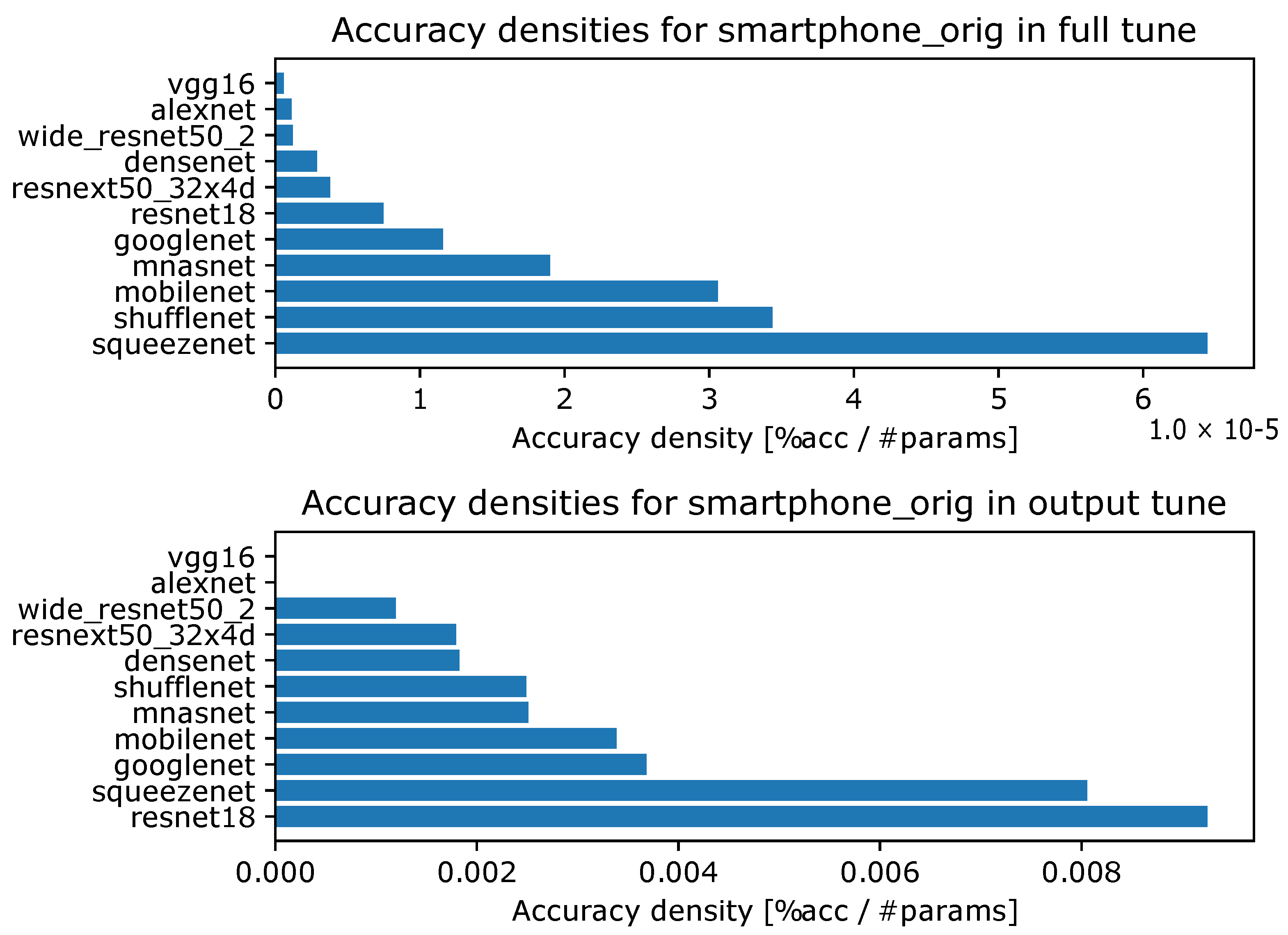
- Accuracy densities for one-episode learning on original smartphone data, Figure A5.


Appendix B. Accuracy Densities for Each Task with Ten-Episode Learning
- Accuracy densities for ten-episode learning on CIFAR-10, Figure A6;
- Accuracy densities for ten-episode learning on Hymenoptera, Figure A7;
- Accuracy densities for ten-episode learning on MNIST, Figure A8;
- Accuracy densities for ten-episode learning on augmented smartphone data, Figure A9;
- Accuracy densities for ten-episode learning on original smartphone data, Figure A10.


Appendix C. Accuracy vs. Training Time and Number of Parameters (Model Size) for Each Task with Ten-Episode Learning
- Accuracy vs. training time and model size for CIFAR-10 for ten-episode training, Figure A11;
- Accuracy vs. training time and model size for MNIST for ten-episode training, Figure A12;
- Accuracy vs. training time and model size for Hymenoptera for ten-episode training, Figure A13;
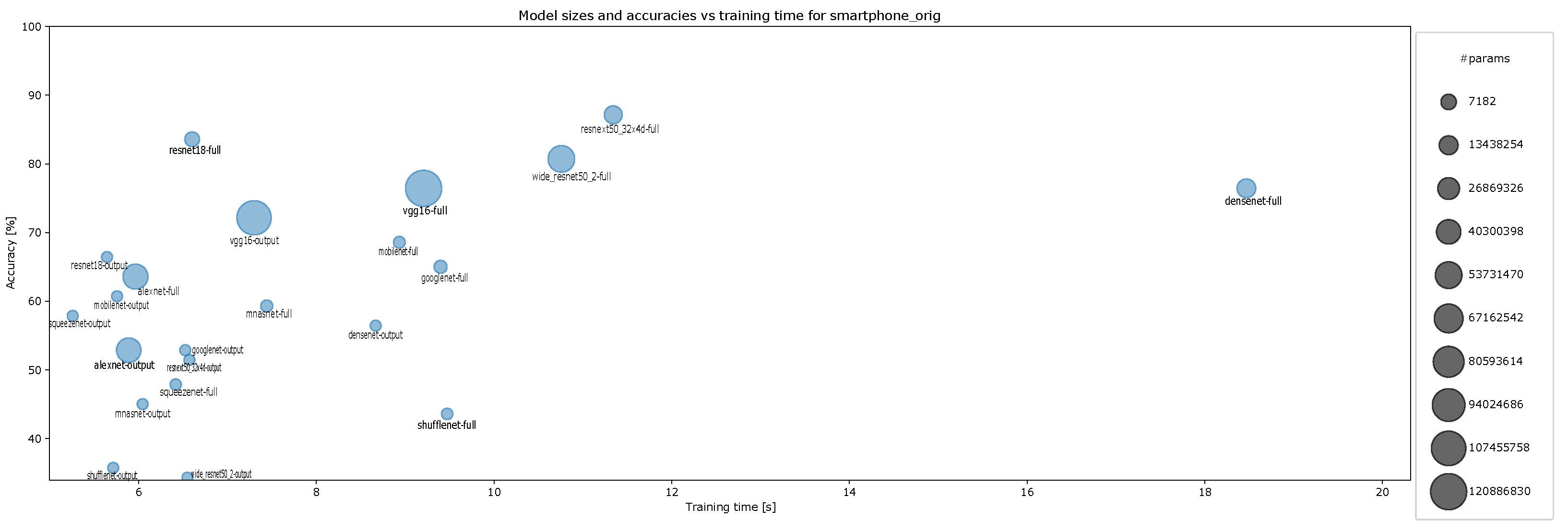
- Accuracy vs. training time and model size for original smartphone data for ten-episode training, Figure A14;
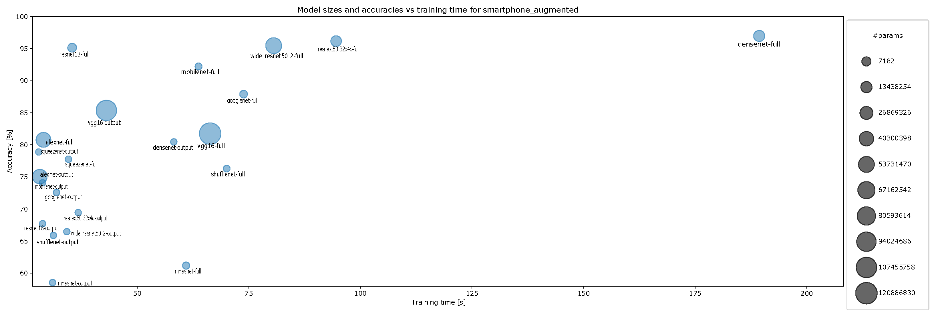
- Accuracy vs. training time and model size for augmented smartphone data for ten-episode training, Figure A15;
- Model sizes and accuracy vs. training time for all tasks and models after fine-tuning the classifier layer only, where A refers to Augmented smartphones, C to CIFAR10, H to Hymenoptera, M to MNIST, and O to the Original smartphone dataset, Figure A16;
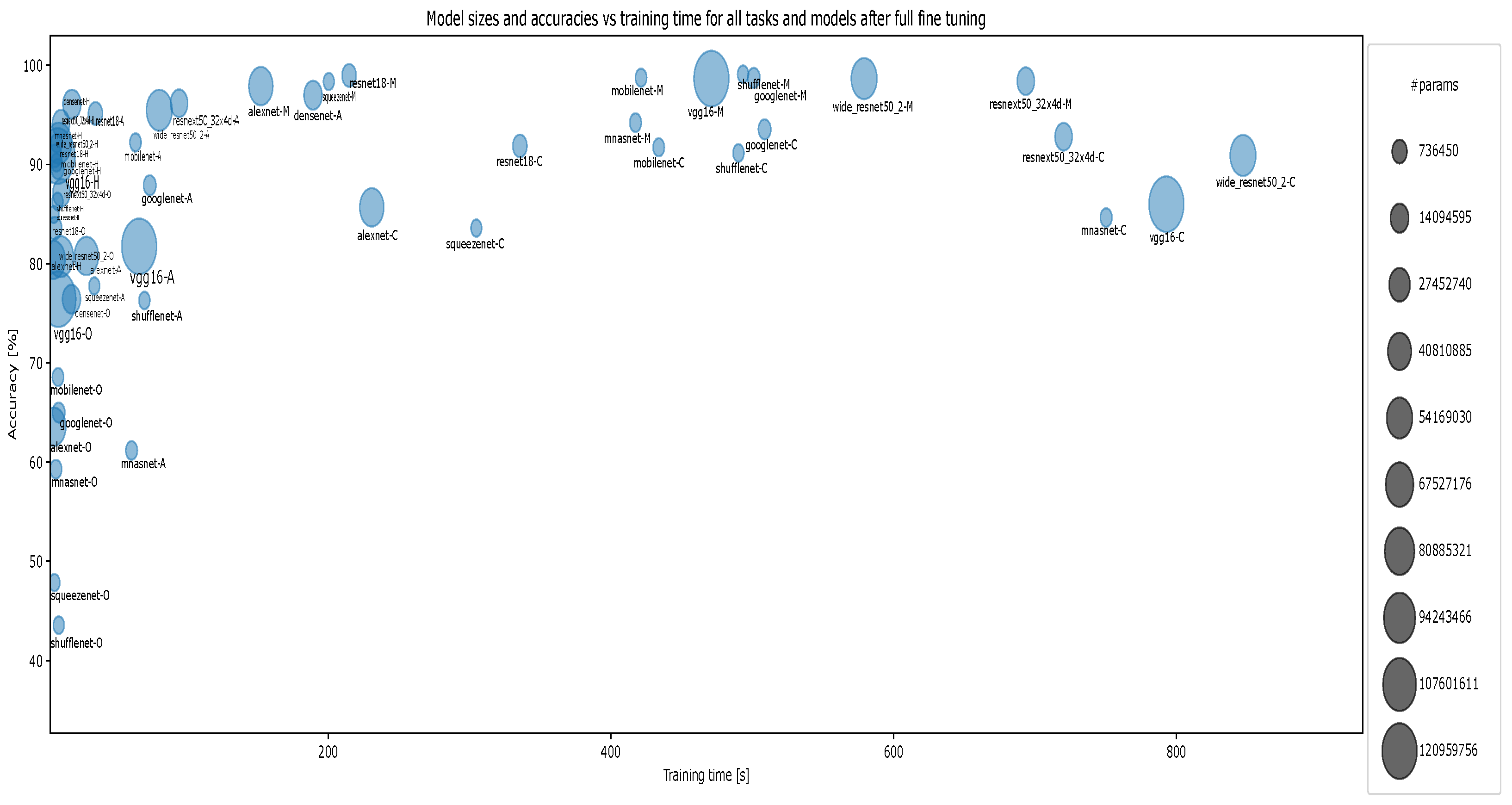
- Model sizes and accuracy vs. training time for all tasks and models after full fine-tuning, where A refers to Augmented smartphones, C to CIFAR10, H to Hymenoptera, M to MNIST, and O to the Original smartphone dataset, Figure A17.


Appendix D. Accuracy vs. Training Time and Model Size for Each Task with One-Episode Learning
- Accuracy vs. training time and model size for CIFAR-10 for one-episode training, Figure A18;
- Accuracy vs. training time and model size for MNIST for one-episode training, Figure A19;
- Accuracy vs. training time and model size for Hymenoptera for one-episode training, Figure A20;
- Accuracy vs. training time and model size for original smartphone data for one-episode training, Figure A21;
- Accuracy vs. training time and model size for augmented smartphone data for one-episode training, Figure A22.


References
- Lundervold, A.S.; Lundervold, A. An overview of deep learning in medical imaging focusing on MRI. Z. Fur Med. Phys. 2019, 29, 102–127. [Google Scholar] [CrossRef] [PubMed]
- Pires de Lima, R.; Marfurt, K. Convolutional Neural Network for Remote-Sensing Scene Classification: Transfer Learning Analysis. Remote Sens. 2020, 12, 86. [Google Scholar] [CrossRef] [Green Version]
- Zou, M.; Zhong, Y. Transfer Learning for Classification of Optical Satellite Image. Sens. Imaging 2018, 19, 6. [Google Scholar] [CrossRef]
- Abou Baker, N.; Szabo-Müller, P.; Handmann, U. Feature-fusion transfer learning method as a basis to support automated smartphone recycling in a circular smart city. In Proceedings of the EAI S-CUBE 2020—11th EAI International Conference on Sensor Systems and Software, Aalborg, Denmark, 10–11 December 2020. [Google Scholar]
- Houlsby, N.; Giurgiu, A.; Jastrzebski, S.; Morrone, B.; de Laroussilhe, Q.; Gesmundo, A.; Attariyan, M.; Gelly, S. Parameter-Efficient Transfer Learning for NLP. arXiv 2019, arXiv:1902.00751. [Google Scholar]
- Choe, D.; Choi, E.; Kim, D.K. The Real-Time Mobile Application for Classifying of Endangered Parrot Species Using the CNN Models Based on Transfer Learning. Mob. Inf. Syst. 2020, 2020, 1–13. [Google Scholar] [CrossRef]
- Ismail Fawaz, H.; Forestier, G.; Weber, J.; Idoumghar, L.; Muller, P.A. Transfer learning for time series classification. In Proceedings of the 2018 IEEE International Conference on Big Data (Big Data), Seattle, WA, USA, 10–13 December 2018. [Google Scholar] [CrossRef] [Green Version]
- Canziani, A.; Paszke, A.; Culurciello, E. An Analysis of Deep Neural Network Models for Practical Applications. arXiv 2017, arXiv:1605.07678. [Google Scholar]
- Bianco, S.; Cadene, R.; Celona, L.; Napoletano, P. Benchmark Analysis of Representative Deep Neural Network Architectures. IEEE Access 2018, 6, 64270–64277. [Google Scholar] [CrossRef]
- Socher, R.; Ganjoo, M.; Sridhar, H.; Bastani, O.; Manning, C.D.; Ng, A.Y. Zero-Shot Learning Through Cross-Modal Transfer. arXiv 2013, arXiv:1301.3666. [Google Scholar]
- Xian, Y.; Schiele, B.; Akata, Z. Zero-Shot Learning—The Good, the Bad and the Ugly. arXiv 2020, arXiv:1703.04394. [Google Scholar]
- Lampert, C.H.; Nickisch, H.; Harmeling, S. Attribute-Based Classification for Zero-Shot Visual Object Categorization. IEEE Trans. Pattern Anal. Mach. Intell. 2014, 36, 453–465. [Google Scholar] [CrossRef]
- Zhang, Z.; Saligrama, V. Zero-Shot Learning via Semantic Similarity Embedding. arXiv 2015, arXiv:1509.04767. [Google Scholar]
- Akata, Z.; Perronnin, F.; Harchaoui, Z.; Schmid, C. Label-Embedding for Image Classification. IEEE Trans. Pattern Anal. Mach. Intell. 2016, 38, 1425–1438. [Google Scholar] [CrossRef] [PubMed] [Green Version]
- Bart, E.; Ullman, S. Cross-generalization: Learning novel classes from a single example by feature replacement. In Proceedings of the 2005 IEEE Computer Society Conference on Computer Vision and Pattern Recognition (CVPR’05), San Diego, CA, USA, 20–26 June 2005; Volume 1, pp. 672–679. [Google Scholar] [CrossRef]
- Fink, M. Object Classification from a Single Example Utilizing Class Relevance Metrics. In Advances in Neural Information Processing Systems; Saul, L., Weiss, Y., Bottou, L., Eds.; MIT Press: Cambridge, MA, USA, 2005; Volume 17. [Google Scholar]
- Tommasi, T.; Caputo, B. The More You Know, the Less You Learn: From Knowledge Transfer to One-shot Learning of Object Categories. In Proceedings of the BMVC, London, UK, 7–10 September 2009; Available online: http://www.bmva.org/bmvc/2009/Papers/Paper353/Paper353.html (accessed on 30 November 2021).
- Wang, Y.; Yao, Q.; Kwok, J.T.; Ni, L.M. Generalizing from a Few Examples: A Survey on Few-Shot Learning. ACM Comput. Surv. 2020, 53, 63. [Google Scholar] [CrossRef]
- Azadi, S.; Fisher, M.; Kim, V.; Wang, Z.; Shechtman, E.; Darrell, T. Multi-Content GAN for Few-Shot Font Style Transfer. arXiv 2017, arXiv:1712.00516. [Google Scholar]
- Liu, B.; Wang, X.; Dixit, M.; Kwitt, R.; Vasconcelos, N. Feature Space Transfer for Data Augmentation. arXiv 2019, arXiv:1801.04356. [Google Scholar]
- Luo, Z.; Zou, Y.; Hoffman, J.; Fei-Fei, L. Label Efficient Learning of Transferable Representations across Domains and Tasks. arXiv 2017, arXiv:1712.00123. [Google Scholar]
- Tan, W.C.; Chen, I.M.; Pantazis, D.; Pan, S.J. Transfer Learning with PipNet: For Automated Visual Analysis of Piping Design. In Proceedings of the 2018 IEEE 14th International Conference on Automation Science and Engineering (CASE), Munich, Germany, 20–24 August 2018; pp. 1296–1301. [Google Scholar] [CrossRef]
- Montúfar, G.; Pascanu, R.; Cho, K.; Bengio, Y. On the Number of Linear Regions of Deep Neural Networks. arXiv 2014, arXiv:1402.1869. [Google Scholar]
- Kawaguchi, K.; Huang, J.; Kaelbling, L.P. Effect of Depth and Width on Local Minima in Deep Learning. Neural Comput. 2019, 31, 1462–1498. [Google Scholar] [CrossRef]
- Khan, A.; Sohail, A.; Zahoora, U.; Qureshi, A.S. A survey of the recent architectures of deep convolutional neural networks. Artif. Intell. Rev. 2020, 53, 5455–5516. [Google Scholar] [CrossRef] [Green Version]
- Hochreiter, S. The Vanishing Gradient Problem during Learning Recurrent Neural Nets and Problem Solutions. Int. J. Uncertain. Fuzziness Knowl.-Based Syst. 1998, 6, 107–116. [Google Scholar] [CrossRef] [Green Version]
- Srivastava, R.K.; Greff, K.; Schmidhuber, J. Highway Networks. arXiv 2015, arXiv:1505.00387. [Google Scholar]
- Hu, J.; Shen, L.; Sun, G. Squeeze-and-Excitation Networks. In Proceedings of the 2018 IEEE/CVF Conference on Computer Vision and Pattern Recognition, Salt Lake City, UT, USA, 18–22 June 2018; pp. 7132–7141. [Google Scholar] [CrossRef] [Green Version]
- Krizhevsky, A.; Sutskever, I.; Hinton, G.E. ImageNet Classification with Deep Convolutional Neural Networks. Adv. Neural Inf. Process. Syst. 2012, 25, 1097–1105. [Google Scholar] [CrossRef]
- Simonyan, K.; Zisserman, A. Very Deep Convolutional Networks for Large-Scale Image Recognition. arXiv 2014, arXiv:1409.1556. [Google Scholar]
- Szegedy, C.; Liu, W.; Jia, Y.; Sermanet, P.; Reed, S.; Anguelov, D.; Erhan, D.; Vanhoucke, V.; Rabinovich, A. Going deeper with convolutions. In Proceedings of the 2015 IEEE Conference on Computer Vision and Pattern Recognition (CVPR), Boston, MA, USA, 7–12 June 2015; pp. 1–9. [Google Scholar] [CrossRef] [Green Version]
- He, K.; Zhang, X.; Ren, S.; Sun, J. Deep Residual Learning for Image Recognition. arXiv 2015, arXiv:1512.03385. [Google Scholar]
- Iandola, F.N.; Han, S.; Moskewicz, M.W.; Ashraf, K.; Dally, W.J.; Keutzer, K. SqueezeNet: AlexNet-level accuracy with 50x fewer parameters and <0.5MB model size. arXiv 2016, arXiv:1602.07360. [Google Scholar]
- Xie, S.; Girshick, R.; Dollar, P.; Tu, Z.; He, K. Aggregated Residual Transformations for Deep Neural Networks. In Proceedings of the 2017 IEEE Conference on Computer Vision and Pattern Recognition (CVPR), Honolulu, HI, USA, 21–26 July 2017; pp. 5987–5995. [Google Scholar] [CrossRef] [Green Version]
- Huang, G.; Liu, Z.; van der Maaten, L.; Weinberger, K.Q. Densely Connected Convolutional Networks. In Proceedings of the 2017 IEEE Conference on Computer Vision and Pattern Recognition (CVPR), Honolulu, HI, USA, 21–26 July 2017; pp. 2261–2269. [Google Scholar] [CrossRef] [Green Version]
- Howard, A.G.; Zhu, M.; Chen, B.; Kalenichenko, D.; Wang, W.; Weyand, T.; Andreetto, M.; Adam, H. MobileNets: Efficient Convolutional Neural Networks for Mobile Vision Applications. arXiv 2017, arXiv:1704.04861. [Google Scholar]
- Zagoruyko, S.; Komodakis, N. Wide Residual Networks. arXiv 2017, arXiv:1605.07146. [Google Scholar]
- Zhang, X.; Zhou, X.; Lin, M.; Sun, J. ShuffleNet: An Extremely Efficient Convolutional Neural Network for Mobile Devices. arXiv 2017, arXiv:1707.01083. [Google Scholar]
- Tan, M.; Chen, B.; Pang, R.; Vasudevan, V.; Sandler, M.; Howard, A.; Le, Q.V. MnasNet: Platform-Aware Neural Architecture Search for Mobile. arXiv 2019, arXiv:1807.11626. [Google Scholar]
- Zaheer, R.; Shaziya, H. A Study of the Optimization Algorithms in Deep Learning. In Proceedings of the 2019 Third International Conference on Inventive Systems and Control (ICISC), Coimbatore, India, 10–11 January 2019; pp. 536–539. [Google Scholar] [CrossRef]
- Kaziha, O.; Bonny, T. A Comparison of Quantized Convolutional and LSTM Recurrent Neural Network Models Using MNIST. In Proceedings of the 2019 International Conference on Electrical and Computing Technologies and Applications (ICECTA), Ras Al Khaimah, United Arab Emirates, 19–21 November 2019; pp. 1–5. [Google Scholar] [CrossRef]
- Paszke, A.; Gross, S.; Massa, F.; Lerer, A.; Bradbury, J.; Chanan, G.; Killeen, T.; Lin, Z.; Gimelshein, N.; Antiga, L.; et al. PyTorch: An Imperative Style, High-Performance Deep Learning Library. Adv. Neural Inf. Process. Syst. 2019, 32, 8024–8035. [Google Scholar]
- Baker, N.A.; Szabo-Mýller, P.; Handmann, U. Transfer learning-based method for automated e-waste recycling in smart cities. EAI Endorsed Trans. Smart Cities 2021, 5. [Google Scholar] [CrossRef]
- Chen, L.; Li, S.; Bai, Q.; Yang, J.; Jiang, S.; Miao, Y. Review of Image Classification Algorithms Based on Convolutional Neural Networks. Remote Sens. 2021, 13, 4712. [Google Scholar] [CrossRef]


| Model | Year | Depth | Main Design Characteristics | Reference |
|---|---|---|---|---|
| AlexNet | 2012 | 8 | Spatial | [29] |
| VGG-16 | 2014 | 16 | Spatial and depth | [30] |
| GoogLeNet | 2014 | 22 | Depth and width | [31] |
| ResNet-18 | 2015 | 18 | Skip connection | [32] |
| SqueezeNet | 2016 | 18 | Channels | [33] |
| ResNext | 2016 | 101 | Skip connection | [34] |
| DenseNet | 2017 | 201 | Skip connection | [35] |
| MobileNet | 2017 | 54 | Depthwise separable conv * | [36] |
| WideResNet | 2017 | 16 | Width | [37] |
| ShuffleNet-V2 | 2017 | 50 | Channel shuffle * | [38] |
| MnasNet | 2019 | No linear sequence | Neural architecture search * | [39] |
Publisher’s Note: MDPI stays neutral with regard to jurisdictional claims in published maps and institutional affiliations. |
© 2022 by the authors. Licensee MDPI, Basel, Switzerland. This article is an open access article distributed under the terms and conditions of the Creative Commons Attribution (CC BY) license (https://creativecommons.org/licenses/by/4.0/).
Share and Cite
Abou Baker, N.; Zengeler, N.; Handmann, U. A Transfer Learning Evaluation of Deep Neural Networks for Image Classification. Mach. Learn. Knowl. Extr. 2022, 4, 22-41. https://doi.org/10.3390/make4010002
Abou Baker N, Zengeler N, Handmann U. A Transfer Learning Evaluation of Deep Neural Networks for Image Classification. Machine Learning and Knowledge Extraction. 2022; 4(1):22-41. https://doi.org/10.3390/make4010002
Chicago/Turabian StyleAbou Baker, Nermeen, Nico Zengeler, and Uwe Handmann. 2022. "A Transfer Learning Evaluation of Deep Neural Networks for Image Classification" Machine Learning and Knowledge Extraction 4, no. 1: 22-41. https://doi.org/10.3390/make4010002
APA StyleAbou Baker, N., Zengeler, N., & Handmann, U. (2022). A Transfer Learning Evaluation of Deep Neural Networks for Image Classification. Machine Learning and Knowledge Extraction, 4(1), 22-41. https://doi.org/10.3390/make4010002