Semantic Predictive Coding with Arbitrated Generative Adversarial Networks


Abstract
1. Introduction
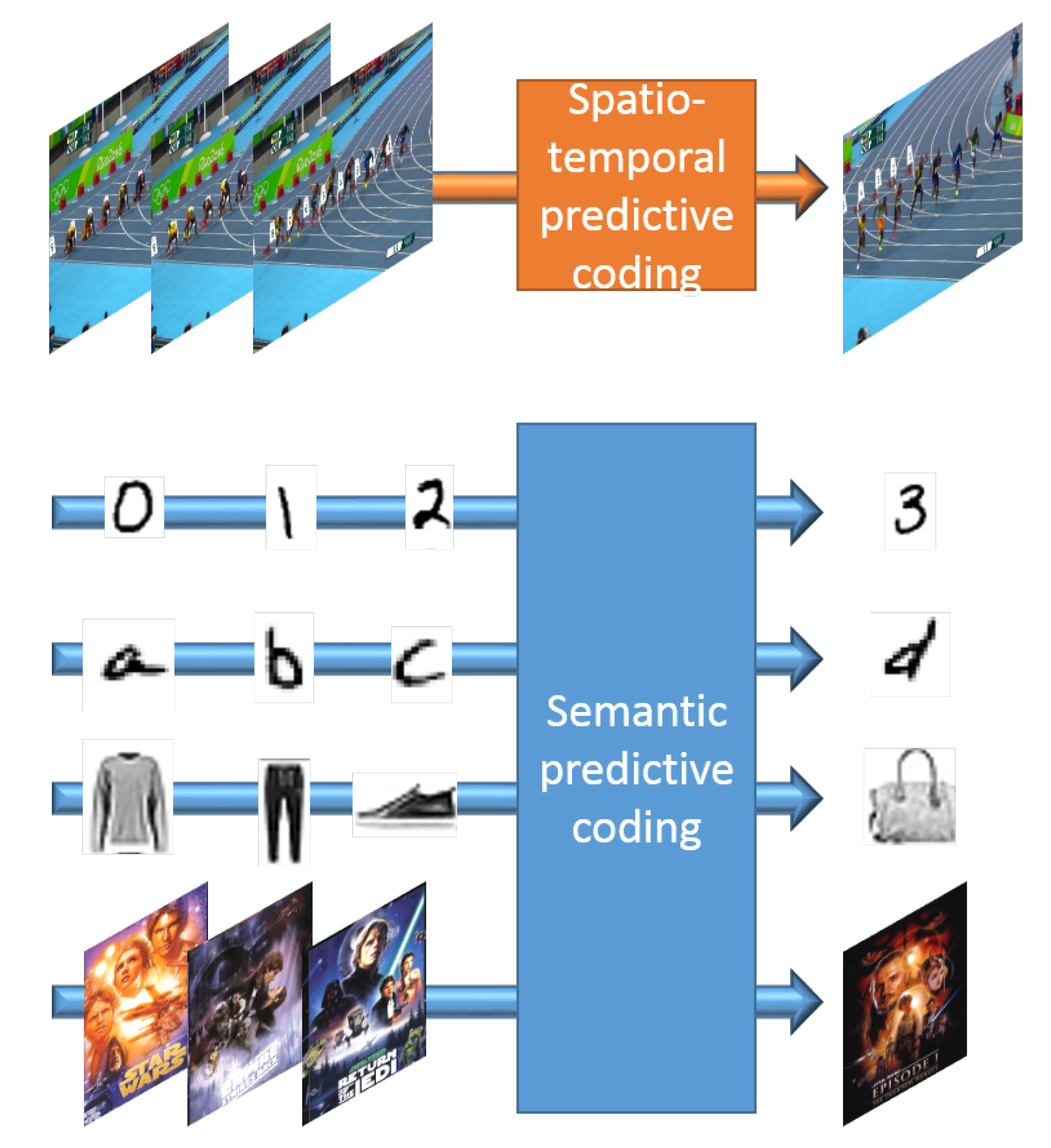
- The formulation of the semantic predictive coding paradigm as an extension of the traditional next-frame prediction paradigm.
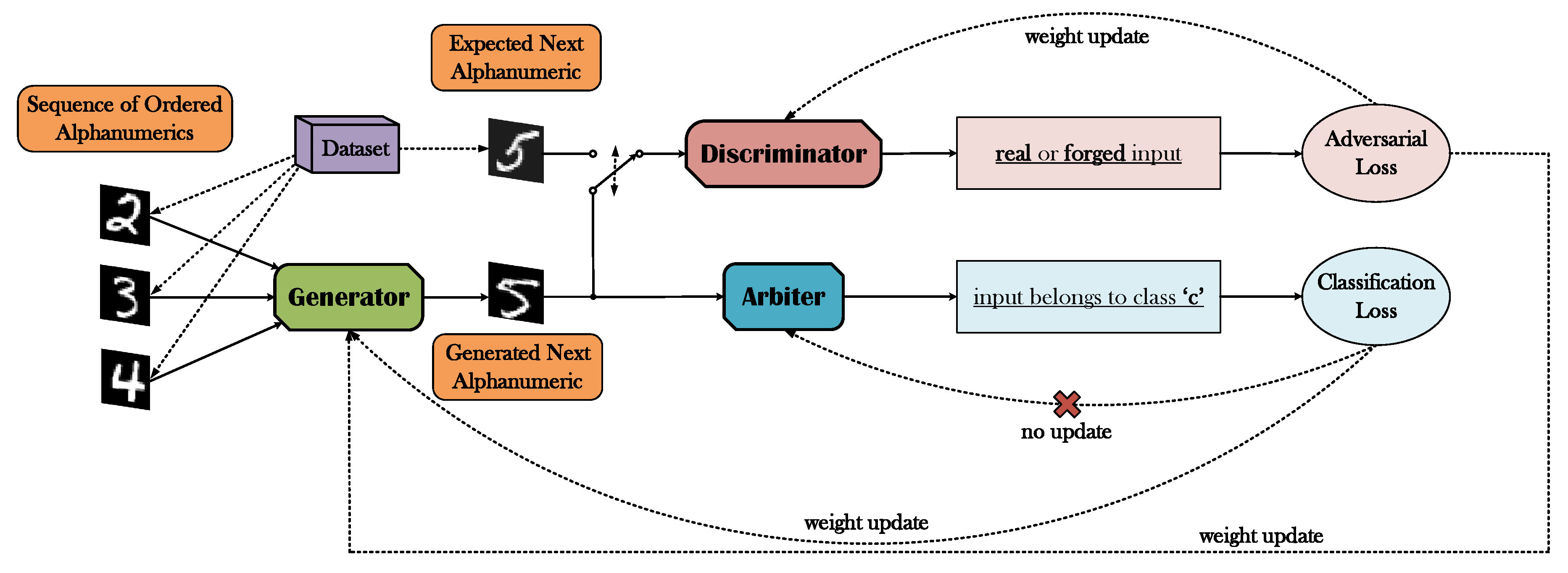
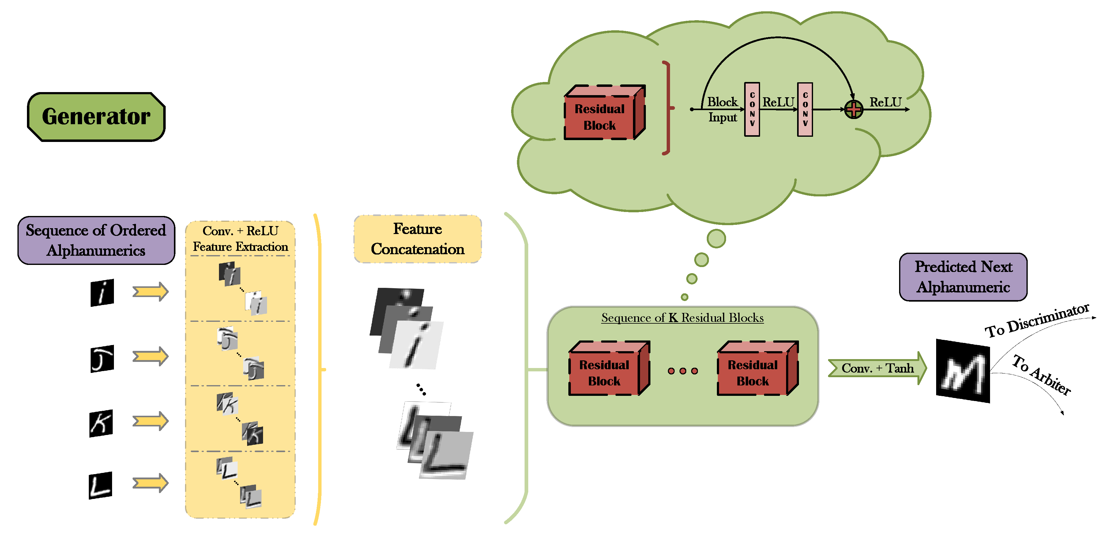
- The development of a novel generative DNN architecture termed Arbitrated Generative Adversarial Networks for addressing the semantic predictive coding.
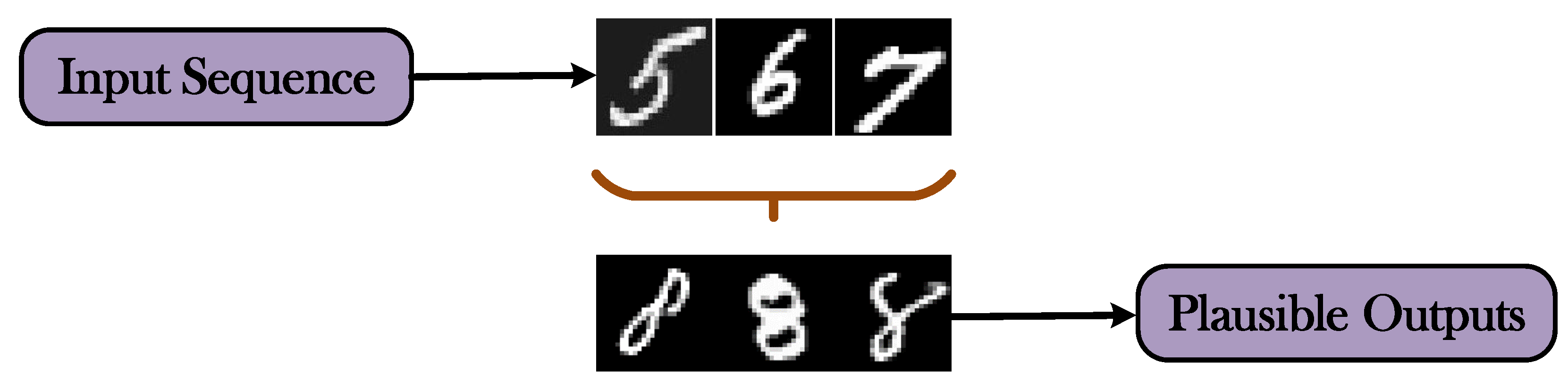
- The demonstration of the capabilities of the proposed framework on the visual prediction of alphanumeric sequences.
2. Related Work
3. Proposed Methodology
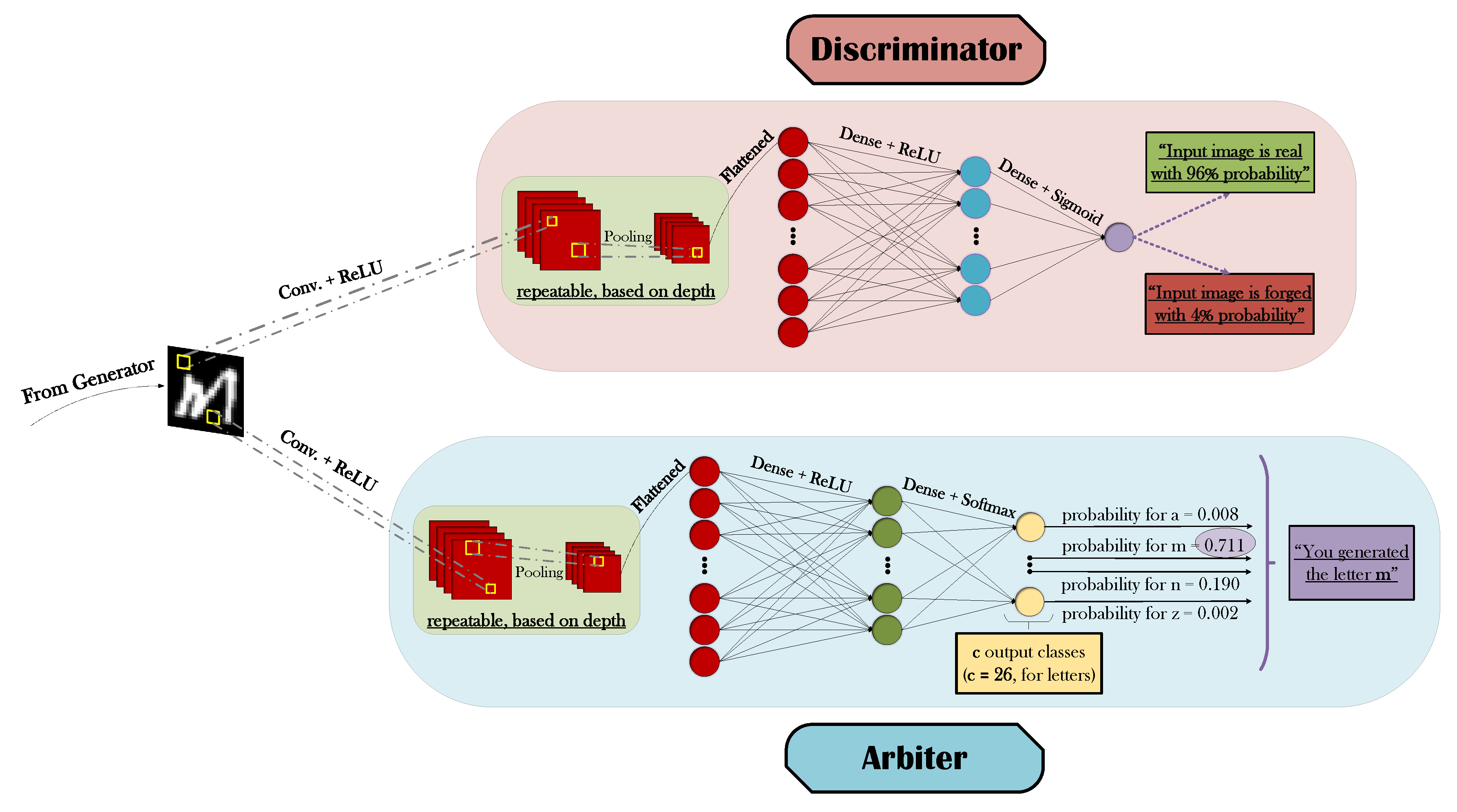
3.1. Generative Adversarial Networks
3.2. Arbiter Network
3.3. The A-GAN Framework
4. Experimental Analysis and Discussion
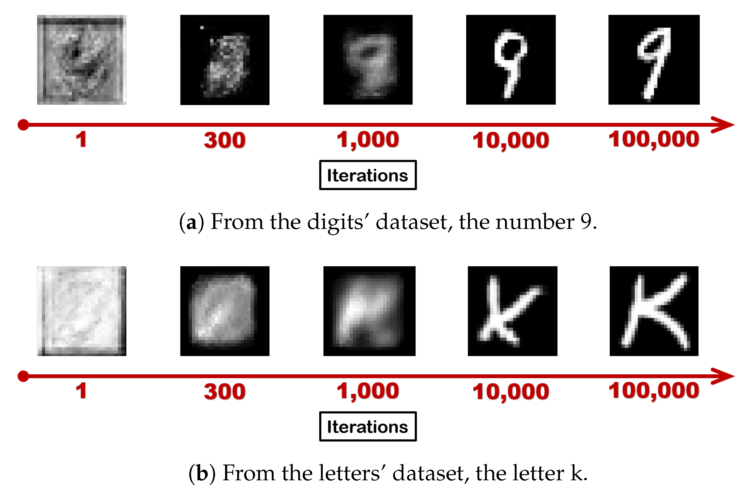
4.1. Dataset Manipulation
4.2. Experimental Setup
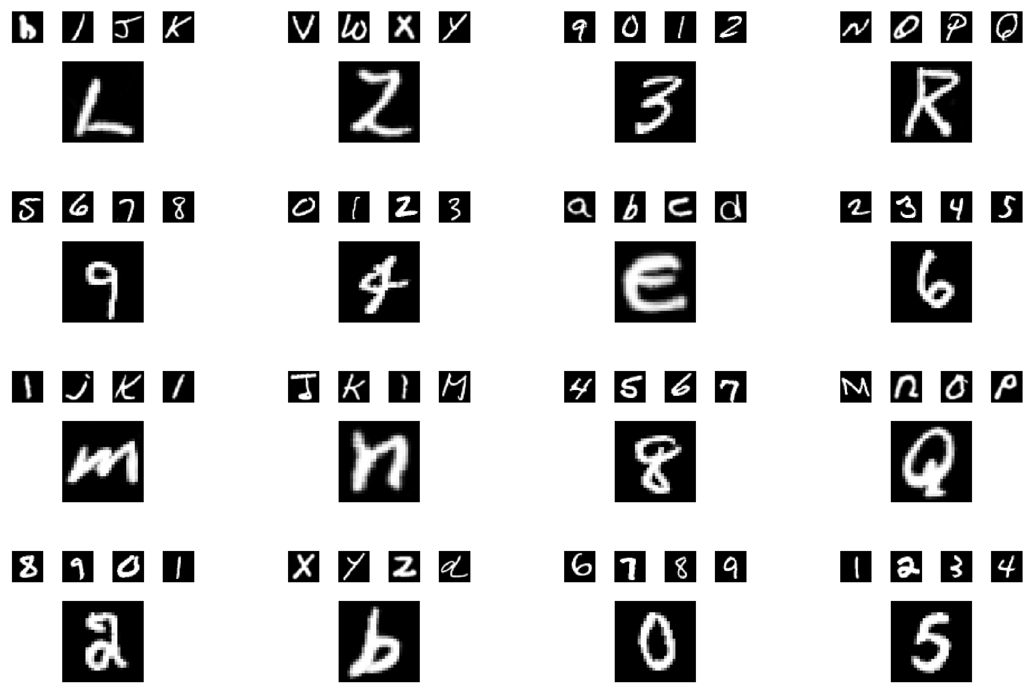
4.3. Qualitative and Quantitative Results
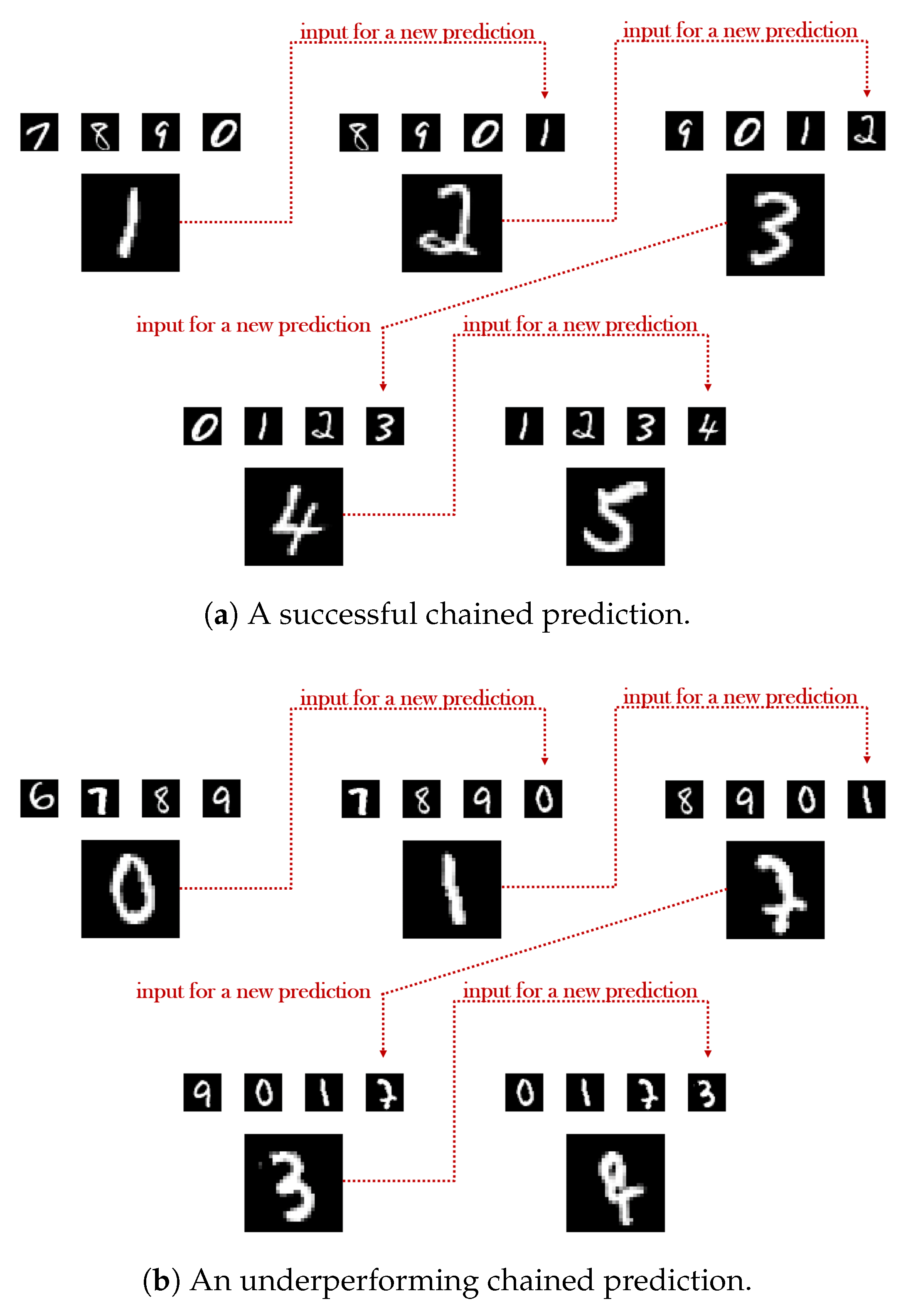
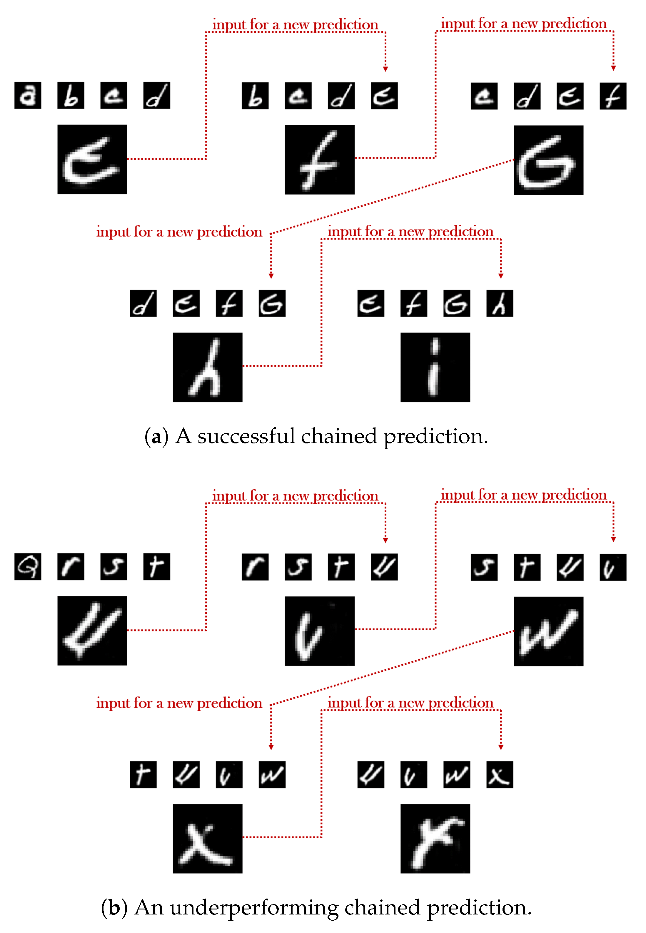
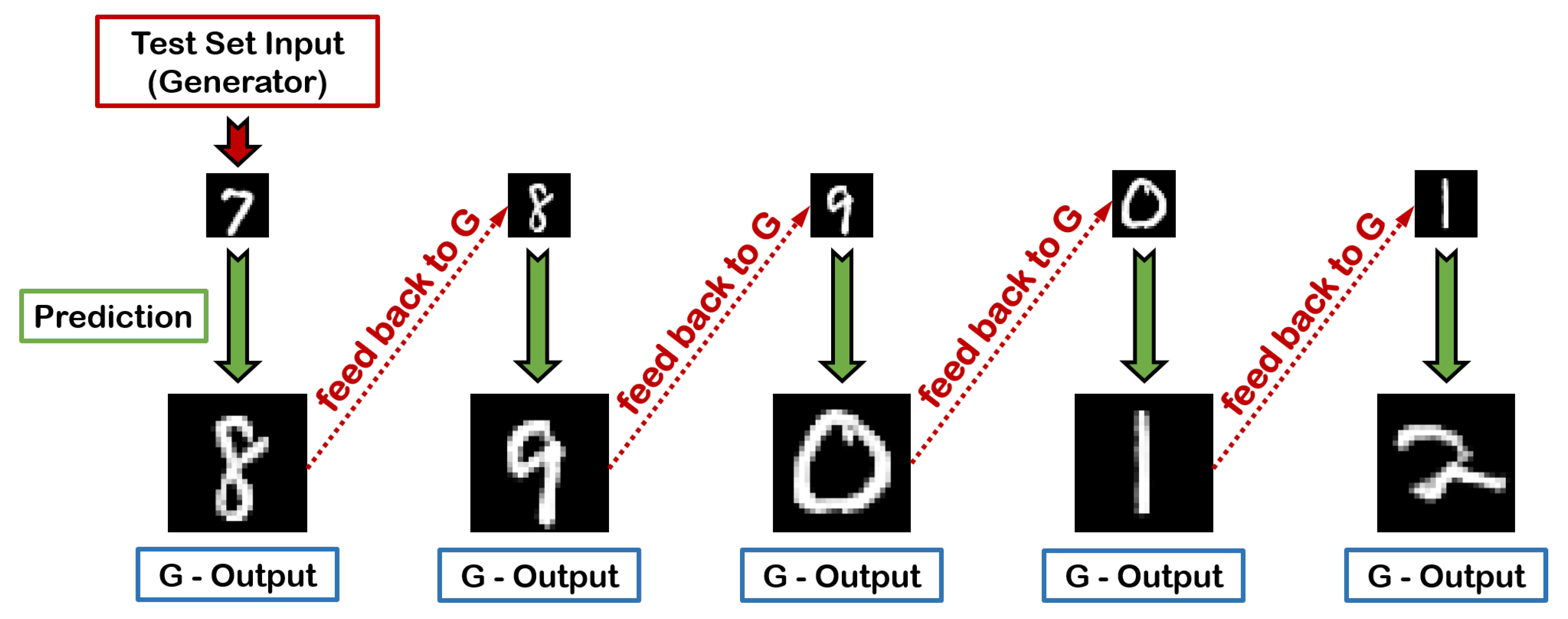
4.3.1. Chains of Consecutive Predictions
4.3.2. Impact of the Cardinality of the Input Sequence
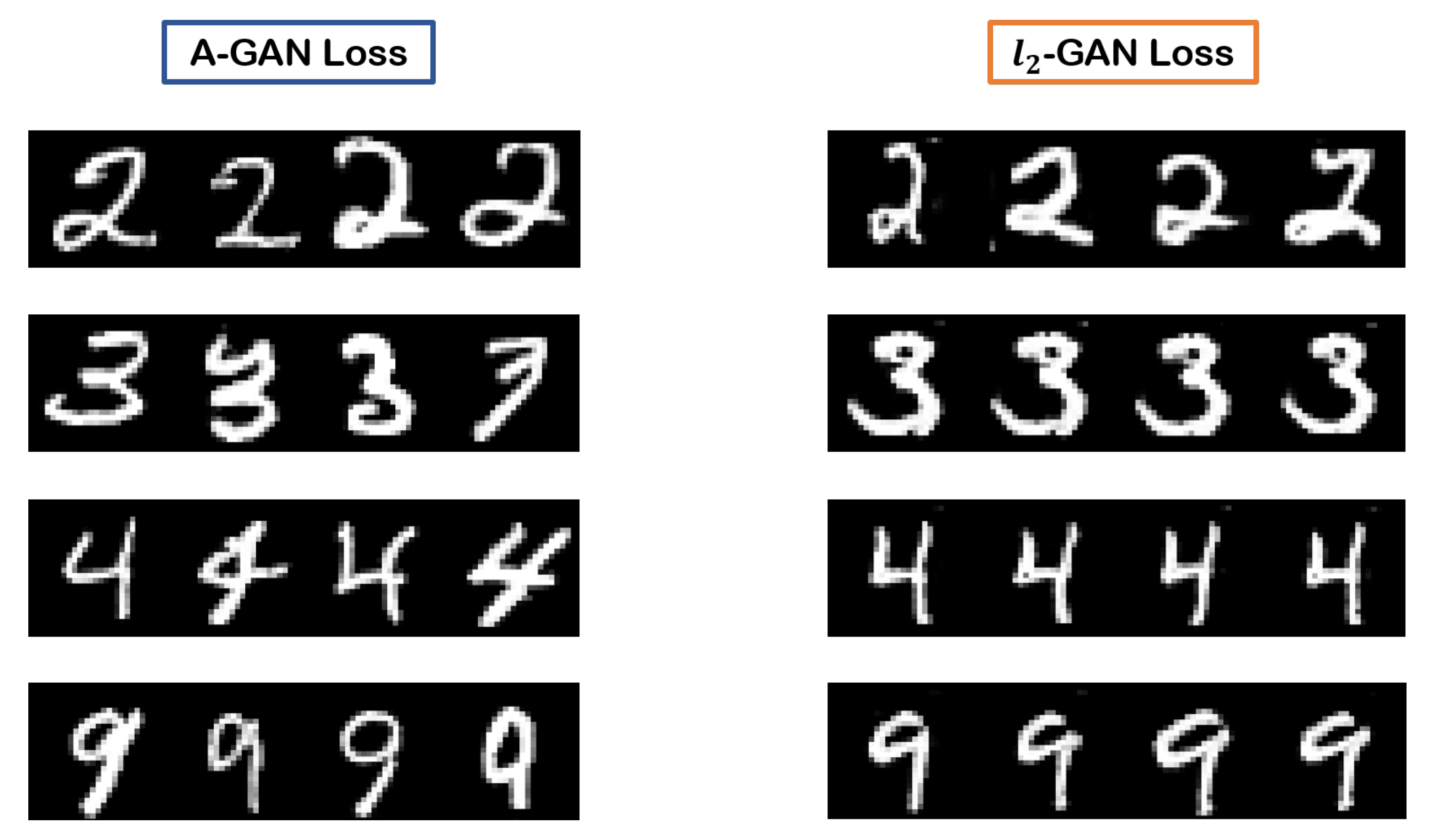
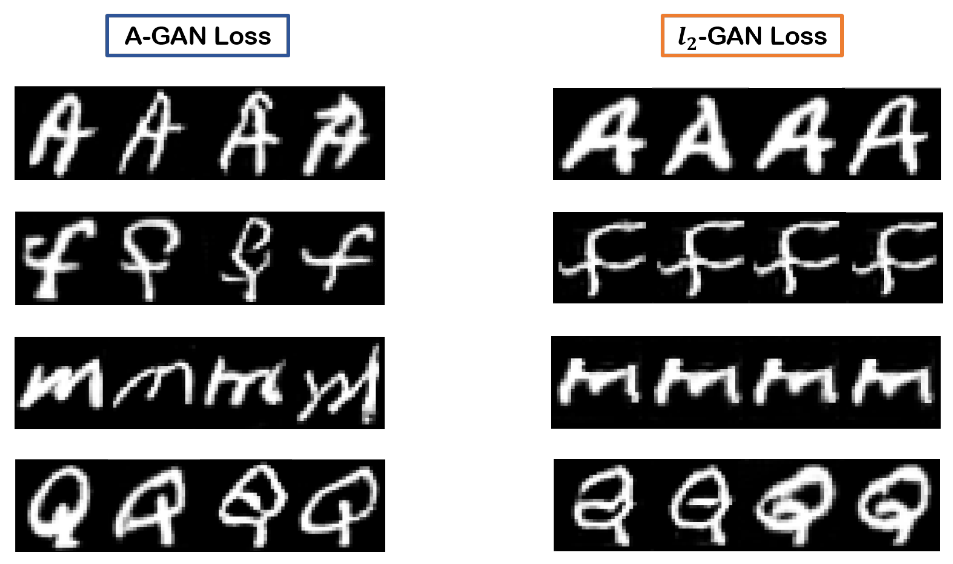
4.3.3. Arbiter’s Loss Versus Loss
5. Conclusions
Author Contributions
Funding
Acknowledgments
Conflicts of Interest
Abbreviations
| GAN(s) | Generative Adversarial Network(s) |
| AI | Artificial Intelligence |
| DNN(s) | Deep Neural Network(s) |
| A-GAN | Arbitrated Generative Adversarial Network |
| LSTM | Long Short Term Memory |
| ConvLSTM | Convolutional-LSTM |
| MSE | Mean Squared Error |
| CoGAN | Coupled Generative Adversarial Network |
| NIST | National Institute of Standards and Technology |
| MNIST | Modified NIST |
| EMNIST | Extended MNIST |
| VGG | Visual Geometry Group |
| ReLU | Rectified Linear Unit |
| (D)CNN(s) | (Deep) Convolutional Neural Network(s) |
| PSNR | Peak Signal to Noise Ratio |
| SSIM | Structural Similarity Index Measure |
References
- LeCun, Y.; Bengio, Y.; Hinton, G. Deep learning. Nature 2015, 521, 436–444. [Google Scholar] [CrossRef] [PubMed]
- Hochreiter, S.; Schmidhuber, J. Long short-term memory. Neural Comput. 1997, 9, 1735–1780. [Google Scholar] [CrossRef] [PubMed]
- Krizhevsky, A.; Sutskever, I.; Hinton, G.E. Imagenet classification with deep convolutional neural networks. In Proceedings of the Advances in Neural Information Processing Systems, Lake Tahoe, NV, USA, 3–6 December 2012; pp. 1097–1105. [Google Scholar]
- He, K.; Zhang, X.; Ren, S.; Sun, J. Deep residual learning for image recognition. In Proceedings of the IEEE Conference on Computer Vision and Pattern Recognition, Las Vegas, NV, USA, 27–30 June 2016; pp. 770–778. [Google Scholar]
- Rumelhart, D.E.; Hinton, G.E.; Williams, R.J. Learning Internal Representations by Error Propagation; Technical report; California University San Diego, La Jolla Institute for Cognitive Science: San Diego, CA, USA, 1985. [Google Scholar]
- Srinivasan, M.V.; Laughlin, S.B.; Dubs, A. Predictive coding: A fresh view of inhibition in the retina. Proc. R. Soc. Lond. Ser. B Biol. Sci. 1982, 216, 427–459. [Google Scholar]
- Ballard, D.H.; Hinton, G.E.; Sejnowski, T.J. Parallel visual computation. Nature 1983, 306, 21–26. [Google Scholar] [CrossRef] [PubMed]
- Rao, R.P.; Ballard, D.H. Predictive coding in the visual cortex: A functional interpretation of some extra-classical receptive-field effects. Nat. Neurosci. 1999, 2, 79–87. [Google Scholar] [CrossRef] [PubMed]
- Friston, K.; Kiebel, S. Predictive coding under the free-energy principle. Philos. Trans. R. Soc. B Biol. Sci. 2009, 364, 1211–1221. [Google Scholar] [CrossRef] [PubMed]
- Bastos, A.M.; Usrey, W.M.; Adams, R.A.; Mangun, G.R.; Fries, P.; Friston, K.J. Canonical microcircuits for predictive coding. Neuron 2012, 76, 695–711. [Google Scholar] [CrossRef] [PubMed]
- Friston, K. Does predictive coding have a future? Nat. Neurosci. 2018, 21, 1019–1021. [Google Scholar] [CrossRef] [PubMed]
- Zhou, Y.; Dong, H.; El Saddik, A. Deep Learning in Next-Frame Prediction: A Benchmark Review. IEEE Access 2020, 8, 69273–69283. [Google Scholar] [CrossRef]
- Goodfellow, I.; Pouget-Abadie, J.; Mirza, M.; Xu, B.; Warde-Farley, D.; Ozair, S.; Courville, A.; Bengio, Y. Generative adversarial nets. In Proceedings of the Advances in Neural Information Processing Systems, Montreal, QC, Canada, 8–13 December 2014; pp. 2672–2680. [Google Scholar]
- Vondrick, C.; Pirsiavash, H.; Torralba, A. Generating videos with scene dynamics. In Proceedings of the Advances in Neural Information Processing Systems, Barcelona, Spain, 5–10 September 2016; pp. 1–9. [Google Scholar]
- Tulyakov, S.; Liu, M.Y.; Yang, X.; Kautz, J. Mocogan: Decomposing motion and content for video generation. In Proceedings of the IEEE Conference on Computer Vision and Pattern Recognition, Salt Lake City, UT, USA, 18–23 June 2018; pp. 1526–1535. [Google Scholar]
- Wang, Y.; Jiang, L.; Yang, M.H.; Li, L.J.; Long, M.; Fei-Fei, L. Eidetic 3D lstm: A model for video prediction and beyond. In Proceedings of the International Conference on Learning Representations, New Orleans, LA, USA, 6–9 May 2019. [Google Scholar]
- Saito, M.; Matsumoto, E.; Saito, S. Temporal generative adversarial nets with singular value clipping. In Proceedings of the IEEE International Conference on Computer Vision, Venice, Italy, 22–27 October 2017; pp. 2830–2839. [Google Scholar]
- Rumelhart, D.E.; Hinton, G.E.; Williams, R.J. Learning representations by back-propagating errors. Nature 1986, 323, 533–536. [Google Scholar] [CrossRef]
- Michalski, V.; Memisevic, R.; Konda, K. Modeling deep temporal dependencies with recurrent grammar cells. In Proceedings of the Advances in Neural Information Processing Systems, Montreal, QC, Canada, 8–13 December 2014; pp. 1925–1933. [Google Scholar]
- Memisevic, R. Learning to relate images. IEEE Trans. Pattern Anal. Mach. Intell. 2013, 35, 1829–1846. [Google Scholar] [CrossRef] [PubMed]
- Srivastava, N.; Mansimov, E.; Salakhudinov, R. Unsupervised learning of video representations using lstms. In Proceedings of the 32nd International Conference on Machine Learning, Lille, France, 6–11 July 2015; pp. 843–852. [Google Scholar]
- Xingjian, S.; Chen, Z.; Wang, H.; Yeung, D.Y.; Wong, W.K.; Woo, W.c. Convolutional LSTM network: A machine learning approach for precipitation nowcasting. In Proceedings of the Advances in Neural Information Processing Systems, Montreal, QC, Canada, 7–12 December 2015; pp. 802–810. [Google Scholar]
- Lotter, W.; Kreiman, G.; Cox, D. Deep predictive coding networks for video prediction and unsupervised learning. In Proceedings of the International Conference on Learning Representations, Toulon, France, 24–26 April 2017; pp. 1–18. [Google Scholar]
- Rane, R.P.; Szügyi, E.; Saxena, V.; Ofner, A.; Stober, S. PredNet and Predictive Coding: A Critical Review. In Proceedings of the 2020 International Conference on Multimedia Retrieval, Dublin, Ireland, 8–11 June 2020; pp. 233–241. [Google Scholar]
- Villegas, R.; Yang, J.; Hong, S.; Lin, X.; Lee, H. Decomposing motion and content for natural video sequence prediction. In Proceedings of the International Conference on Learning Representations, Toulon, France, 24–26 April 2017; pp. 1–22. [Google Scholar]
- Wang, Y.; Long, M.; Wang, J.; Gao, Z.; Philip, S.Y. Predrnn: Recurrent neural networks for predictive learning using spatiotemporal lstms. In Proceedings of the Advances in Neural Information Processing Systems, Long Beach, CA, USA, 4–9 December 2017; pp. 879–888. [Google Scholar]
- Wang, Y.; Gao, Z.; Long, M.; Wang, J.; Yu, P.S. Predrnn++: Towards a resolution of the deep-in-time dilemma in spatiotemporal predictive learning. In Proceedings of the 35th International Conference on Machine Learning, Stockholm, Sweden, 10–15 July 2018; pp. 5123–5132. [Google Scholar]
- Mathieu, M.; Couprie, C.; LeCun, Y. Deep multi-scale video prediction beyond mean square error. In Proceedings of the International Conference on Learning Representations, ICLR 2016, San Juan, Puerto Rico, 2–4 May 2016; pp. 1–14. [Google Scholar]
- Radford, A.; Metz, L.; Chintala, S. Unsupervised representation learning with deep convolutional generative adversarial networks. In Proceedings of the International Conference on Learning Representations, ICLR 2016, San Juan, Puerto Rico, 2–4 May 2016; pp. 1–16. [Google Scholar]
- Lotter, W.; Kreiman, G.; Cox, D. Unsupervised learning of visual structure using predictive generative networks. In Proceedings of the International Conference on Learning Representations, ICLR 2016, San Juan, Puerto Rico, 2–4 May 2016. [Google Scholar]
- Zhou, Y.; Berg, T.L. Learning temporal transformations from time-lapse videos. In Proceedings of the European Conference on Computer Vision, ECCV 2016, Amsterdam, The Netherlands, 11–14 October 2016; pp. 262–277. [Google Scholar]
- Liang, X.; Lee, L.; Dai, W.; Xing, E.P. Dual motion GAN for future-flow embedded video prediction. In Proceedings of the IEEE International Conference on Computer Vision, Venice, Italy, 22–29 October 2017; pp. 1744–1752. [Google Scholar]
- Lu, C.; Hirsch, M.; Scholkopf, B. Flexible spatio-temporal networks for video prediction. In Proceedings of the IEEE Conference on Computer Vision and Pattern Recognition, Honolulu, HI, USA, 21–26 July 2017; pp. 6523–6531. [Google Scholar]
- Vondrick, C.; Torralba, A. Generating the future with adversarial transformers. In Proceedings of the IEEE Conference on Computer Vision and Pattern Recognition, Honolulu, HI, USA, 21–26 July 2017; pp. 1020–1028. [Google Scholar]
- Bhattacharjee, P.; Das, S. Temporal coherency based criteria for predicting video frames using deep multi-stage generative adversarial networks. In Proceedings of the Advances in Neural Information Processing Systems, Long Beach, CA, USA, 4–9 December 2017; pp. 4268–4277. [Google Scholar]
- Wichers, N.; Villegas, R.; Erhan, D.; Lee, H. Hierarchical long-term video prediction without supervision. In Proceedings of the 35th International Conference on Machine Learning, ICML 2018, Stockholm, Sweden, 10–15 July 2018. [Google Scholar]
- Kwon, Y.H.; Park, M.G. Predicting future frames using retrospective cycle gan. In Proceedings of the IEEE Conference on Computer Vision and Pattern Recognition, Long Beach, CA, USA, 15–21 June 2019; pp. 1811–1820. [Google Scholar]
- Aigner, S.; Körner, M. FUTUREGAN: Anricipating the future frames of video sequences using spatio-temporal 3D convolutions in progressively growing gans. ISPRS Int. Arch. Photogramm. Remote Sens. Spat. Inf. Sci. 2019, XLII-2/W16, 3–11. [Google Scholar] [CrossRef]
- Ledig, C.; Theis, L.; Huszár, F.; Caballero, J.; Cunningham, A.; Acosta, A.; Aitken, A.; Tejani, A.; Totz, J.; Wang, Z.; et al. Photo-realistic single image super-resolution using a generative adversarial network. In Proceedings of the Proceedings of the IEEE Conference on Computer Vision and Pattern Recognition, Honolulu, HI, USA, 21–26 July 2017; pp. 4681–4690. [Google Scholar]
- Lucas, A.; Lopez-Tapia, S.; Molina, R.; Katsaggelos, A.K. Generative adversarial networks and perceptual losses for video super-resolution. IEEE Trans. Image Process. 2019, 28, 3312–3327. [Google Scholar] [CrossRef] [PubMed]
- Reed, S.; Akata, Z.; Yan, X.; Logeswaran, L.; Schiele, B.; Lee, H. Generative adversarial text to image synthesis. In Proceedings of the 33rd International Conference on Machine Learning, ICML, New York, NY, USA, 20–22 June 2016. [Google Scholar]
- Zhang, H.; Xu, T.; Li, H.; Zhang, S.; Wang, X.; Huang, X.; Metaxas, D.N. Stackgan: Text to photo-realistic image synthesis with stacked generative adversarial networks. In Proceedings of the IEEE International Conference on Computer Vision, Venice, Italy, 22–29 October 2017; pp. 5907–5915. [Google Scholar]
- Liu, X.; Meng, G.; Xiang, S.; Pan, C. Semantic image synthesis via conditional cycle-generative adversarial networks. In Proceedings of the 2018 24th International Conference on Pattern Recognition (ICPR), IEEE, Beijing, China, 20–24 August 2018; pp. 988–993. [Google Scholar]
- Pathak, D.; Krahenbuhl, P.; Donahue, J.; Darrell, T.; Efros, A.A. Context encoders: Feature learning by inpainting. In Proceedings of the IEEE Conference on Computer Vision and Pattern Recognition, Las Vegas, NV, USA, 27–30 June 2016; pp. 2536–2544. [Google Scholar]
- Denton, E.L.; Chintala, S.; Fergus, R. Deep generative image models using a laplacian pyramid of adversarial networks. In Proceedings of the Advances in Neural Information Processing Systems, Montreal, QC, Canada, 7–12 December 2015; pp. 1486–1494. [Google Scholar]
- Li, C.; Wand, M. Precomputed real-time texture synthesis with markovian generative adversarial networks. In Proceedings of the European Conference on Computer Vision, Amsterdam, The Netherlands, 11–14 October 2016; pp. 702–716. [Google Scholar]
- Larsen, A.B.L.; Sønderby, S.K.; Larochelle, H.; Winther, O. Autoencoding beyond pixels using a learned similarity metric. In Proceedings of the 33rd International Conference on Machine Learning, New York, NY, USA, 20–22 June 2016; Volume 48, pp. 1558–1566. [Google Scholar]
- Karras, T.; Laine, S.; Aila, T. A style-based generator architecture for generative adversarial networks. In Proceedings of the IEEE Conference on Computer Vision and Pattern Recognition, Long Beach, CA, USA, 15–20 June 2019; pp. 4401–4410. [Google Scholar]
- Mirza, M.; Osindero, S. Conditional generative adversarial nets. arXiv 2014, arXiv:1411.1784. [Google Scholar]
- Arjovsky, M.; Chintala, S.; Bottou, L. Wasserstein Generative Adversarial Networks. In Proceedings of the 34th International Conference on Machine Learning, Sydney, NSW, Australia, 6–11 August 2017; Volume 70, pp. 214–223. [Google Scholar]
- Dobrushin, R.L. Prescribing a system of random variables by conditional distributions. Theory Probab. Appl. 1970, 15, 458–486. [Google Scholar] [CrossRef]
- Liu, M.Y.; Tuzel, O. Coupled generative adversarial networks. In Proceedings of the Advances in Neural Information Processing Systems, Barcelona, Spain, 5–10 December 2016; pp. 469–477. [Google Scholar]
- LeCun, Y.; Cortes, C.; Burges, C. MNIST handwritten digit database. ATT Labs 2010, 2. Available online: http://yann.lecun.com/exdb/mnist (accessed on 18 January 2020).
- Cohen, G.; Afshar, S.; Tapson, J.; Schaik, A.V. EMNIST: Extending MNIST to handwritten letters. In Proceedings of the 2017 International Joint Conference on Neural Networks (IJCNN), Anchorage, AK, USA, 14–19 May 2017. [Google Scholar] [CrossRef]
- Nair, V.; Hinton, G.E. Rectified linear units improve restricted boltzmann machines. In Proceedings of the 27th International Conference on Machine Learning, ICML, Haifa, Israel, 21–24 June 2010. [Google Scholar]
- Xu, B.; Wang, N.; Chen, T.; Li, M. Empirical evaluation of rectified activations in convolutional network. arXiv 2015, arXiv:1505.00853. [Google Scholar]
- LeCun, Y.; Boser, B.; Denker, J.S.; Henderson, D.; Howard, R.E.; Hubbard, W.; Jackel, L.D. Backpropagation applied to handwritten zip code recognition. Neural Comput. 1989, 1, 541–551. [Google Scholar] [CrossRef]
- Srivastava, N.; Hinton, G.; Krizhevsky, A.; Sutskever, I.; Salakhutdinov, R. Dropout: A simple way to prevent neural networks from overfitting. J. Mach. Learn. Res. 2014, 15, 1929–1958. [Google Scholar]
- Ioffe, S.; Szegedy, C. Batch Normalization: Accelerating Deep Network Training by Reducing Internal Covariate Shift. In Proceedings of the 32nd International Conference on Machine Learning, Lille, France, 6–11 July 2015; Volume 37, pp. 448–456. [Google Scholar]
- Wang, Z.; Bovik, A.C.; Sheikh, H.R.; Simoncelli, E.P. Image quality assessment: From error visibility to structural similarity. IEEE Trans. Image Process. 2004, 13, 600–612. [Google Scholar] [CrossRef]


| 1st in Chain | 2nd in Chain | 3rd in Chain | 4th in Chain | 5th in Chain | |
|---|---|---|---|---|---|
| Potent Model | 99.50% | 99.34% | 99.36% | 99.06% | 98.74% |
| Underperforming Model | 97.52% | 92.22% | 83.74% | 73.46% | 61.01% |
| 1st in Chain | 2nd in Chain | 3rd in Chain | 4th in Chain | 5th in Chain | |
|---|---|---|---|---|---|
| Potent Model | 95.84% | 94.88% | 93.08% | 92.36% | 91.28% |
| Underperforming Model | 88.18% | 85.90% | 80.08% | 72.29% | 60.71% |
| 1st in Chain | 2nd in Chain | 3rd in Chain | 4th in Chain | 5th in Chain | |
|---|---|---|---|---|---|
| 4 input frames | 99.50% | 99.34% | 99.36% | 99.06% | 98.74% |
| 3 input frames | 99.06% | 98.68% | 98.04% | 97.90% | 96.18% |
| 2 input frames | 98.08% | 97.46% | 96.86% | 95.46% | 92.92% |
| 1 input frame | 97.44% | 96.20% | 95.08% | 93.16% | 90.34% |
| 1st in Chain | 2nd in Chain | 3rd in Chain | 4th in Chain | 5th in Chain | |
|---|---|---|---|---|---|
| 4 input frames | 95.84% | 94.88% | 93.08% | 92.36% | 91.28% |
| 3 input frames | 94.54% | 92.82% | 91.45% | 89.72% | 87.13% |
| 2 input frames | 91.10% | 87.40% | 82.20% | 79.24% | 73.68% |
| 1 input frame | 85.50% | 76.12% | 67.24% | 60.62% | 54.02% |
| 1st in Chain | 2nd in Chain | 3rd in Chain | 4th in Chain | 5th in Chain | |
|---|---|---|---|---|---|
| A-GAN best case—digits | 99.50% | 99.34% | 99.36% | 99.06% | 98.74% |
| -GAN best case—digits | 99.26% | 99.34% | 99.20% | 99.04% | 98.71% |
| A-GAN best case—letters | 95.84% | 94.88% | 93.08% | 92.36% | 91.28% |
| -GAN best case—letters | 83.23% | 82.58% | 82.16% | 81.24% | 80.84% |
© 2020 by the authors. Licensee MDPI, Basel, Switzerland. This article is an open access article distributed under the terms and conditions of the Creative Commons Attribution (CC BY) license (http://creativecommons.org/licenses/by/4.0/).
Share and Cite
Stivaktakis, R.; Tsagkatakis, G.; Tsakalides, P. Semantic Predictive Coding with Arbitrated Generative Adversarial Networks. Mach. Learn. Knowl. Extr. 2020, 2, 307-326. https://doi.org/10.3390/make2030017
Stivaktakis R, Tsagkatakis G, Tsakalides P. Semantic Predictive Coding with Arbitrated Generative Adversarial Networks. Machine Learning and Knowledge Extraction. 2020; 2(3):307-326. https://doi.org/10.3390/make2030017
Chicago/Turabian StyleStivaktakis, Radamanthys, Grigorios Tsagkatakis, and Panagiotis Tsakalides. 2020. "Semantic Predictive Coding with Arbitrated Generative Adversarial Networks" Machine Learning and Knowledge Extraction 2, no. 3: 307-326. https://doi.org/10.3390/make2030017
APA StyleStivaktakis, R., Tsagkatakis, G., & Tsakalides, P. (2020). Semantic Predictive Coding with Arbitrated Generative Adversarial Networks. Machine Learning and Knowledge Extraction, 2(3), 307-326. https://doi.org/10.3390/make2030017