Article

Multi-Label Classification with Optimal Thresholding for Multi-Composition Spectroscopic Analysis

Department of Electrical and Computer Engineering, University of Victoria, EOW 448, 3800 Finnerty Rd., Victoria, BC V8P 5C2, Canada
*
Author to whom correspondence should be addressed.
Mach. Learn. Knowl. Extr. 2019, 1(4), 1084-1099; https://doi.org/10.3390/make1040061
Submission received: 25 September 2019 / Revised: 30 October 2019 / Accepted: 1 November 2019 / Published: 5 November 2019
(This article belongs to the Section Network)

Abstract

:
In this paper, we implement multi-label neural networks with optimal thresholding to identify gas species among a multiple gas mixture in a cluttered environment. Using infrared absorption spectroscopy and tested on synthesized spectral datasets, our approach outperforms conventional binary relevance-partial least squares discriminant analysis when the signal-to-noise ratio and training sample size are sufficient.

Graphical Abstract

1. Introduction

Spectroscopic analysis sees multiple applications in physics, chemistry, bioinformatics, geophysics, astronomy, etc. It has been widely used for detecting mineral samples [1], gas emission [2] and food volatiles [3]. Multivariate regression algorithms such as principal component regression [4] and partial least squares (PLS) [5] are fundamental and popular tools that have been successfully applied to spectroscopic analysis. Non-linear methods, such as support vector machine [6], genetic programming [7] and artificial neural networks (ANN) [1], are also adopted to increase prediction accuracy. These algorithms focus on either regression or single-label classification problems. Using multi-label classification to identify multiple chemical components from the spectrum is under explored. Unlike multi-classification counterparts that utilize multiple values of a single label to identify different spectroscopic components, multi-label methods adopt two or more output labels, one for each individual component. Consequently, relations between labels in multi-label tasks can be either independent or correlated.
The development of multi-label classification dates back to the 1990s when binary relevance (BR) [8] and the boosting method [9] were introduced to solve text categorization problems. A significant amount of research was done after that, and multi-label learning has been prosperous in areas such as natural language processing and image recognition [10,11,12,13,14,15,16]. Most of the multi-label classification algorithms fall into two basic categories: problem transformation and algorithm adaption. Problem transformation algorithms transform a multi-label problem into one or more single-label problems. After the transformation, existing single-label classifiers can be implemented to make predictions, and the combined outputs will be transformed back into multi-label representations. One of the simplest problem transformation methods is BR. It transforms a multi-label problem by splitting it into one binary problem for each label [17,18]. Under the assumption of label independence, it ignores the correlations between labels. If such an assumption fails, the label powerset (LP) and classifier chains (CC) are known transformation alternatives, where LP maps one subset of original labels into one class of the new single label [19] and CC passes label correlation information along a chain of classifiers [20]. For large label spaces where LP maps too many new labels to classify, label embedding techniques [21,22,23] divide the label space into subspaces and exploit the dependencies between them. In contrast, algorithm adaption methods modify existing single-label classifiers to produce multi-label outputs. For instance, the extensions of decision tree [24], AdaBoost [9], and k-nearest neighbours (KNN) [25,26] are all designed to deal with multi-label classification problems. The restricted Boltzmann machine [27], feedforward neural networks (FNN) [28,29], convolutional neural networks (CNN) [30,31], and recurrent neural networks (RNN) [32] are employed to characterize label dependency in image processing or to find feature representations in text classification. Those adaptive methods can identify multiple labels simultaneously and efficiently without being repeatedly trained for sets of labels or chains of classifiers.
Our application of multi-label learning for spectroscopic analysis adopts FNN with optimal thresholding (FNN-OT), which is an adaptive FNN model inspired by [28,29]. It will be compared with other problem transformation and algorithm adaption models that are extended from PLS and FNN. In this article, we will train all the models with simulated spectroscopic datasets and compare their results. It will be shown that for most evaluation metrics, the adaptive FNN model has the best performance.

2. Dataset

To synthesize the datasets, firstly, single gas molecule mid-infrared absorption cross-section spectra of C 2 H 6 , C H 4 , C O , H 2 O , H B r , H C l , H F , N 2 O , and N O measured at 296 K were selected from the high-resolution transmission molecular absorption (HITRAN) database [33] and are displayed in Figure 1a. These nine gases were selected to test the validity of our machine learning algorithm in many-gas environments. The gas spectra were down sampled to 1000 points equally spaced between 1 micrometer ( μ m) and 7 μ m wavelengths. Secondly, the gas concentrations were randomly generated from a uniformly distributed probability density function such that the concentration of each gas was uniformly distributed between 0 and 10 micromolar ( μ M). Thirdly, in real scenarios, gases could be partially correlated. To verify our model under partially correlated components, we introduced highly positive correlation between some gases so that their concentrations retained a pre-set correlation. The generation of uniformly distributed random variables with the target correlation matrix will be discussed in Appendix A. Further, in order to test the validity of our classification model, we modified the concentration matrix such that each gas only appeared in 50% of the gas mixture samples. Using the concentration matrix, the absorption spectrum of each gas mixture was synthesized using the Beer–Lambert law, assuming that the gas mixture was contained in a 10 cm long sensing region. Lastly, artificial Gaussian noises with a pre-set signal-to-noise ratio (SNR) were added to the constant light intensity across each wavelength point in order to obtain a closer-to-reality spectrum and evaluate our model’s accuracy in different noise environments. In our simulation, the math expression of the transmitted light intensity I ( λ ) as a function of wavelength λ , given a light source with constant intensity I 0 and a Gaussian noise δ , can be written as:
I ( λ ) = I 0 ( 1 + δ ) e x p { i N i b σ i ( λ ) }
where N i is the molecule concentration of the i-th gas in units of the number of particles per m 3 . b is the length of the sensing regime, and σ i ( λ ) is the corresponding absorption cross-section obtained from HITRAN. δ = N ( 0 , σ δ 2 ) is a Gaussian random variable with zero mean and a variance of σ δ 2 such that the signal-to-noise ratio (SNR) of the light source in units of dB can be expressed as SNR ( dB ) = 10 log 10 σ δ . As an illustration, at SNR = 30 dB , a sample gas mixture spectrum with each gas concentration of 7.024 μ M, 0 μ M, 8.908 μ M, 9.816 μ M, 7.793 μ M, 4.575 μ M, 0 μ M, 0 μ M and 1.987 μ M, respectively, is plotted in Figure 1b.
In this article, we used 12 datasets, and each had a pre-set SNR of 0 dB , 10 dB , 20 dB , 30 dB , 40 dB and 50 dB . For each SNR, we generated two datasets respectively to represent uncorrelated and highly correlated cases. In uncorrelated cases, nine gas labels were mutually independent. In highly correlated cases, nine gases were evenly divided into three subsets. Gas labels within the same subset were highly correlated, and labels from different subsets were independent (Appendix A).

3. Algorithm

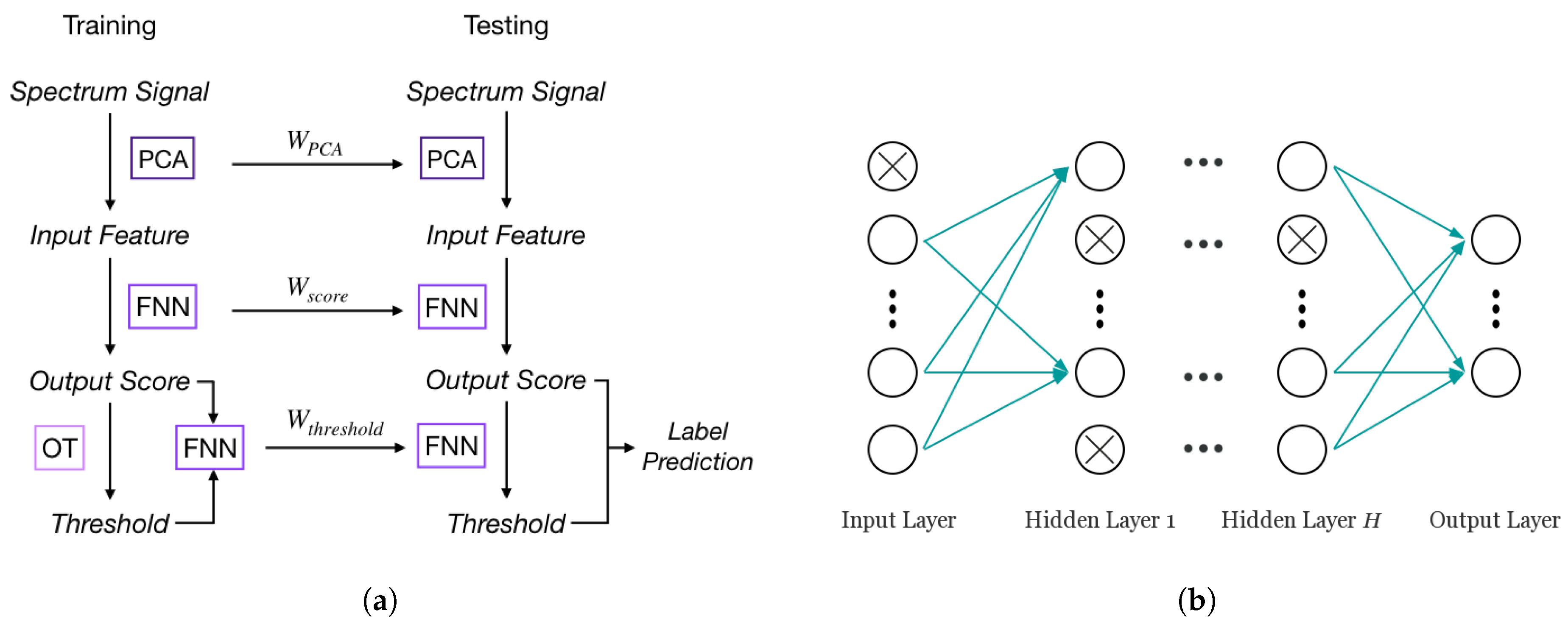
In single-label learning, a typical approach to classify an instance is to rank the probabilities (or scores) of all classes and choose the class with the highest probability as the prediction. For multi-label problems, the same ranking system can be used to compute scores for all labels instead, then a threshold will be determined to assign all labels whose scores are higher than the threshold to the sample. This label score-label prediction framework is the foundation of adapting NN for multi-label learning. In the FNN-OT model, scores of all labels need to be calculated for ranking purposes, and a threshold decision model will be employed to assign a set of labels to the sample in the label prediction step. The whole process of FNN-OT is shown in Figure 2a. Spectrum signals are firstly pre-processed by principal component analysis (PCA). The output principal components are the input features of an FNN model, which produces one output score for each gas. Output scores will be the input of a following optimal thresholding (OT). For every sample in the training set, its threshold will be determined by OT (details in Section 3.3). Then, the output scores and thresholds are the input and output variables of a new FNN model, which will be used to calculate thresholds for testing samples.

3.1. Feedforward Neural Networks

FNN has outstanding performance with large scale datasets [29]. As shown in Figure 2b, a typical FNN is formed by an input layer, an output layer and one or more hidden layers in-between. Each layer has a number of active neurons (circles without crosses in Figure 2b) that use the neuron outputs from previous layer as input and produce output to the neurons in the next layer. Previous research [29] showed that the single hidden layer model performs well on large scale text datasets. Furthermore, a preliminary test for the number of hidden layers was conducted on FNN without dropout. The results shown in Figure 1c indicate that FNN with only one hidden layer inside has the lowest Hamming loss, while the loss is higher in the cases of multiple hidden layers due to overfitting. Therefore, in our case of multi-label learning, a simple one hidden layer FNN model can achieve a state-of-the-art result with great computational efficiency. To get output score s based on input feature set x , our FNN can be written as [34]:
h = f h ( W ( 1 ) P ( 1 ) x + b ( 1 ) ) s = f s ( W ( 2 ) P ( 2 ) h + b ( 2 ) )
where h is a hidden layer that lies between the input and output layer, f h is the rectified linear units (ReLU) activation function in the hidden layer, f s is the sigmoid function for the output layer, and W ( 1 ) , W ( 2 ) , b ( 1 ) and b ( 2 ) are the parameters that need to be trained from data. In our model, the loss function f L ( s , y ) is defined as the cross-entropy of label score s and classification target y , which can be expressed as:
f L ( s , y ) = i = 1 L y i log ( s i ) + ( 1 y i ) log ( 1 s i )
where L is the number of labels.
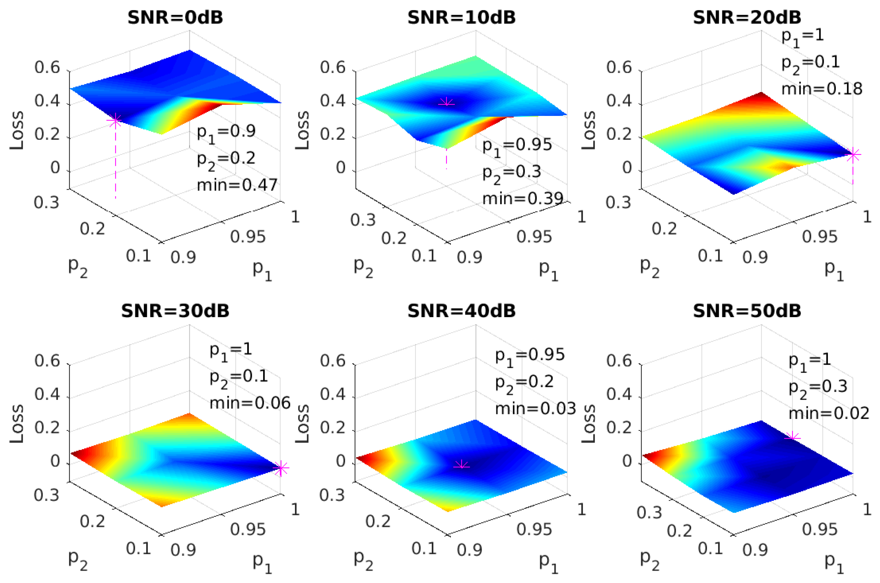
In our model, we adopted dropout to mitigate overfitting [34]. Dropout is a widely used method for preventing overfitting problems in neural networks. It randomly drops out a percentage of neurons in training, and the weights of remaining neurons will be trained by back-propagation [34]. Retention probability p = ( p 1 , p 2 ) is the hyperparameter of dropout that will be tuned for our model. p 1 and p 2 are the probabilities of retaining units in the input and the hidden layer of the neural network model. Retention probabilities set for the FNN-OT model are the ones that result in minimum losses. The dropout is activated by two diagonal matrices of Bernoulli random variables P ( 1 ) and P ( 2 ) with parameters p 1 and p 2 . Both parameters are retention probabilities of the input and hidden layer for dropout.

3.2. Principal Component Analysis

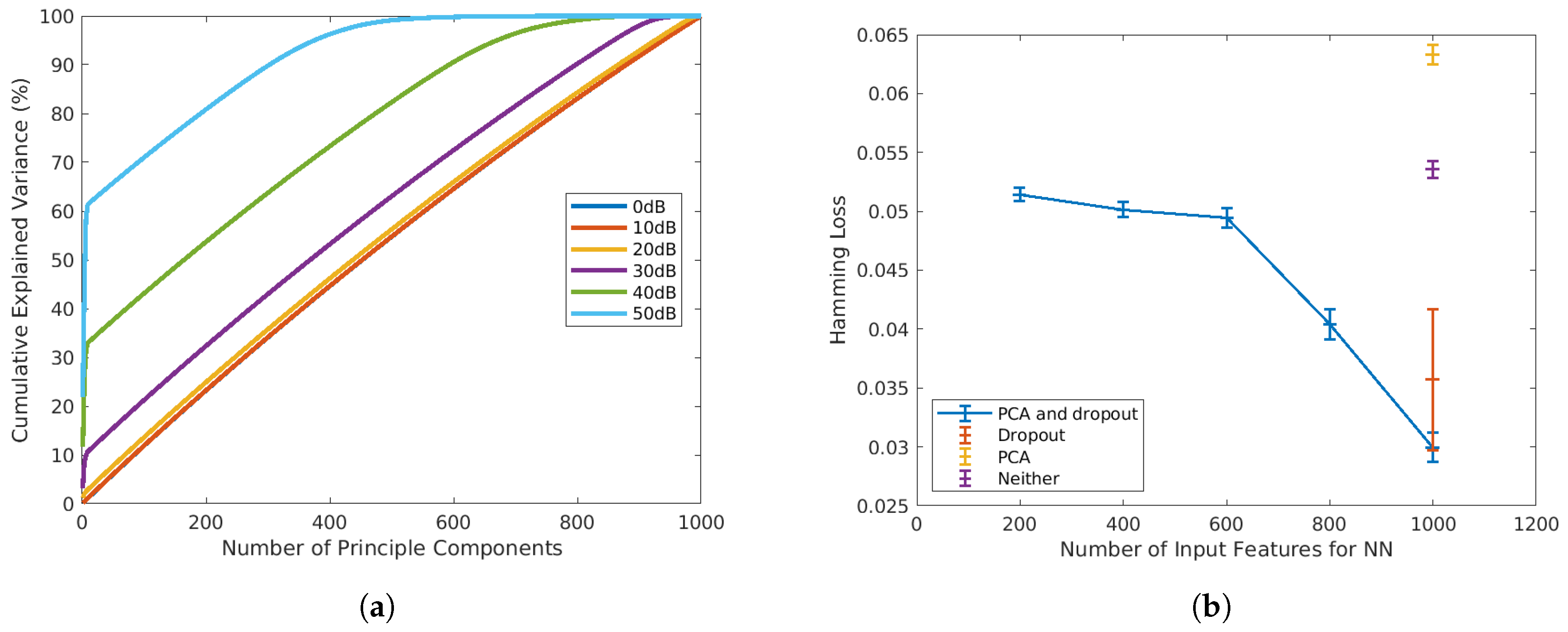
In both training and testing, the 1000-point absorbance spectra will be pre-processed with principal component analysis (PCA), and the principal components will be the input of the FNN model (x). PCA is a commonly used pre-processing method for spectroscopic datasets. It is conventionally employed to reduce the feature dimension by transferring original input variables into a smaller set of uncorrelated principal components (PC) that preserves the highest explained variance [35]. As shown in Figure 3a, at high SNR, PCA is an efficient technique for dimension reduction, as only a small number of PCs is sufficient to preserve most of the variances. However, when the SNR drops to below 30 dB, the variance of the original data is almost evenly projected into PCs. Under such circumstances, PCA will not be efficient for dimension reduction. Therefore, in a preliminary 10-fold test on the SNR = 40 dB dataset, Hamming loss has higher means when the number of PCs is less than the number of original inputs (blue line in Figure 3b). However, as shown in the same plot, when PCA is adopted in conjunction with dropout (blue markers), the Hamming loss is significantly reduced compared to the models that only adopt PCA (yellow markers), or dropout (red marker) or neither of them (purple marker). Therefore, in this article, we adopt PCA and dropout for all SNRs, not only for dimension reduction, but also for Hamming loss reductions.

3.3. Optimal Thresholding

Once we obtain the output score s for a specific instance, we need to find a threshold t i to convert the i-th label score s i in s to the i-th label predictions y ^ i in y ^ . Here, y ^ i can be expressed by an indicator function y ^ i = 1 ( s i > t i ) . That is, for the i-th specific gas component label that has a score higher than t i , the prediction is 1 and 0 otherwise, representing the existence/non-existence of that gas component in the spectrum.
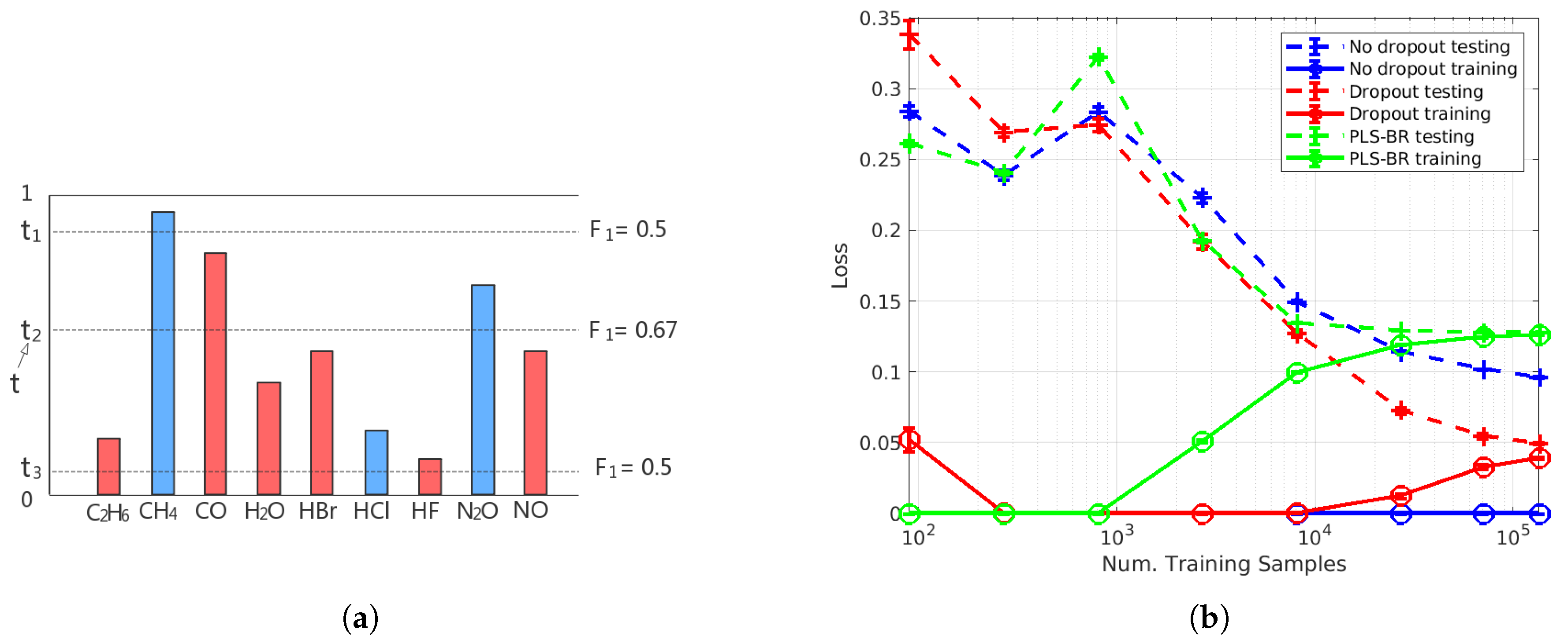
For binary classification problems in single-label learning, the sigmoid activation function of the output layer results in output scores that are between 0 and 1, and those output scores are often interpreted as the probabilities of the two possible classes. For each sample in the testing set, its predicted class will be the one with more than 0.5 probability (output score), so the classifier can be viewed as an FNN model with a threshold t = 0.5 . As shown in our Results Section, mislabelling of an extremely low concentration of a specific gas species as absent from the sample occurs more frequently than mislabelling a non-existing gas species as existing in the sample. This results in an imbalance between recall and precision. To re-balance recall and precision for higher F 1 , adopting an optimal threshold t for each label in each instance is desirable. For samples in the training set, the method of determining t is illustrated in Figure 4a. Suppose we have obtained output scores for all nine labels of a gas mixture. Three of them (blue ones) have the ground truth value of 1 (gas species exists in the sample), and the rest of the labels in red are 0 (gas species is absent in the sample). Then, we calculate the F 1 scores for the three candidates t 1 , t 2 and t 3 of t (dash lines), and the candidate with the highest F 1 score, which is t 2 in this example, is the t we need. In our model, we use output scores to calculate the candidates of t. For each sample, nine output scores will be formed into an increasing order: s 1 s 2 , , s 9 . Since the sigmoid function is used in the output layer, all output scores are between 0 and 1. Therefore, the ten threshold candidates will be:
0 , s 1 + s 2 2 , s 2 + s 3 2 , , s 8 + s 9 2 , 1
In order to get thresholds for all instances in the testing set systematically, we assume that threshold t is determined by the label scores s , and their relationship can be recognized by the following FNN model:
h t = f h ( W t ( 1 ) s + b t ( 1 ) ) t ^ = W t ( 2 ) h t + b t ( 2 )
where h t is a hidden layer with ReLU activation function f h and W t ( 1 ) , W t ( 2 ) , b t ( 1 ) and b t ( 2 ) are the parameters that need to be estimated. We will use instances in the training set to train the FNN model, and the loss function is the mean squared error between t and t ^ .

3.4. Evaluation Metrics

Hamming loss is a common evaluation metric for multi-label classification tasks. It is the fraction of the wrong predictions to the number of total gas labels of all testing samples. Mathematically, it is defined as:
H a m m i n g l o s s = 1 L · N i = 1 N j = 1 L F N i j + F P i j T N i j + T P i j + F N i j + F P i j
where T N i j , T P i j , F N i j and F P i j are true negatives, true positives, false negatives and false positives of the i th class of the j th label.
To evaluate our models, we also used micro-averaged recall, precision and F 1 as our figures of merit [10]. In our context, a true negative (TN) is the absence of a certain gas that has been correctly predicted in a sample. Similarly, a true positive (TP) is the case that an existing gas is marked as present in a sample. A false negative (FN) is the case that the classifier fails to identify an existing gas, and a false positive (FP) is a false alarm where the classifier identifies a non-existent gas.

4. Results and Discussions

4.1. Hyper-Parameter Tuning

In our research, we used TensorFlow to implement our FNN-OT and Adam as our optimizer. In the first step, we tuned hyper-parameters such as the dropout rate and training sample size of the FNN-OT model with the SNR = 30 dB dataset.

4.1.1. Dropout

In order to tune the hyper-parameters for dropout, a grid search was conducted on retention probabilities p = ( p 1 , p 2 ) of the input and hidden layers. A typical choice of retention rate is 0.8 for the input layer and 0.5 for the hidden layer [34], and a preliminary search on our datasets showed that the optimal choice of p was around (0.95, 0.2). More detailed tests on p 1 and p 2 were done around this point, and the results of all SNRs are shown in Figure 5. Combinations of p 1 and p 2 with the lowest Hamming loss will be applied to our model.

4.1.2. Training Sample Size

To determine the number of training samples that are sufficient for our models, we plotted the learning curve as shown in Figure 4b. Here, FNN-OT is compared with PLS-BR (Appendix B) and FNN with a 0.5 threshold.
As shown in the learning curves plot, we changed the number of samples in the training set while keeping the 20,000-sample testing set intact. Both training (solid lines) and testing (dashed lines) Hamming losses are plotted as a function of training samples. At an SNR of 30 dB , without dropout (blue markers), our FNN-OT model displayed large variance and low bias as the training loss was almost zero, while the testing loss was above 0.1 even when the training sample size was around 100,000. This is a clear indication of overfitting for training samples fewer than 100,000. In contrast, by adopting dropout (red markers), the overfitting issue was solved, and both training and testing loss converged to around 0.05 at around 100,000 training samples. In comparison, PLS-BR (green markers) did not display overfitting at the aforementioned sample size. However, the converged training and testing losses were higher (>0.1) than our FNN-OT model with dropout, indicating that our model outperformed this conventional technique. Nevertheless, the plot clearly showed that it was sufficient to use around 100,000 samples to train our FNN-OT with the dropout model.

4.2. Performance Comparison of Mutually Independent Gas Data

Parameters of PCA and FNN models will be trained in the 80,000-sample training sets and deployed in the 20,000-sample test sets.
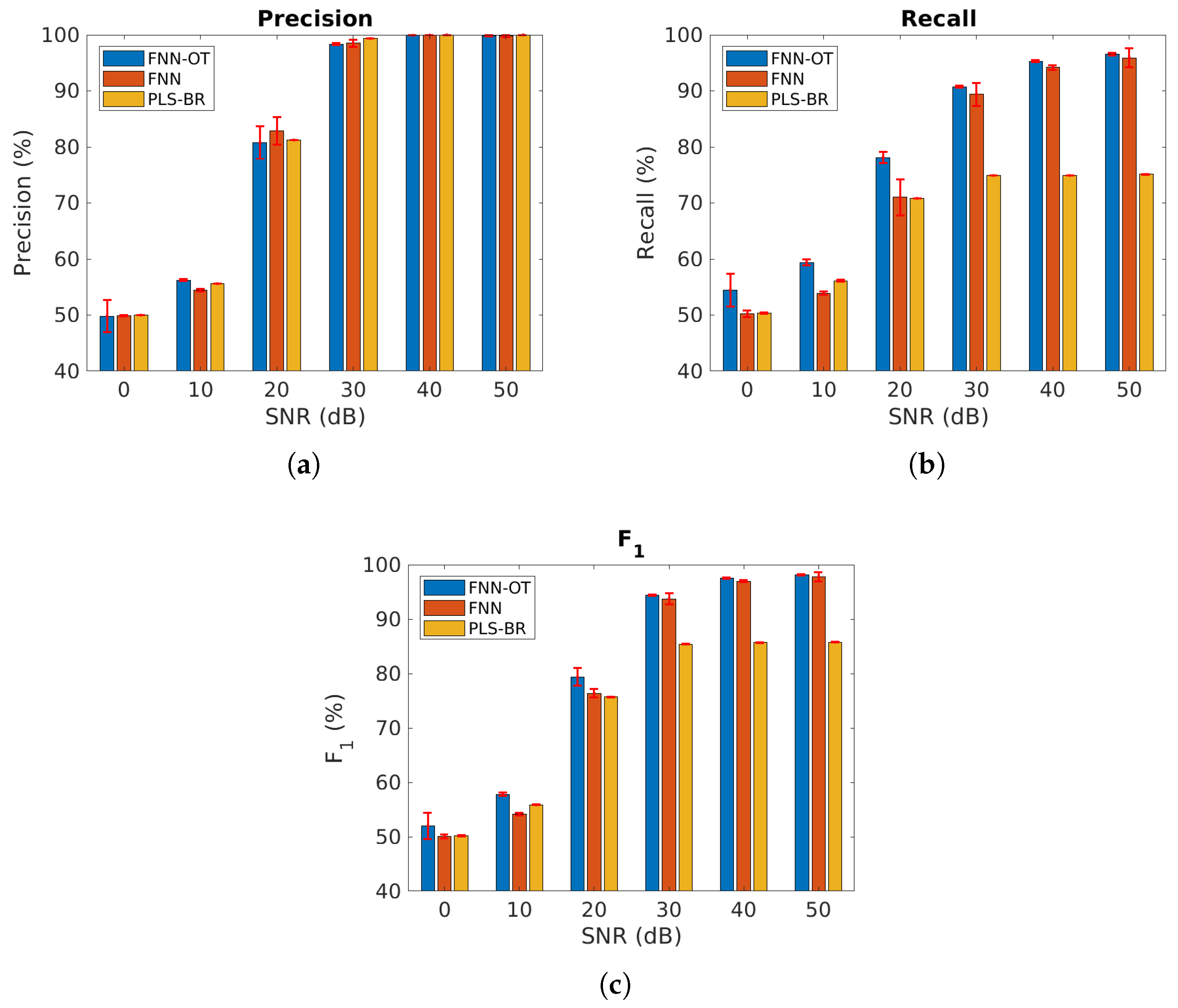
We first compared our model using the datasets where all gas components were mutually independent. Figure 6 and Table 1 present the micro-averaged precision, recall and F 1 score at six different SNRs. As expected, all models performed better at higher SNRs. When SNR was 0 dB , all three classifiers failed to identify gases because a 0.5 micro- F 1 score is as good as a random guess. Across all SNRs, FNN-OT yielded better precision, recall and F 1 than the conventional PLS-BR, clearly indicating it as a superior approach for gas identification.
FNN-OT also outperformed FNN in most cases at the cost of slightly longer computing time. It took FNN-OT around 640 s to complete one of the 10 folds, and for FNN, the computing time was about 430 s. In some cases, when the SNR was 0 dB , FNN-OT had slightly lower precision compared to FNN. This resulted from the optimal thresholding system where thresholds were the ones that could maximize the F 1 scores. FNN-OT scarified precision to reach a higher overall F 1 score. Figure 6 also illustrates that all three models displayed higher values of precision than recall. This was due to the fact that most mislabelling occurred when a gas species’ concentration was too low to produce a detectable signal above the noise background, and all model would mistakenly predict the absence of that gas and produce an FN. However, as is evident from Figure 6b, selecting the optimal threshold would significantly reduce the occurrence of FN and increase recall without significantly reducing the precision, resulting in a better F 1 score. This clearly justified the necessity of adopting FNN-OT.
The advantages of FNN-OT were further confirmed by comparing the minimum detectable concentrations of nine gases as in Figure 7. As shown, both FNN-OT and FNN consistently showed lower minimum detectable concentration at all SNRs, while in general, FNN-OT outperformed FNN.

4.3. Performance Comparison for Highly Correlated Gas Data

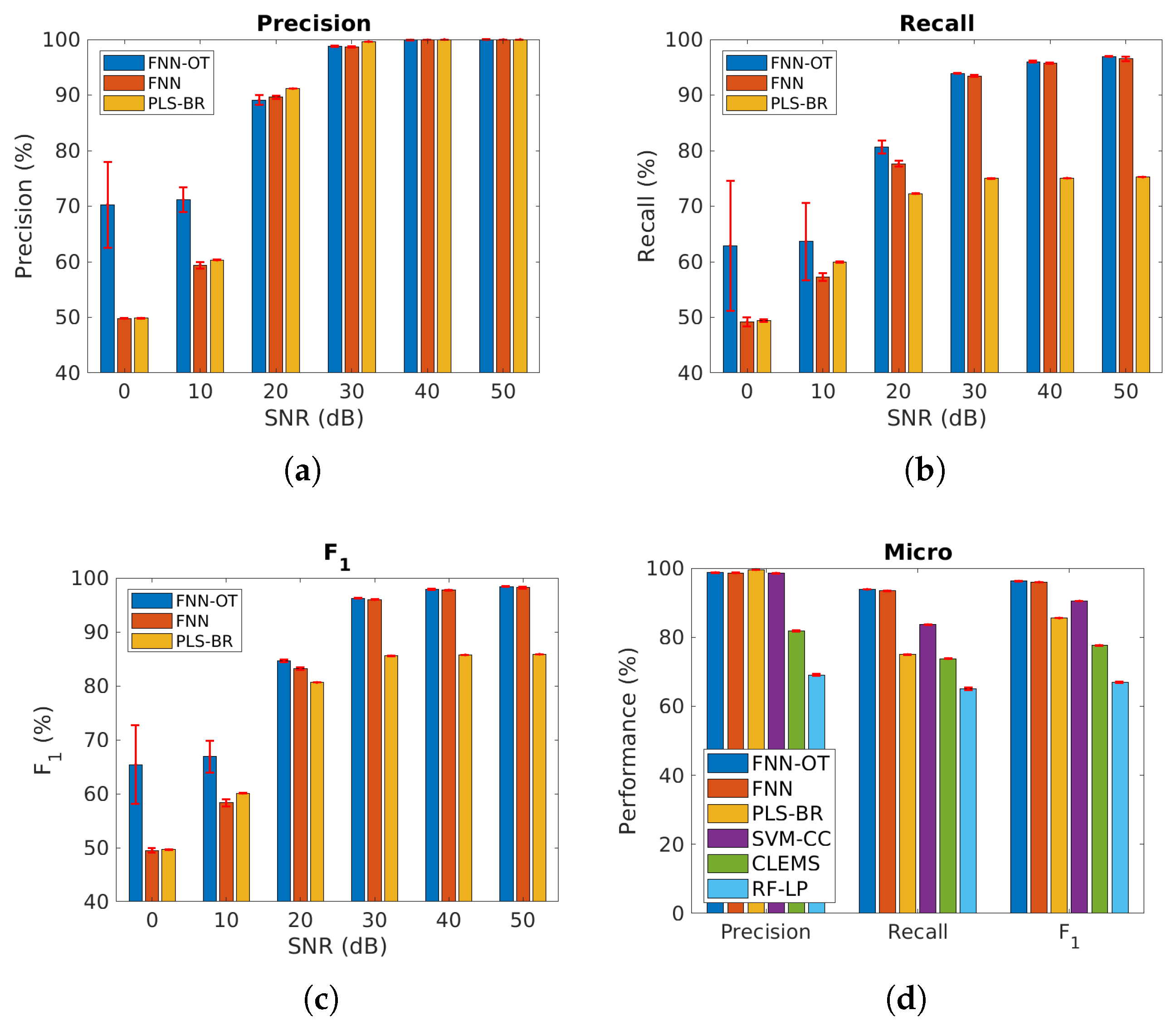
We further applied our models to the cases when the gases were correlated. As shown in Figure 8a–c and Table 2, when SNR was above 20 dB , the performance of the three models was similar to the uncorrelated case, and FNN-OT outperformed. Further, at SNR = 0 dB or 10 dB , FNN-OT significantly outperformed the other two models and its own results of the uncorrelated case due to the fact that FNN-OT could collaboratively identify gas species by organizing their correlation, while FNN and PLS-BR were not capable of this. Since PLS-BR ignored label correlations completely, in Figure 8d and Table 3, three models, support vector machine-classifier chains (SVM-CC), cost-sensitive label embedding with multidimensional scaling (CLEMS) and random forest-label powerset (RF-LP), were added as additional base models for comparison. SVM-CC is the combination of a common classifier support vector machine (SVM) and a problem transformation method classifier chains (CC), where CC exploits label correlation information with a chain of classifiers. CLEMS is a well performing label embedding method that transforms original labels into new embedded space. Along with CLEMS, we applied the random forest regressor and the multi-label k-nearest neighbor (MLKNN) classifier, which is a common combination used for label embedding. RF-LP uses the label powerset to map the combinations of original labels into new single labels for random forest to classify. The results in Figure 8d show that SVM-CC, CLEMS and RF-LP had lower micro-averaged precision, recall and F 1 score compared to FNN-OT.
All models were trained and tested on a home assembled desktop computer that had 64 GB DDR4 memory, a Micro-Star Z370 Gaming Plus motherboard and a 3.20 GHz Intel i7-8700 CPU with 12 units of processors. It had two graphics processing units (GPUs) installed: one was an NVidia GeForce GTX 1070 with 1920 CUDA cores and 8 GB GDDR5 memory, and the other was an NVidia GeForce GTX 1050 with 768 CUDA cores and 4 GB GDDR5 memory. Here, both FNN and FNN-OT were implemented using Google’s TensorFlow and trained on the GTX 1070 GPU. Other models were implemented using skicit-learn and skicit-multilearn packages and trained on a CPU. During training of FNN and FNN-OT, the typical volatile GPU utilization was around 64%, and the typical CPU load was around 5.0 when training other models. The computing time of one of the 10-fold cross-validations for all six models is compared in the last column of Table 3. With the assistance of the GPU, FNN-OT outperformed SVM-CC, CLEMS and RF-LP in computing time. On the other hand, PLS-BR had the shortest computing time of 100 s. The computing time of CLEMS was the longest (about 3.5 h) among all models.

5. Conclusions

In conclusion, by selecting optimal thresholds, FNN-OT outperformed conventional PLS-BR, SVM-CC, CLEMS and FNN in two aspects. FNN-OT could dynamically select a threshold to reduce FN events. In addition, FNN-OT was capable of utilizing the correlation among the components to enhance its classification capability. Both of these unique features make FNN-OT a favourable choice for spectroscopic analysis in cluttered environments.

Author Contributions

Conceptualization, T.L.; methodology, T.L. and L.G.; software, L.G., B.Y. and T.L.; validation, L.G., B.Y. and T.L.; formal analysis, L.G., B.Y. and T.L.; investigation, L.G., B.Y. and T.L.; resources, T.L.; data curation, T.L.; writing, original draft preparation, L.G.; writing, review and editing, L.G., B.Y. and T.L.; visualization, L.G. and B.Y.; supervision, T.L.; project administration, T.L.; funding acquisition, T.L.

Funding

This research was funded by the Nature Science and Engineering Research Council of Canada (NSERC) Discovery (Grant No. RGPIN-2015-06515), Defense Threat Reduction Agency (DTRA) Thrust Area 7, Topic G18 (Grant No. GRANT12500317), and the Nvidia Corporation TITAN-X GPU grant.

Acknowledgments

The authors would like to thank Kerry Vahala and Qiang Lin for their helpful discussions.

Conflicts of Interest

The authors declare no conflict of interest.

Appendix A. Generation of Correlated Uniformly Distributed Random Variables
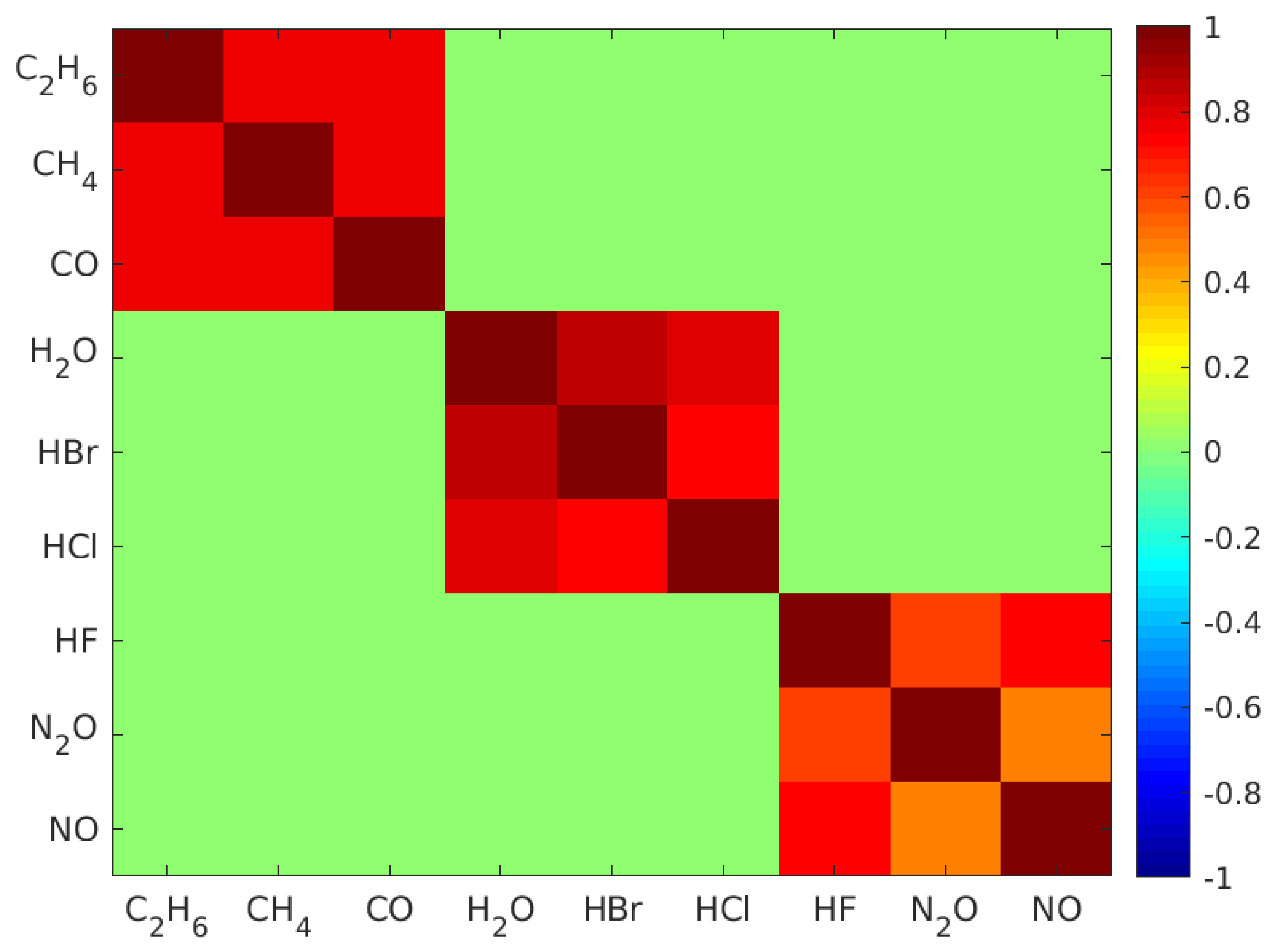
To test our models with highly correlated gas labels, we constructed a correlation matrix of all nine gases. To simplify our model, we evenly divided nine gases into three subsets and generated highly correlated uniformly distributed random concentrations of the three gases in each subset. The correlation matrix at SNR = 30 dB is illustrated in Figure A1.
Figure A1. Correlation matrix of nine gases at SNR = 30 dB .
Make 01 00061 g0a1
Firstly, we generated covariance matrix Σ of the nine variables, which had to be symmetric positive semi-definite. Let:
L = 100 L ˜ 11 L 12 L 13 L 21 100 L 22 L 23 L 31 L 32 100 L 33
where L ij are 3 × 3 random matrices with element values uniformly distributed between ( 0 , 1 ) . Then, Σ = LL T will be symmetric positive semi-definite. With the covariance matrix, one may easily obtain the corresponding multivariate normal random numbers X i through, e.g., MATLAB’s mvnrnd command. To generate uniformly distributed random numbers Y i from the above multivariate normal random numbers X i , we used the approach in [36]. The procedure is as follows: define x i j , ( j = 1 , , N i ) as the j th random number of X i , ( i = 1 , 2 ) . N i is the total number of samples in random variable X i . First, compute the cumulative distributed function P c d f i of X i according to:
P c d f i ( x ) = 1 N i Σ 1 N i 1 ( x i j < x )
Here, 1 ( x i j < x ) is an indicator function that returns one if the condition in the bracket holds and zero otherwise. Consequently, the uniformly distributed random variable Y i , ( i = 1 , 2 ) can be easily constructed according to:
Y i = P c d f i ( X i )
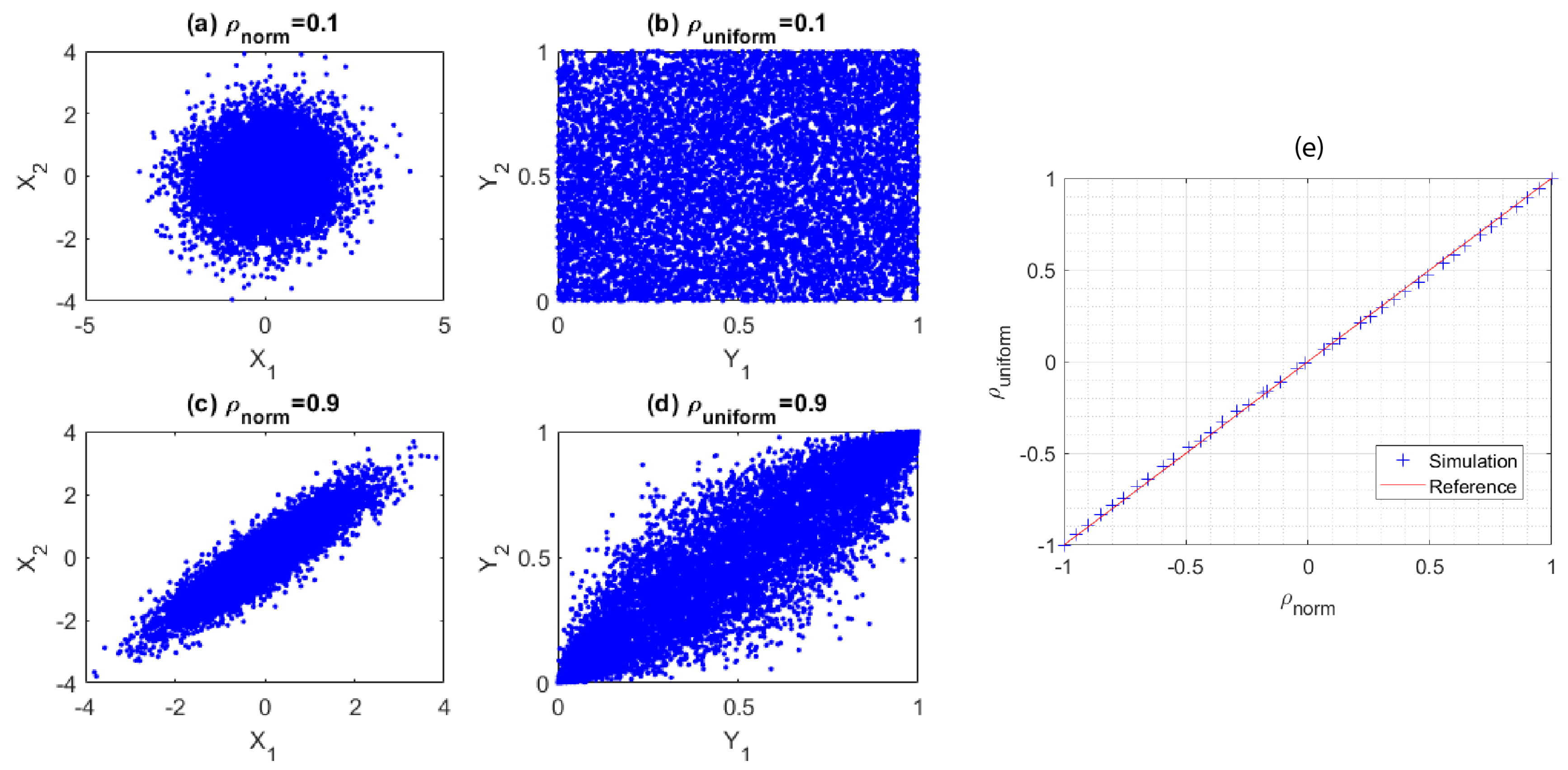
Figure A2 clearly shows the validity of the procedure. Here, the joint distribution of two partially correlated normal distributed random variables X 1 and X 2 with correlation coefficients 0.1 and 0.9 are plotted in Subplots (a) and (c), respectively. The distribution of the corresponding transformed uniformly distributed random variables Y 1 and Y 2 are shown in Subplots (b) and (d), with correlation coefficient values retained after transformation. Figure A2e further plots the correlation coefficients of Y vs. the coefficients of X. As shown, the transformed correlation coefficients are almost identical to the coefficients of their original pair.
Figure A2. Joint distribution of two normal distributed random variables X 1 and X 2 with correlation coefficient (a) ρ n o r m = 0.1 and (b) ρ n o r m = 0.9 . The joint distribution of transformed uniform distributed random variables Y 1 and Y 2 is plotted in (c) and (d), respectively, with correlation retained. (e) The correlation coefficients of transformed random variables vs. the coefficients of the original normal distributed random variables.
Make 01 00061 g0a2

Appendix B. Partial Least Squares Method

Our model was compared with conventional PLS-BR. PLS-BR is a multi-label classifier adapted from PLS. It utilizes BR to split the multi-label task into several single-label classification problems. BR decomposes the learning of output labels into a set of binary classification tasks, one per label, where each single model is learned independently, using only the information of that particular label and ignoring the information of all other labels [37]. It has various advantages such as the base learner can be selected from any of the binary learning methods, and also, the complexity is linear with the number of labels. Apart from this, it can also optimize several loss functions. The main disadvantage of BR is that it assumes that all labels are independent and ignores the correlations between them.
PLS is a widely used quantitative technique in advanced spectral analysis [38]. In order to predict output Y from feature X, PLS describes the common structure of X and Y by combining PCA and multivariate regression [39]. Similar to PCA, PLS decomposes X and Y as follows:
X = T P T Y = U Q T
where T and U are projections of X and Y and P T and Q T are the transpose of orthogonal loading matrices. Then, regression of T and U will be performed following the standard multivariate regression procedure.
PLS itself is not designed for classification, so an extension of PLS called PLS-DA (partial least squares-discriminant analysis) was adopted to classify categorical outputs. PLS-DA was successfully used to classify milk and lubricant based on spectroscopic datasets in [40,41,42]. In binary classification ( y = 0 or 1) cases, PLS-DA creates two dummy variables y 1 ( y = 0 ) and y 2 ( y = 1 ) for the y label and then calculates the PLS regression scores for y 1 and y 2 . If y 1 has a higher score, y is classified as zero. Otherwise, the prediction class of y is one.

References

  1. Gallagher, M.; Deacon, P. Neural networks and the classification of mineralogical samples using X-ray spectra. In Proceedings of the 2002 9th International Conference on Neural Information Processing (ICONIP’02), Singapore, 18–22 November 2002; IEEE: Piscataway, NJ, USA, 2002; Volume 5, pp. 2683–2687. [Google Scholar]
  2. Jiang, J.; Zhao, M.; Ma, G.-M.; Song, H.-T.; Li, C.-R.; Han, X.; Zhang, C. Tdlas-based detection of dissolved methane in power transformer oil and field application. IEEE Sens. J. 2018, 18, 2318–2325. [Google Scholar] [CrossRef]
  3. Dong, D.; Jiao, L.; Li, C.; Zhao, C. Rapid and real-time analysis of volatile compounds released from food using infrared and laser spectroscopy. TrAC Trends Anal. Chem. 2019, 110, 410–416. [Google Scholar] [CrossRef]
  4. Christy, C.D. Real-time measurement of soil attributes using on-the-go near infrared reflectance spectroscopy. Comput. Electron. Agric. 2008, 61, 10–19. [Google Scholar] [CrossRef]
  5. Wang, Y.; Wei, Y.; Liu, T.; Sun, T.; Grattan, K.T. Tdlas detection of propane/butane gas mixture by using reference gas absorption cells and partial least square approach. IEEE Sens. J. 2018, 18, 8587–8596. [Google Scholar] [CrossRef]
  6. Schumacher, W.; Kühnert, M.; Rösch, P.; Popp, J. Identification and classification of organic and inorganic components of particulate matter via raman spectroscopy and chemometric approaches. J. Raman Spectrosc. 2011, 42, 383–392. [Google Scholar] [CrossRef]
  7. Goodacre, R. Explanatory analysis of spectroscopic data using machine learning of simple, interpretable rules. Vib. Spectrosc. 2003, 32, 33–45. [Google Scholar] [CrossRef]
  8. Yang, Y. An evaluation of statistical approaches to text categorization. Inf. Retr. 1999, 1, 69–90. [Google Scholar] [CrossRef]
  9. Schapire, R.E.; Singer, Y. Boostexter: A boosting-based system for text categorization. Mach. Learn. 2000, 39, 135–168. [Google Scholar] [CrossRef]
  10. Tsoumakas, G.; Katakis, I. Multi-label classification: An overview. Int. J. Data Warehous. Min. 2006, 3, 1–13. [Google Scholar] [CrossRef]
  11. Gibaja, E.; Ventura, S. Multi-label learning: A review of the state of the art and ongoing research. Wiley Interdiscip. Rev. Data Min. Knowl. Discov. 2014, 4, 411–444. [Google Scholar] [CrossRef]
  12. Zhang, Y.; Schneider, J. Maximum margin output coding. In Proceedings of the 29th International Coference on International Conference on Machine Learning (ICML’12), Edinburgh, UK, 26 June–1 July 2012; Omnipress: Madison, WI, USA, 2012; pp. 379–386. [Google Scholar]
  13. Zhang, M.; Wu, L. Lift: Multi-label learning with label-specific features. IEEE Trans. Pattern Anal. Mach. Intell. 2015, 37, 107–120. [Google Scholar] [CrossRef] [PubMed]
  14. Zhang, M.-L.; Zhang, K. Multi-label learning by exploiting label dependency. In Proceedings of the 16th ACM SIGKDD International Conference on Knowledge Discovery and Data Mining (KDD ’10), Washington, DC, USA, 25–28 July 2010; ACM: New York, NY, USA, 2010; pp. 999–1008. [Google Scholar] [CrossRef]
  15. Li, Q.; Xie, B.; You, J.; Bian, W.; Tao, D. Correlated logistic model with elastic net regularization for multilabel image classification. IEEE Trans. Image Process. 2016, 25, 3801–3813. [Google Scholar] [CrossRef] [PubMed]
  16. Li, Q.; Qiao, M.; Bian, W.; Tao, D. Conditional graphical lasso for multi-label image classification. In Proceedings of the 2016 IEEE Conference on Computer Vision and Pattern Recognition (CVPR), Las Vegas, NV, USA, 27–30 June 2016; pp. 2977–2986. [Google Scholar]
  17. Godbole, S.; Sarawagi, S. Discriminative Methods for Multi-Labeled Classification. In Advances in Knowledge Discovery and Data Mining; Springer: Berlin/Heidelberg, Germany, 2004; pp. 22–30. [Google Scholar]
  18. Katakis, I.; Tsoumakas, G.; Vlahavas, I. Multilabel text classification for automated tag suggestion. In Proceedings of the ECML PKDD Discovery Challenge, Antwerp, Belgium, 15–19 September 2008; Volume 75. [Google Scholar]
  19. Tsoumakas, G.; Vlahavas, I. Random k-Labelsets: An Ensemble Method for Multilabel Classification. In European Conference on Machine Learning; Springer: Berlin/Heidelberg, Germany, 2007; pp. 406–417. [Google Scholar]
  20. Read, J.; Pfahringer, B.; Holmes, G.; Frank, E. Classifier Chains for Multi-Label Classification. In Machine Learning and Knowledge Discovery in Databases; Springer: Berlin/Heidelberg, Gemany, 2009; pp. 254–269. [Google Scholar]
  21. Huang, K.H.; Lin, H.T. Cost-sensitive label embedding for multi-label classification. Mach. Learn. 2017, 106, 1725–1746. [Google Scholar] [CrossRef] [Green Version]
  22. Szymański, P.; Kajdanowicz, T.; Chawla, N. LNEMLC: Label Network Embeddings for Multi-Label Classifiation. arXiv 2018, arXiv:1812.02956. [Google Scholar]
  23. Szymański, P.; Kajdanowicz, T.; Kersting, K. How is a data-driven approach better than random choice in label space division for multi-label classification? Entropy 2016, 18, 282. [Google Scholar] [CrossRef]
  24. Clare, A.; King, R.D. Knowledge Discovery in Multi-Label Phenotype Data. In European Conference on Principles of Data Mining and Knowledge Discovery; Springer: Berlin/Heidelberg, Germany, 2001; pp. 42–53. [Google Scholar]
  25. Zhang, M.-L.; Zhou, Z.-H. A k-nearest neighbor based algorithm for multi-label classification. In Proceedings of the 2005 IEEE International Conference on Granular Computing, Beijing, China, 25–27 July 2005; IEEE: Piscataway, NJ, USA, 2005; Volume 2, pp. 718–721. [Google Scholar]
  26. Younes, Z.; Abdallah, F.; Denœux, T. Multi-label classification algorithm derived from k-nearest neighbor rule with label dependencies. In Proceedings of the 2008 16th European Signal Processing Conference, Lausanne, Switzerland, 25–29 August 2008; IEEE: Piscataway, NJ, USA, 2008; pp. 1–5. [Google Scholar]
  27. Read, J.; Hollmén, J. Multi-label classification using labels as hidden nodes. arXiv 2015, arXiv:1503.09022. [Google Scholar]
  28. Zhang, M.-L.; Zhou, Z.-H. Multilabel neural networks with applications to functional genomics and text categorization. IEEE Trans. Knowl. Data Eng. 2006, 18, 1338–1351. [Google Scholar] [CrossRef]
  29. Nam, J.; Kim, J.; Mencía, E.L.; Gurevych, I.; Fürnkranz, J. Large-Scale Multi-Label Text Classification- Revisiting Neural Networks. In Joint European Conference on Machine Learning and Knowledge Discovery in Databases; Springer: Berlin/Heidelberg, Germany, 2014; pp. 437–452. [Google Scholar]
  30. Collobert, R.; Weston, J. A unified architecture for natural language processing: Deep neural networks with multitask learning. In Proceedings of the 25th International Conference on Machine Learning, Helsinki, Finland, 5–9 July 2008; ACM: New York, NY, USA, 2008; pp. 160–167. [Google Scholar]
  31. Gong, Y.; Jia, Y.; Leung, T.; Toshev, A.; Ioffe, S. Deep convolutional ranking for multilabel image annotation. arXiv 2013, arXiv:1312.4894. [Google Scholar]
  32. Wang, J.; Yang, Y.; Mao, J.; Huang, Z.; Huang, C.; Xu, W. Cnn-rnn: A unified framework for multi-label image classification. In Proceedings of the IEEE Conference on Computer Vision and Pattern Recognition, Las Vegas, NV, USA, 27–30 June 2016; pp. 2285–2294. [Google Scholar]
  33. Rothman, L.S.; Gordon, I.E.; Babikov, Y.; Barbe, A.; Benner, D.C.; Bernath, P.F.; Birk, M.; Bizzocchi, L.; Boudon, V.; Brown, L.R.; et al. The HITRAN 2012 Molecular Spectroscopic Database. J. Quant. Spectrosc. Radiat. Transf. 2013, 130, 4–50. [Google Scholar] [CrossRef]
  34. Srivastava, N.; Hinton, G.; Krizhevsky, A.; Sutskever, I.; Salakhutdinov, R. Dropout: A simple way to prevent neural networks from overfitting. J. Mach. Learn. Res. 2014, 15, 1929–1958. [Google Scholar]
  35. Holland, S.M. Principal Components Analysis (PCA); Department of Geology, University of Georgia: Athens, GA, USA, 2008. [Google Scholar]
  36. Allred, C.S. Partially Correlated Uniformly Distributed Random Numbers. Available online: https://medium.com/capital-one-tech/partially-correlated-uniformly-distributed-random-numbers-5ce82486b68a (accessed on 1 November 2019).
  37. Luaces, O.; Díez, J.; Barranquero, J.; del Coz, J.J.; Bahamonde, A. Binary relevance efficacy for multilabel classification. Prog. Artif. Intell. 2012, 1, 303–313. [Google Scholar] [CrossRef] [Green Version]
  38. Madden, M.G.; Howley, T. A Machine Learning Application for Classification of Chemical Spectra. In Applications and Innovations in Intelligent Systems XVI; Springer: London, UK, 2009; pp. 77–90. [Google Scholar] [Green Version]
  39. Geladi, P.; Kowalski, B.R. Partial least-squares regression: A tutorial. Anal. Chim. Acta 1986, 185, 1–17. [Google Scholar] [CrossRef]
  40. Elbassbasi, M.; Kzaiber, F.; Ragno, G.; Oussama, A. Classification of raw milk by infrared spectroscopy (ftir) and chemometric. J. Sci. Specul. Res. 2010, 1, 28–33. [Google Scholar]
  41. Hirri, A.; Bassbasi, M.; Oussama, A. Classification and quality control of lubricating oils by infrared spectroscopy and chemometric. Int. J. Adv. Technol. Eng. Res. 2013, 3, 59–62. [Google Scholar]
  42. Hirri, A.; Bassbasi, M.; Platikanov, S.; Tauler, R.; Oussama, A. Ftir spectroscopy and pls-da classification and prediction of four commercial grade virgin olive oils from morocco. Food Anal. Methods 2016, 9, 974–981. [Google Scholar] [CrossRef]
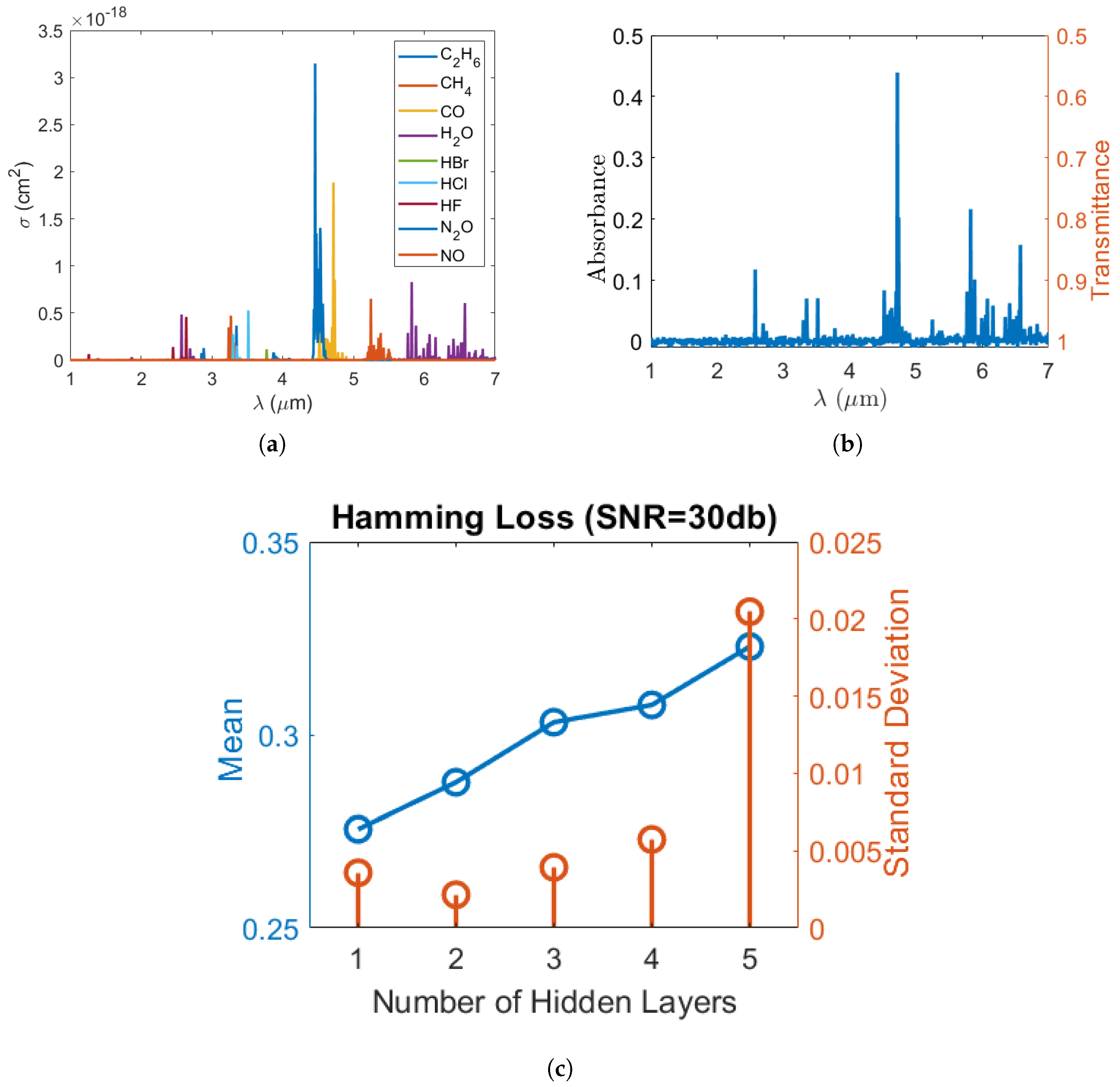
Figure 1. (a) Absorption cross-section of each gas molecule as a function of wavelength ( λ ); (b) the absorption/transmission spectrum of a sample gas mixture at SNR = 30 dB and (c) Hamming loss vs. the number of hidden layers when the SNR is 30 dB and gas labels are independent.
Make 01 00061 g001
Figure 2. (a) FNN-optimal thresholding (OT) training and testing procedure. (b) A typical FNN model with dropout.
Make 01 00061 g002
Figure 3. (a) Percentage of cumulative explained variance vs. number of principal components adopted at SNR = 40 dB . (b) Comparison of Hamming loss with and without PCA and dropout at SNR = 40 dB .
Make 01 00061 g003
Figure 4. (a) Illustration of optimal thresholding. (b) Learning curves of FNN-OT without dropout (blue), with dropout (red) and PLS-binary relevance (BR) (green).
Make 01 00061 g004
Figure 5. Hamming loss vs. retention probability, assuming all gases are independent.
Make 01 00061 g005
Figure 6. Micro-averaged (a) precision, (b) recall and (c) F 1 score at different SNRs, assuming all gases are independent. Red error bars represent standard deviations of the 10-fold cross-validation tests. Numerical results are presented in Table 1.
Make 01 00061 g006
Figure 7. Minimum detectable concentration ( C m i n ) of nine gases at (a) SNR = 0 dB, (b) SNR = 10 dB, (c) SNR = 20 dB, (d) SNR = 30 dB, (e) SNR = 40 dB and (f) SNR = 50 dB.
Make 01 00061 g007
Figure 8. Micro-averaged (a) precision, (b) recall and (c) F 1 score of the same three models as in Figure 6 at different SNRs, assuming some of the gases are highly correlated. (d) Micro-averaged metrics for six models at SNR = 30 dB . Red error bars represent standard deviations of the 10-fold cross-validation tests. Numerical results are presented in Table 2 and Table 3. CC, classifier chains; CLEMS, cost-sensitive label embedding with multidimensional scaling; LP, label powerset.
Make 01 00061 g008
Table 1. Numerical results of Figure 6a–c.
Micro-Averaged Precision
FNN-OTFNNPLS-BR
0 dB 0.50 ± 0.030.499 ± 0.0010.4998 ± 0.0004
10 dB 0.562 ± 0.0020.545 ± 0.0030.5561 ± 0.0004
20 dB 0.81 ± 0.030.83 ± 0.020.8124 ± 0.0003
30 dB 0.983 ± 0.0020.985 ± 0.0060.9935 ± 0.0001
40 dB 0.9992 ± 0.00020.9996 ± 0.00011 ± 0
50 dB 0.998 ± 0.0010.998 ± 0.0021 ± 0
Micro-Averaged Recall
FNN-OTFNNPLS-BR
0 dB 0.54 ± 0.030.502 ± 0.0060.504 ± 0.001
10 dB 0.594 ± 0.0050.539 ± 0.0030.561 ± 0.001
20 dB 0.78 ± 0.010.71 ± 0.030.7083 ± 0.0003
30 dB 0.908 ± 0.0020.89 ± 0.020.7488 ± 0.0002
40 dB 0.953 ± 0.0020.942 ± 0.0040.7492 ± 0.0003
50 dB 0.965 ± 0.0030.96 ± 0.020.7507 ± 0.0002
Micro-Averaged F 1 Score
FNN-OTFNNPLS-BR
0 dB 0.52 ± 0.020.501 ± 0.0030.5017 ± 0.0007
10 dB 0.578 ± 0.0030.542 ± 0.0030.5587 ± 0.0008
20 dB 0.79 ± 0.020.764 ± 0.0080.7568 ± 0.0003
30 dB 0.9439 ± 0.00070.94 ± 0.010.8539 ± 0.0002
40 dB 0.9755 ± 0.00090.970 ± 0.0020.8566 ± 0.0002
50 dB 0.981 ± 0.0020.978 ± 0.0090.8576 ± 0.0001
Table 2. Micro-averaged metrics of highly correlated gas data at different SNRs.
Micro-Averaged Precision
FNN-OTFNNPLS-BR
0 dB 0.70 ± 0.080.4979 ± 0.00080.498 ± 0.001
10 dB 0.71 ± 0.020.594 ± 0.0060.6030 ± 0.0005
20 dB 0.89 ± 0.010.896 ± 0.0030.9114 ± 0.0003
30 dB 0.987 ± 0.0010.987 ± 0.0010.9961 ± 0.0001
40 dB 0.9989 ± 0.00030.9991 ± 0.00021 ± 0
50 dB 0.9996 ± 0.00050.9998 ± 0.00010.9926 ± 0.0007
Micro-Averaged Recall
FNN-OTFNNPLS-BR
0 dB 0.6 ± 0.10.492 ± 0.0080.495 ± 0.002
10 dB 0.64 ± 0.070.573 ± 0.0070.599 ± 0.001
20 dB 0.81 ± 0.010.777 ± 0.0050.7232 ± 0.0004
30 dB 0.9388 ± 0.00070.934 ± 0.0020.7497 ± 0.0003
40 dB 0.960 ± 0.0020.957 ± 0.0010.7505 ± 0.0002
50 dB 0.9692 ± 0.00070.965 ± 0.0040.7497 ± 0.0002
Micro-Averaged F 1 Score
FNN-OTFNNPLS-BR
0 dB 0.65 ± 0.070.495 ± 0.0040.496 ± 0.001
10 dB 0.67 ± 0.030.583 ± 0.0070.6011 ± 0.0007
20 dB 0.846 ± 0.0030.832 ± 0.0020.8064 ± 0.0002
30 dB 0.9625 ± 0.00040.9597 ± 0.00060.8555 ± 0.0002
40 dB 0.9791 ± 0.00090.9776 ± 0.00060.8575 ± 0.0002
50 dB 0.9841 ± 0.00040.9821 ± 0.00200.8542 ± 0.0004
Table 3. Micro-averaged metrics and computing time of highly correlated gas data at SNR =  30 dB . FNN-OT and FNN were trained on a GPU. Other models were trained on a CPU.
PrecisionRecall F 1 ScoreComputing Time
FNN-OT0.987 ± 0.0010.9388 ± 0.00070.9625 ± 0.0004640 s
FNN0.987 ± 0.0010.934 ± 0.0020.9597 ± 0.0006440 s
PLS-BR0.9961 ± 0.00010.7497 ± 0.00030.8555 ± 0.0002100 s
SVM-CC0.9855 ± 0.00070.8365 ± 0.00090.9049 ± 0.00041440 s
CLEMS0.819 ± 0.0020.738 ± 0.0020.7765 ± 0.000812,000 s
RF-LP0.691 ± 0.0020.650 ± 0.0040.670 ± 0.002720 s