A Radiative Transfer Model-Based Multi-Layered Regression Learning to Estimate Shadow Map in Hyperspectral Images

Abstract

The application of Empirical Line Method (ELM) for hyperspectral Atmospheric Compensation (AC) premises the underlying linear relationship between a material’s reflectance and appearance. ELM solves the Radiative Transfer (RT) equation under specialized constraint by means of in-scene white and black calibration panels. The reflectance of material is invariant to illumination. Exploiting this property, we articulated a mathematical formulation based on the RT model to create cost functions relating variably illuminated regions within a scene. In this paper, we propose multi-layered regression learning-based recovery of radiance components, i.e., total ground-reflected radiance and path radiance from reflectance and radiance images of the scene. These decomposed components represent terms in the RT equation and enable us to relate variable illumination. Therefore, we assume that Hyperspectral Image (HSI) radiance of the scene is provided and AC can be processed on it, preferably with QUick Atmospheric Correction (QUAC) algorithm. QUAC is preferred because it does not account for surface models. The output from the proposed algorithm is an intermediate map of the scene on which our mathematically derived binary and multi-label threshold is applied to classify shadowed and non-shadowed regions. Results from a satellite and airborne NADIR imagery are shown in this paper. Ground truth (GT) is generated by ray-tracing on a LIDAR-based surface model in the form of contour data, of the scene. Comparison of our results with GT implies that our algorithm’s binary classification shadow maps outperform other existing shadow detection algorithms in true positive, which is the detection of shadows when it is in ground truth. It also has the lowest false negative i.e., detecting non-shadowed region as shadowed, compared to existing algorithms.

1. Introduction

A high-fidelity hyperspectral imagery contains crucial spatial and spectral information of a given scene. Presence of shadows causes significant challenges for both satellite and airborne data analyses. Shadows cast by scene geometry or clouds cause hurdles in remote-sensing data analyses, including inaccurate atmospheric compensation, biased estimation of Normalized Difference Vegetation Index (NDVI), confusion in land cover classification, and anomalous detection of landcover variation. Therefore, shadows are a significant source of noise in Hyperspectral Image (HSI) data, and their detection is a vital pre-processing step in most analyses [1,2].

Over the years, various methods of shadow detection proposed are object-based shadow detection methods which classify clouds, their shadows, and non-shadowed regions by applying image segmentation at different bandwidth images of HSI imagery, e.g., [3,4], and color invariance-based shadow detection methods create RGB in invariant color space and exploit it for classification as in [5]. Some algorithms use band indices to detect shadows in an HSI image [6,7]. Another class of algorithms require an a priori Digital Surface Model (DSM) [8] or Terrestrial Laser Scanning data together with the HSI image to find shadows cast from scene geometry [9].

Beril et al. [10] proposed a color-invariant function for detecting buildings. Once buildings are detected, then they used the grayscale histogram of the image to detect shadows around the building using the Otsu algorithm [11], their algorithm is referred to as Beril’s algorithm in the results. In another contribution, Teke et al. [12] proposed a false color space consisting of red, green and near infrared (NIR) bands. They dropped the blue color because it contains scattered light and removing it will increase the contrast between shadow and non-shadow regions, and will facilitate detection. They have named their algorithm the Land Use Land Cover classification method, or LULC in their code. Therefore, we will refer to their work as LULC algorithm in our analysis. Sevim et al. [13] modified the $C_1$,$C_2$,$C_3$ color space [14] to accommodate the NIR band, and supplemented it to become the $C_1^{\prime }$,$C_2^{\prime }$,$C_3^{\prime }$,$C_4^{\prime }$ color space. We refer to their work as RGBN algorithm. Gevers et al. [15] proposed color-invariance functions to separate shadow and non-shadow regions; their algorithm is referred to as Gevers’ algorithm.

The approaches mentioned above are limited to use in particular bands, and may not use the complete hyperspectral data. Our algorithm may ideally use HSI data and can be down-scaled to multispectral imagery only in cases where data-acquisition sensor response is known. Spectral response is typically available for most Earth-observation satellites. Our algorithm does not address RGB images because QUAC [16] may not be applied to retrieve reflectance from RGB images. More importantly, our algorithm provides a mathematical foundation for shadow detection based on the RT model and highlights the sources of errors. Retrieval of radiance components by machine learning enables it to be extended for shadow compensation.

2. Radiative Transfer Model-Based Relationship between Shadowed and Non-Shadowed Regions

The scope of this research is within optical shadowing, and therefore, the subsequent discussion does not consider thermal radiance and shadowing and their relative terms in Radiative Transfer (RT) equations. This section is divided into two parts—the first presents a general description of the RT equation highlighting relevant parameters and elaborating the sources of errors and their impact on this work, and the second establishes the proposed general relationship between variably illuminated regions based on the RT equation.

2.1. Radiative Transfer Equation

The RT equation for at-sensor radiance within an optical spectrum is given as Equation (1), [17].

$$\begin{array}{c}Ls({\theta }_i,{\theta }_r,\varphi ,\rho ,{\mathsf{\Omega }}_i)=\hfill \\ \hfill f_r({\theta }_i,{\theta }_r,\varphi )E_s\left({\theta }_i\right)cos\left({\theta }_i\right){\tau }_i\left({\theta }_i\right){\tau }_r\left({\theta }_r\right)\rho +{\tau }_r\left({\theta }_r\right)\rho {\int }_F\int {\int }_{{\mathsf{\Omega }}_i}{f}_r({\theta }_i,{\theta }_r,\varphi )cos\left({\theta }_i\right)L_d^{{\mathsf{\Omega }}_i}({\theta }_i,\varphi )d{\mathsf{\Omega }}_i+L_p({\theta }_i,\varphi )\end{array}$$

(1)

where $Ls$ is total at-sensor radiance, $f_r$ is the Bidirectional Reflection Distribution Function (BRDF) [18], $E_s$ is exoatmospheric solar spectral irradiance, ${\tau }_i$ and ${\tau }_r$ are incident and reflected transmittance, $L_p$ is path radiance, F is the view factor of sky, and solid angle ${\mathsf{\Omega }}_i$ is given as $\mathrm{d}{\mathsf{\Omega }}_i=\sin {\theta }_i\mathrm{d}{\theta }_i\mathrm{d}\varphi$. Equation (1) is rephrased as Equation (2) for brevity.

$$Ls=(L_r+L_d)\rho +L_p$$

(2)

where

$$L_r=f_r({\theta }_i,{\theta }_r,\varphi )E_s\left({\theta }_i\right)cos\left({\theta }_i\right){\tau }_i\left({\theta }_i\right){\tau }_r\left({\theta }_r\right);$$

(3)

$$L_d={\tau }_r\left({\theta }_r\right)\underset{e_1}{\underbrace{{\int }_F}}\underset{{\mathsf{\Omega }}_i}{\int \int }\underset{e_2}{\underbrace{f_r({\theta }_i,{\theta }_r,\varphi )}}cos\left({\theta }_i\right)L_d^{{\mathsf{\Omega }}_i}({\theta }_i,\varphi )d{\mathsf{\Omega }}_i$$

(4)

The analytical form of Equation (1) is achieved by assuming Lambertian BRDF of material at the cost of estimation error, which we will briefly derive. Moreover, we will subsequently describe error sources $e_1$ (sky-view factor error) and $e_2$ (BRDF error) of Equation (4).

Lambertian BRDF yields diffuse flux, which is computed by integrating diffuse radiance over the hemisphere, which is related to Equation (5). A denotes the area on which flux is incident, E is the incident irradiance on area A, and is given as $E=\frac{\mathsf{\Phi }}{A}$.

$$\begin{array}{c}\hfill \mathsf{\Phi }=\frac{{\displaystyle {\int }_0^{2\pi }{\int }_0^{\pi /2}{L}_{d}Acos{\theta }_i{r}^{2}sin{\theta }_{i}d{\theta }_{i}d\varphi }}{{\displaystyle r^2}}\end{array}$$

(5a)

$$\begin{array}{c}\hfill \mathsf{\Phi }=L_{d}A\underset{\pi }{\underbrace{{\int }_0^{2\pi }{\int }_0^{\pi /2}cos{\theta }_{i}sin{\theta }_{i}d{\theta }_{i}d\varphi }}\end{array}$$

(5b)

$$\begin{array}{c}\hfill E=L_d\pi \end{array}$$

(5c)

The concept of spherical albedo of atmosphere and the property in Equation (5c) transforms Equation (1) into Equation (6). Further description is found in [19,20,21]. Equation (6) forms the basis of discussion in Section 2.2 where ELM calibration panels are described in terms of it.

$$Ls\left(\rho \right)=L_p+\frac{\tau E_g\left(0\right)\rho /\pi }{1-s\rho }$$

(6)

where $\tau$,$E_g\left(0\right)$, and s are the total ground-to-sensor transmittance, global flux on the ground for $\rho$ = 0, and the spherical albedo of the atmosphere, respectively. $\tau$ is the sum of the direct and diffuse transmittance, i.e., $\tau$ = ${\tau }_{\mathrm{dir}}$ + ${\tau }_{\mathrm{diff}}$. Equation (6) shows that the effective global flux $E_g\left(\rho \right)$ = $\frac{E_g\left(0\right)}{1-\mathrm{s}\rho }$ depends on the ground reflectance and spherical albedo [22].

2.1.1. BRDF Error

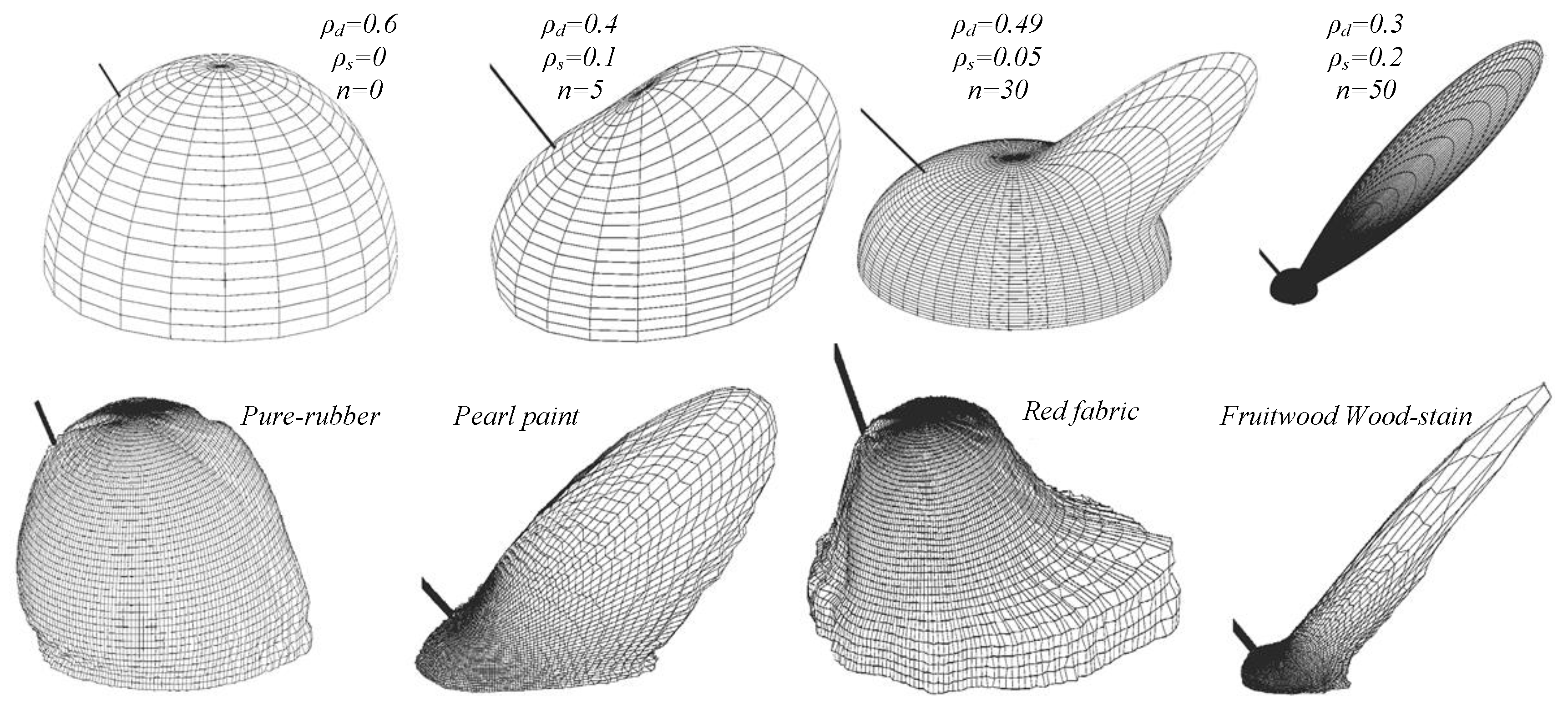
First, we briefly define Phong BRDF model to illustrate how Lambertian distribution is compared to other materials’ BRDF. Phong BRDF is given as

$$f_r=\frac{{\rho }_d}{\pi }+\frac{{\rho }_s(n+1)co{s}^n\alpha }{2\pi cos{\theta }_i}$$

(7)

${\rho }_d$ is the diffuse reflection constant, n determines the angular divergence of the lobe, and ${\rho }_s$ determines the peak value or “strength” of the lobe [23]. Figure 1 depicts BRDF distribution for different values of ${\rho }_d$, ${\rho }_s$, and n. Lambertian is a special case where ${\rho }_s$ = n = 0, leaving only the first term of Equation (7). In Figure 1, the second row shows BRDF of some real materials which approximate those in Figure 1. Rubber’s BRDF is closer to our assumption.

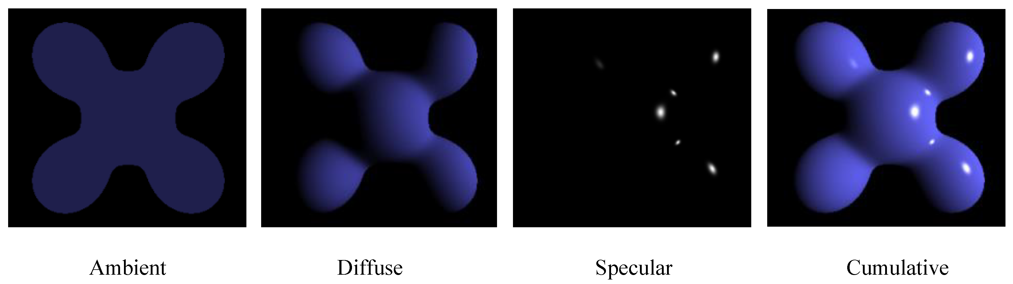
Components of reflected light based on Phong reflection model are ambient, diffuse, and specular radiance, as shown in Figure 2. Ambient reflection is both in shadowed and non-shadowed regions [13]. Diffuse (Lambertian) is assumed in this work; therefore, the specular component is the actual source of error, $e_1$, of Equation (4). Ref. [13] assumes that the specular reflection can be ignored for most urban and rural areas because these images are usually matte; we also maintain this assumption in this work.

2.1.2. Sky-View Factor Error

3-D geometry in the scene tends to cause visual occlusion to the sky-view Line of Sight (LoS). Sky-view LoS is quantified as a sky-view factor and normalized between zero and one, where zero is complete occlusion and one is clear sky-view [27]. This occlusion is one of the causes of shadow casting (apart from clouds, partial solar eclipse, etc.). Therefore, the presence of this error in the estimation would enhance the discrimination between shadowed and non-shadowed regions; hence it facilitates detection of variable illumination.

2.2. Proposed Radiative Transfer Model-Based General Relationship between Variably Illuminated Regions

ELM represents the at-sensor radiance from in-scene white and black calibration panels. Radiance reflected from the white panel $L_w$ and black panel $L_b$ is deduced from Equation (6) and shown in Equations (8) and (9), respectively.

$$L_w=L_p+\frac{\tau E_g\left(0\right)/\pi }{1-s\rho }$$

(8)

$$L_b=L_p$$

(9)

In Equation (8), $L_w$ radiance includes both path radiance and total ground-reflected radiance, which are the first and second terms, respectively. We introduce two parameters $\alpha$ and $\beta$ in Equation (10) that represent the total ground-reflected radiance and path radiance, respectively, and brings the convention to Equation (10), which is called the ELM equation.

$$\rho =\alpha Ls+\beta$$

(10)

where $\alpha$ and $\beta$ are,

$$\alpha =1/(L_w-L_b)$$

(11)

$$\beta =L_b/(L_w-L_b)$$

(12)

Reflectance $\rho$ is independent of illumination conditions, and enables us to rephrase Equation (10) as Equation (13), emphasizing only parameters $\alpha$ and $\beta$.

$$\Rightarrow f(\alpha ,\beta )=Ls=\frac{\rho -\beta }{\alpha }$$

(13)

We rewrite Equation (10) for shadowed (sub-scripted S) and non-shadowed (sub-scripted NS) regions of the scene as Equations (14) and (15), respectively.

$$\rho ={\alpha }_{NS}L{s}_{NS}\left(\rho \right)+{\beta }_{NS}$$

(14)

$$\rho ={\alpha }_{S}L{s}_S\left(\rho \right)+{\beta }_S$$

(15)

Equating Equations (14) and (15) we get Equation (16).

$$\begin{array}{c}\hfill L{s}_{NS}=\frac{{\alpha }_{S}L{s}_S\left(\rho \right)+{\beta }_S-{\beta }_{NS}}{{\alpha }_{NS}}\end{array}$$

(16a)

$$\begin{array}{c}\hfill L{s}_{NS}=\frac{{\alpha }_{S}L{s}_S\left(\rho \right)+\Delta \beta }{{\alpha }_{NS}}\end{array}$$

(16b)

where $\Delta \beta ={\beta }_S-{\beta }_{NS}$. Equation (16) is rephrased as Equation (17).

$$L{s}_{NS}=\gamma L{s}_S\left(\rho \right)+\delta$$

(17)

where

$$\begin{array}{c}\hfill \gamma ={\alpha }_S/{\alpha }_{NS}\end{array}$$

(18a)

$$\begin{array}{c}\hfill \delta =\Delta \beta /{\alpha }_{NS}\end{array}$$

(18b)

Equation (17) shows $\gamma$ and $\delta$ that are two unknown parameters responsible for illumination variability between shaded and non-shaded regions. Ideally, if $\gamma$ = 1 and $\delta$ = 0, there is no variability in illumination across the scene.

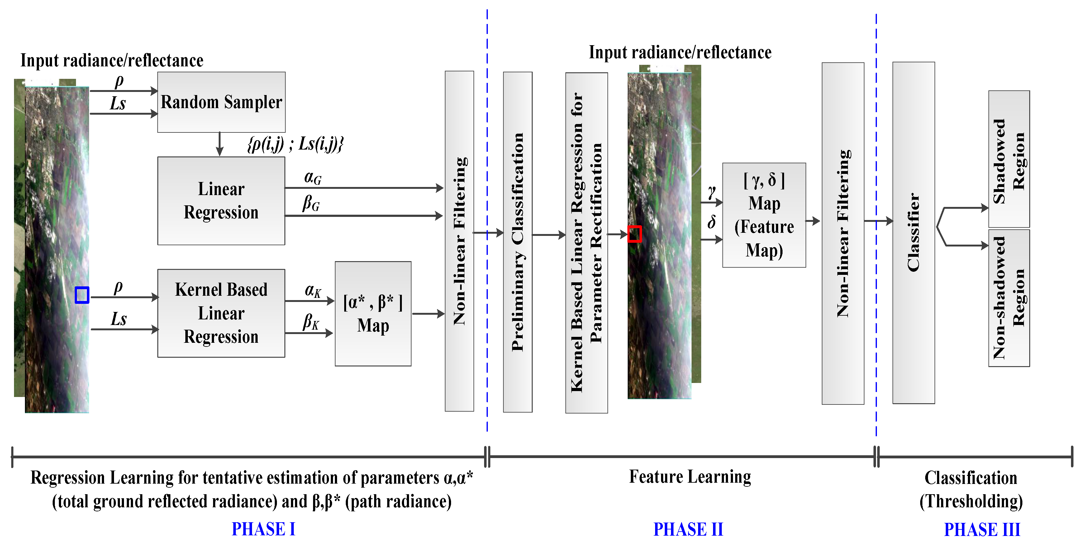
3. Proposed Multi-Layered Regression Learning Algorithm

In the previous section, a general relationship between illumination under shadowed and non-shadowed region within an HSI image is established. Estimation of discriminant parameters ${\alpha }_{NS}$,${\beta }_{NS}$,${\alpha }_S$, and ${\beta }_S$ is vital for good detection. We divide our learning algorithm into three phases: (i) regression learning; (ii) feature learning; and (iii) classification, as shown in Figure 3.

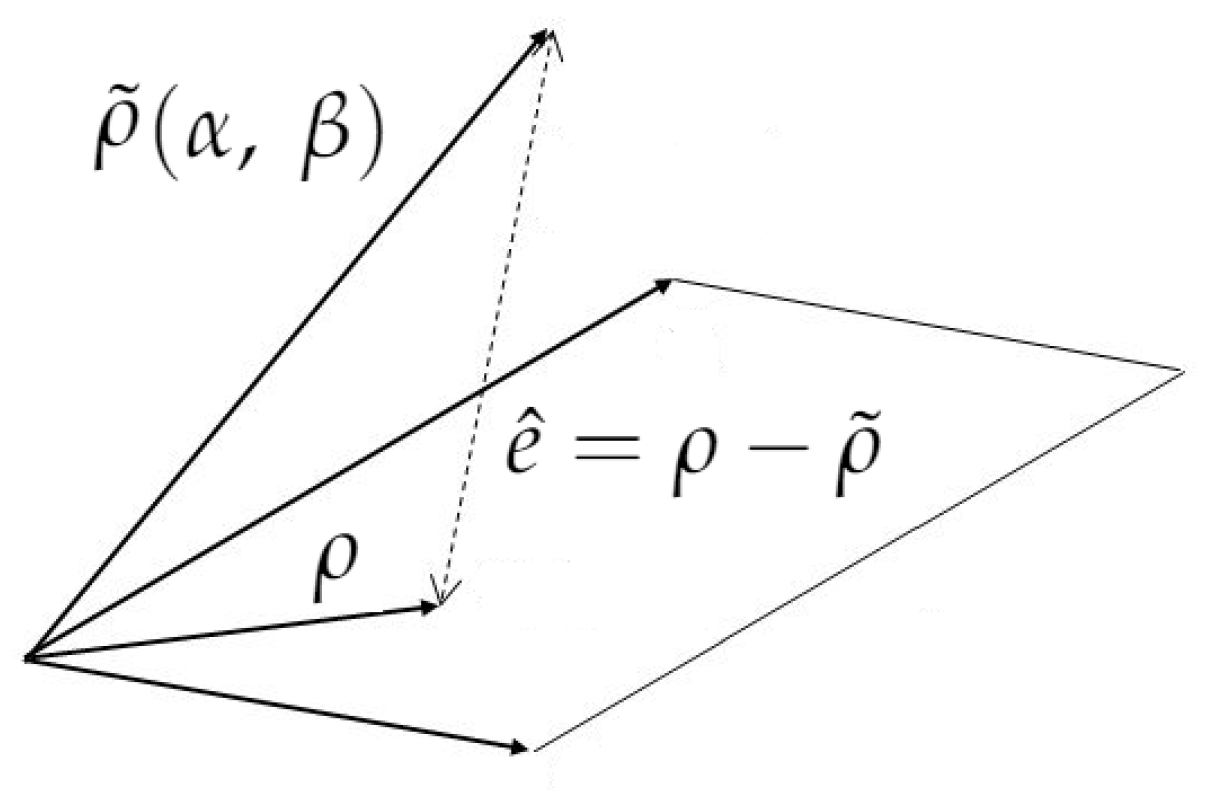
During learning, Equation (10) becomes Equation (19), where $\tilde{\rho }$ is the approximate reflectance at any given search iteration, while reflectance computed from QUAC is the reference reflectance, referred in Equation (20). Therefore, the cost function $J(\alpha ,\beta )$, to minimize is given in Equation (21), which is illustrated in Figure 4.

$$\tilde{\rho }=\alpha Ls+\beta$$

(19)

$${\rho }_{QUAC}=\rho$$

(20)

$$J(\alpha ,\beta )=\begin{array}{c}\min \\ \alpha ,\beta \end{array}\left\{\rho -\tilde{\rho }\right\}$$

(21)

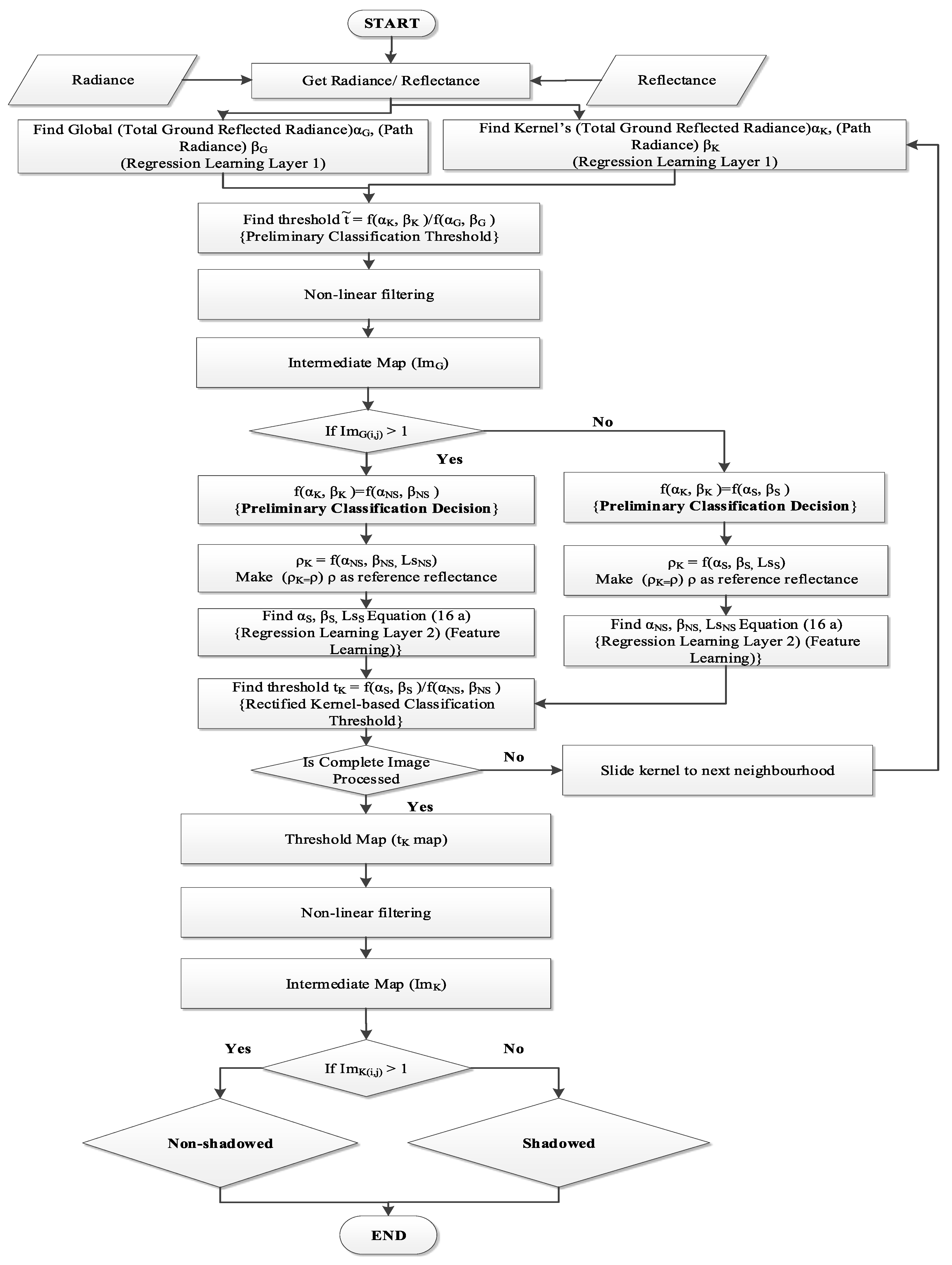
A complete flowchart of multi-layered learning is shown in Figure 5.

3.1. Regression Learning Phase

This phase is denoted as Phase I in Figure 3 and is further sub-divided into two steps:

• Global Search: Search for ${\alpha }_G$ and ${\beta }_G$ estimates of Equation (19) on random samples drawn from the whole image given a global search across the scene, as shown in Figure 3.
• Local Search: Create a 3 × 3 kernel and search for parameters ${\alpha }_K$ and ${\beta }_K$ in the kernel only i.e., localized search.

3.1.1. Global Search

Satellite/airborne images cover a larger landscape where the number of bands is more contiguous in HSI images. The high-resolution image has an immediate implication of an increase in both computing and memory requirements. To reduce these requirements, we introduced random sampling on the whole image. A random sampler selects several samples from the whole image and regression learning is performed on these samples to estimate Empirical Line Method (ELM) parameters. As the input image and samples contain neutral (both shadowed and non-shadowed) regions, parameters ${\alpha }_G$ and ${\beta }_G$ also represent the same. Equation (6) for global search case is reformulated in Equation (22).

$${\rho }_G={\alpha }_{G}L{s}_G+{\beta }_G$$

(22)

An estimate of $L_w$ and $L_b$ found in this phase is shown in Figure 6.

3.1.2. Local Search

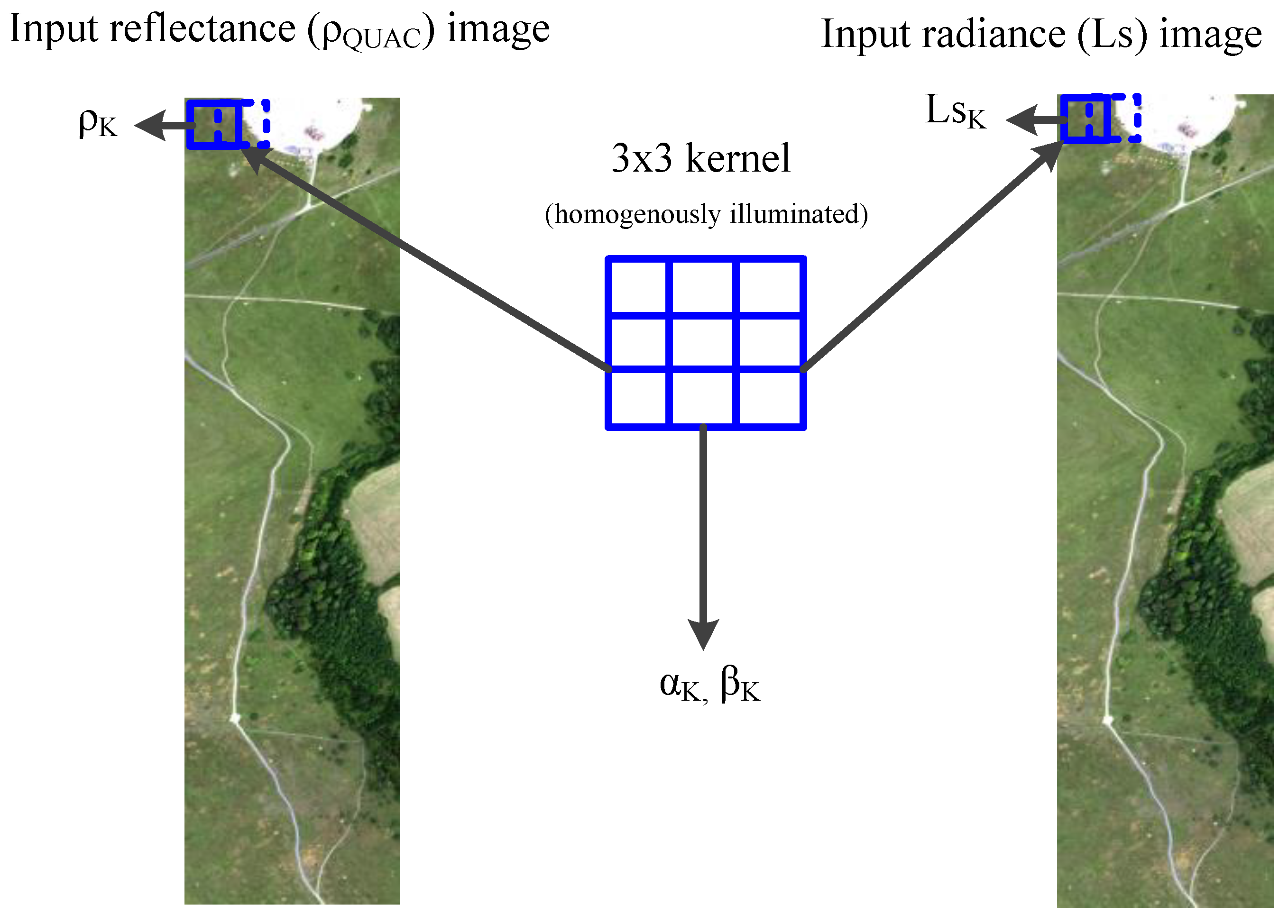
In this part of regression learning, a 3 × 3 kernel is used. A smaller kernel provides a rationale for the assumption that pixels under the kernel are homogeneously illuminated. Correctness of this assumption is further reinforced for high-resolution images that possess lower ground-sampling distance (GSD). Due to learning on a sliding kernel, this search is more time-consuming than the global one. Outputs from this step are parameter (${\alpha }_K$,${\beta }_K$) maps. An estimate of $L{w}_K$ and $L{b}_K$ for 465.611 nm is shown in Figure 7. In this case, we reformulate Equation (6) as Equation (23). Figure 8 shows the sliding kernel, and it is input and output parameters.

$${\rho }_K={\alpha }_{K}L{s}_K+{\beta }_K$$

(23)

3.2. Feature-Learning Phase

In the previous phase, we have found both global and local parameters, although we assume that since a smaller kernel has homogeneous illumination it is yet to be ascertained whether it is shadowed or non-shadowed. This phase will establish the discriminant function, first for tentative and then for the final classification. Components of feature-learning phase in Figure 3 are described in the subsequent sections.

3.2.1. Preliminary Classification

Global radiance $L{s}_G$ is estimated by inclusion of both shadowed and non-shadowed regions. $L{s}_K$ is however assumed to be either of them. A global and local version of Equation (13) is given as

$$\begin{array}{c}\hfill f({\alpha }_K,{\beta }_K)=L{s}_K=\frac{{\rho }_K-{\beta }_K}{{\alpha }_K}\end{array}$$

(24a)

$$\begin{array}{c}\hfill f({\alpha }_G,{\beta }_G)=L{s}_G=\frac{{\rho }_G-{\beta }_G}{{\alpha }_G}\end{array}$$

(24b)

In this phase, a ratio between f(${\alpha }_K$,${\beta }_K$) and f(${\alpha }_G$,${\beta }_G$) is calculated by Equation (25), which yields approximate threshold $\tilde{t}$.

$$g({\alpha }_G,{\beta }_G,{\alpha }_K,{\beta }_K)=\frac{f({\alpha }_K,{\beta }_K)}{f({\alpha }_G,{\beta }_G)}=\tilde{t}$$

(25)

$$\begin{array}{c}\hfill \tilde{t}=\left\{\begin{array}{cccc}>1& ,& f({\alpha }_K,{\beta }_K)=f({\alpha }_{NS},{\beta }_{NS}),& (\mathrm{Non}-\mathrm{shadowed})\\ <1& ,& f({\alpha }_K,{\beta }_K)=f({\alpha }_S,{\beta }_S),& \left(\mathrm{Shadowed}\right)\end{array}\right.\end{array}$$

(26)

The kernel region is assigned a shadow or non-shadow label based on Equation (26). If the value of t is greater than one, then the region under the kernel is more likely to be non-shadowed than otherwise. The above is under the intuitive assumption that the scene has more non-shadowed regions than shadowed ones. This provides a preliminary classification as shown in Figure 3 and Figure 5, and leads us to either $(L{s}_{NS}$,${\alpha }_{NS}$,${\beta }_{NS})$ or $(L{s}_S$,${\alpha }_S$,${\beta }_S)$ of Equation (16a), as per our assumption. The selection of either of these parameter sets is shown as two potential flows in Figure 5.

In practice, $\tilde{t}$ is noisy data across the optical spectrum. Therefore, non-linear filtering is applied to it for smoothing and creating an intermediate map. As filtering is applied on both global and kernel thresholds $\tilde{t}$ and $t_K$, respectively, it is discussed later in Section 3.3.

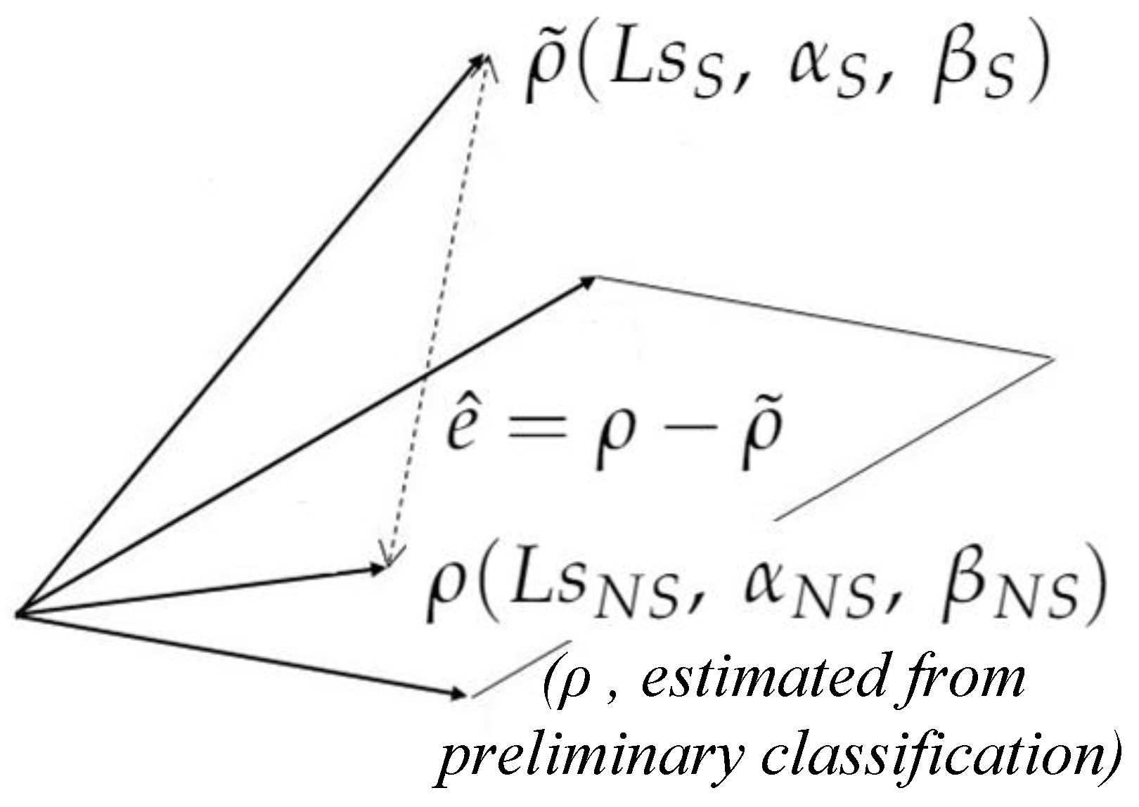
3.2.2. Regression Learning for Parameter Rectification

To create a more reliable discriminant threshold function than that of Equation (26), we need to establish a relationship between our processed parameters to bring it in the shape of Equation (16). Global and local processing has provided us with a mathematical basis for tentative classification, which is plausible under the laws of physics. We suppose that the kernel region is labelled, by preliminary classification, as non-shadowed which implies that we found $(L{s}_{NS}$,${\alpha }_{NS}$,${\beta }_{NS})$; however $(L{s}_S$,${\alpha }_S$,${\beta }_S)$ of Equation (16a) are yet to be determined for the region under the kernel. We rewrite Equation (16a), for convenience.

$$L{s}_{NS}=\frac{{\alpha }_{S}L{s}_S\left(\rho \right)+{\beta }_S-{\beta }_{NS}}{{\alpha }_{NS}}$$

(27)

$L{s}_S$,${\alpha }_S$,${\beta }_S$ are determined by another layer of regression learning. The cost function $Q(L{s}_S,{\alpha }_S,{\beta }_S)$, to minimize is given in Equation (21), which is illustrated in Figure 9.

$$\tilde{\rho }=\alpha L{s}_S+{\beta }_S$$

(28)

$$\rho ={\alpha }_{NS}L{s}_{NS}+{\beta }_{NS}$$

(29)

$$Q(L{s}_S,{\alpha }_S,{\beta }_S)=\begin{array}{c}\min \\ L{s}_S,{\alpha }_S,{\beta }_S\end{array}\left\{\rho -\tilde{\rho }\right\}$$

(30)

This learning is performed by Algorithm 1. After this learning phase, we estimated all unknown parameters of Equation (27), therefore we may rewrite Equation (25) as Equations (32) and (31). Please note that this equation is only for the kernel region, which has the same reflectance $\rho$ and has shadow and non-shadow parameters instead of global and local.

Algorithm 1 Gradient-descent algorithm for global/kernel-based search

1: Let HSI Radiance Image be “L” with “s” samples and “b” bands, and its reflectance estimated by Run QUAC to find reflectance R 2: Assign outputs $L_w$ and $L_b$ as two zeros vector of “b” 3: Let stepSize be 0.01 with a decay of 0.995 4: while ($\Delta L_w\le$ $1\times {10}^{-10}$ and $\Delta L_b\le$ 1 $\times {10}^{-10}$) do 5:     Select 2 pixels at random 6:     Estimate $\delta L_w$ and $\delta L_b$ for selected pixels by ELM equation 7:     $L_w$ = (1 − stepSize) $\times L_w$ + stepSize $\times \delta L_w$ 8:     $L_b$ = (1 − stepSize) $\times L_b$ + stepSize $\times \delta L_b$ 9:     stepSize = stepSize × decay

It is extremely important to note that if preliminary classification finds (${\alpha }_K$,${\beta }_K$) = (${\alpha }_{NS}$,${\beta }_{NS}$) then t takes the form of Equation (31). If it finds (${\alpha }_K$,${\beta }_K$) = (${\alpha }_S$,${\beta }_S$) then t takes the form of Equation (32).

$$g({\alpha }_{NS},{\beta }_{NS},{\alpha }_S,{\beta }_S)=\frac{f({\alpha }_{NS},{\beta }_{NS})}{f({\alpha }_S,{\beta }_S)}=t$$

(31)

$$g({\alpha }_S,{\beta }_S,{\alpha }_{NS},{\beta }_{NS})=\frac{f({\alpha }_S,{\beta }_S)}{f({\alpha }_{NS},{\beta }_{NS})}=t$$

(32)

Replacing both numerator and denominator of Equations (31) and (32) by right-hand side of Equation (13) in their respective form, we get Equations (33) and (34).

$$t=\frac{{\alpha }_{NS}(\rho -{\beta }_S)}{{\alpha }_S(\rho -{\beta }_{NS})}$$

(33)

$$t=\frac{{\alpha }_S(\rho -{\beta }_{NS})}{{\alpha }_{NS}(\rho -{\beta }_S)}$$

(34)

Threshold t is a better estimate than $\tilde{t}$, because both parameters are computed for the region under the kernel. This process is termed as rectification in Figure 3 and Figure 5. When the kernel slides through the image, it estimates t at each iteration. On completion, it creates an intermediate map for the whole image. As we discussed in Section 3.2.1, both $\tilde{t}$ and t are computed for all bands of HSI image and tend to get very noisy at some bands. This problem is tackled by filtering, which is covered in Section 3.3.

3.3. Filtering

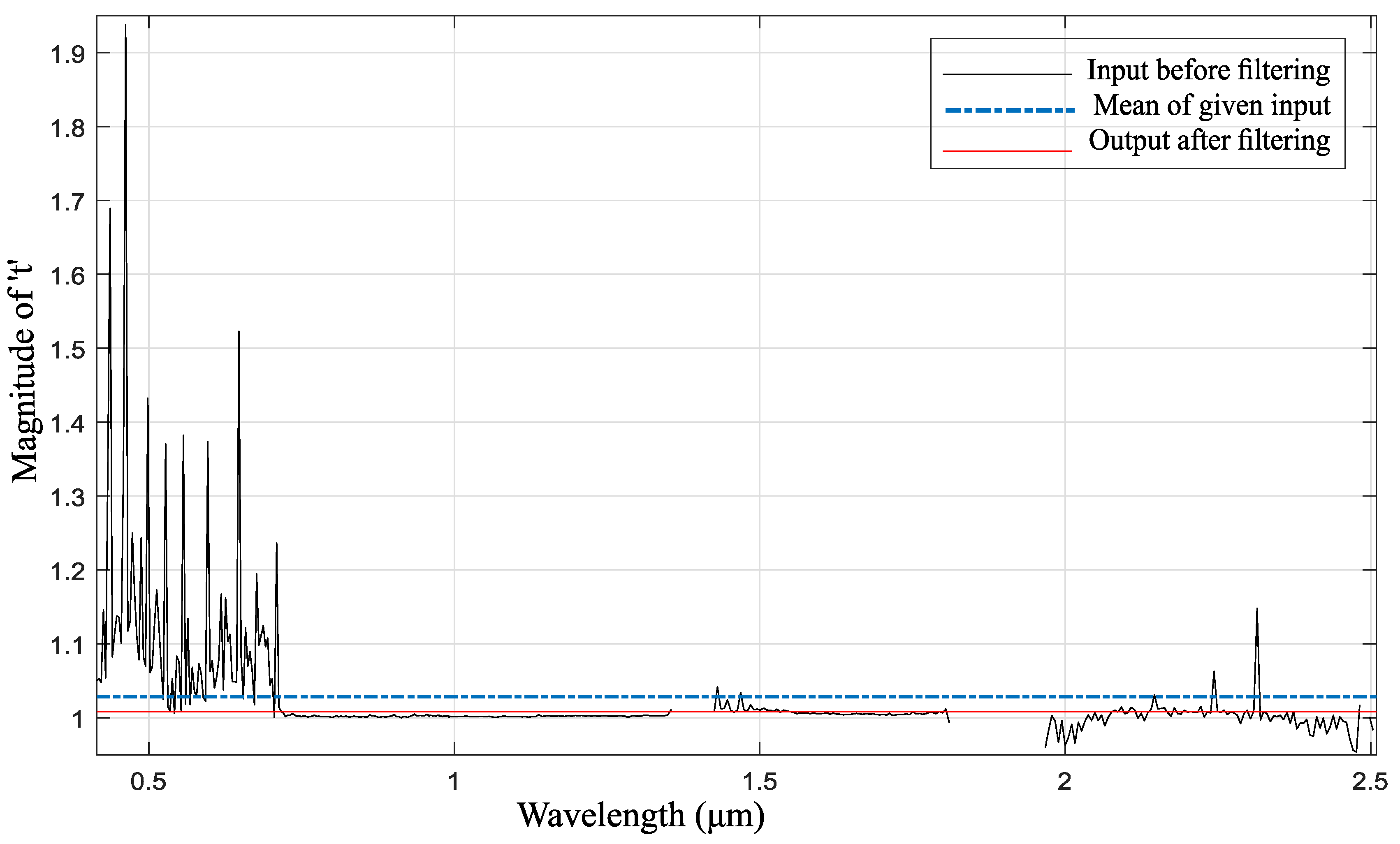
Filtering is a supplementary but vital step for the performance of detection. This is the third and final layer of regression learning. Here we estimate an activation function for a non-linear filter based on Equation (35a). The cost function $J(x,t)$ finds the value of threshold scalar x which maximizes $h(x,t)$. The subscript k shows the band number of the HSI image with B bands. Threshold t is estimated from Equations (33) and (34) and $\tilde{t}$ is found from (25), respectively. We applied this filter on our test dataset which reduces noise, as shown in Figure 10.

$$\begin{array}{c}\hfill h(x,t)=\sum _{k=1}^B{e}^{-(x-t_k)}\end{array}$$

(35a)

$$\begin{array}{c}\hfill J(x,t)=\begin{array}{c}\max \\ x\end{array}\left\{h(x,t)\right\}\end{array}$$

(35b)

The gradient-descent algorithm finds x in pseudo-code presented in Algorithm 2. Figure 10 shows output after filtering. Intermediate maps are created after the filtering process.

Algorithm 2 Gradient-descent algorithm to estimate h(x, t)

1: For an n-dimensional input ‘t’ and ‘M’ be the maximum number of iterations 2: Let the initial value of ‘x’ be mean(t) 3: Let output $h_x$ be h(x, t) 4: Let stepSize be 0.01 with a decay of 0.995 5: fori = 1 to Mdo 6:     $h_d$ = h((x-stepSize), t) 7:     $h_i$ = h((x+stepSize), t) 8:     if $h_x<h_d$ then 9:         $h_x=h_d$ 10:         x = x − stepSize 11:     if $h_x<h_i$ then 12:         $h_x=h_i$ 13:         x = x + stepSize 14:     stepSize = stepSize × decay

3.4. Classification

The threshold map generated by Feature learning and filtering represents multiple levels of illumination. Therefore, we may generate a binary or multi-label classification from this intermediate map.

3.4.1. Binary Map

To create a binary map, our approach is similar to Equation (26) threshold function, shown in Equation (36) as:

$$\begin{array}{c}\hfill t=\left\{\begin{array}{ccc}>1\hfill & ,\hfill & (\mathrm{Non}-\mathrm{shadowed})\hfill \\ <1\hfill & ,\hfill & \left(\mathrm{Shadowed}\right)\hfill \end{array}\right.\end{array}$$

(36)

Figure 7b,c show the binary map for Selene HSI dataset using 10 × 10 and 3 × 3 kernel sizes, respectively.

3.4.2. Multi-Label Classification

In practice, any decrease in radiance caused by shadows may include soft and hard shadows, depending on the amount of direct radiance blockage and scattering, which causes multi-level illumination. In order to accommodate this case when a user-defined threshold is also not a priori, dual marching squares algorithm [28] is used to automate the process. By employing this algorithm, multiple levels of illumination are separated in different contour levels, as covered in Section 5.1.3. In this algorithm, one may define several levels to generate the contour map accordingly.

4. Experimental and Validation Data

4.1. Experimental Data

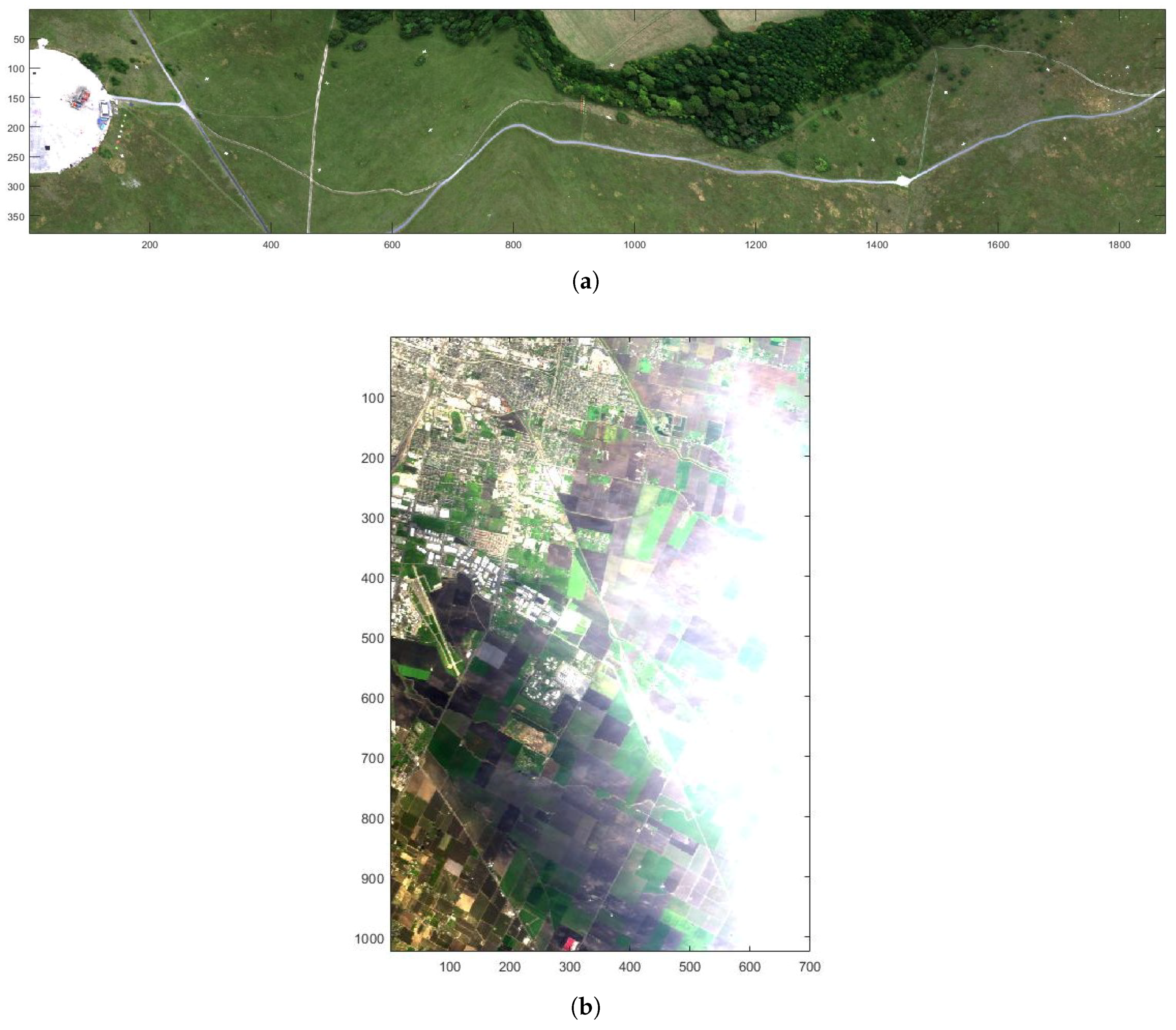
For experimental validation, we have used two real images. Our algorithm is tested on the Selene SCIH23 dataset [29] which was acquired by the Defence Science and Technology Laboratory (DSTL) covering 0.4 to 2.5 μm. It is a registered image which is separately taken from HySpex VNIR-1600 (160 bands) and SWIR-384 (288 bands) sensors mounted on the same airborne platform. This scene was acquired near Salisbury, UK, on 12 August 2014 BST 13:00:04. The registered image has a GSD of 70 × 70 cm, QUAC was applied using ENVI software for atmospheric compensation. The second image is taken from AVIRIS (224 bands), covering Modesto, California (Long 121°17′45.9″ N Lat 37°56′44.37″ W to 121°04′50.31″ N 37°51′55.67″ W) on 10 February 2015 BST 22:00:04. The latter is publicly available from https://aviris.jpl.nasa.gov/. RGB images of Selene and Modesto scenes are shown in Figure 11a,b, respectively.

4.2. Validation Data

The Selene SCIH23 scene’s terrain was mapped with a high-resolution LIDAR to create a contour-based DSM of the scene. This DSM is used in a ray-tracer to generate a shadow map, which is termed as ground truth for Selene results. Modesto does not have DSM data available. Therefore, classification performance is tested on visual perception only.

5. Results and Validation

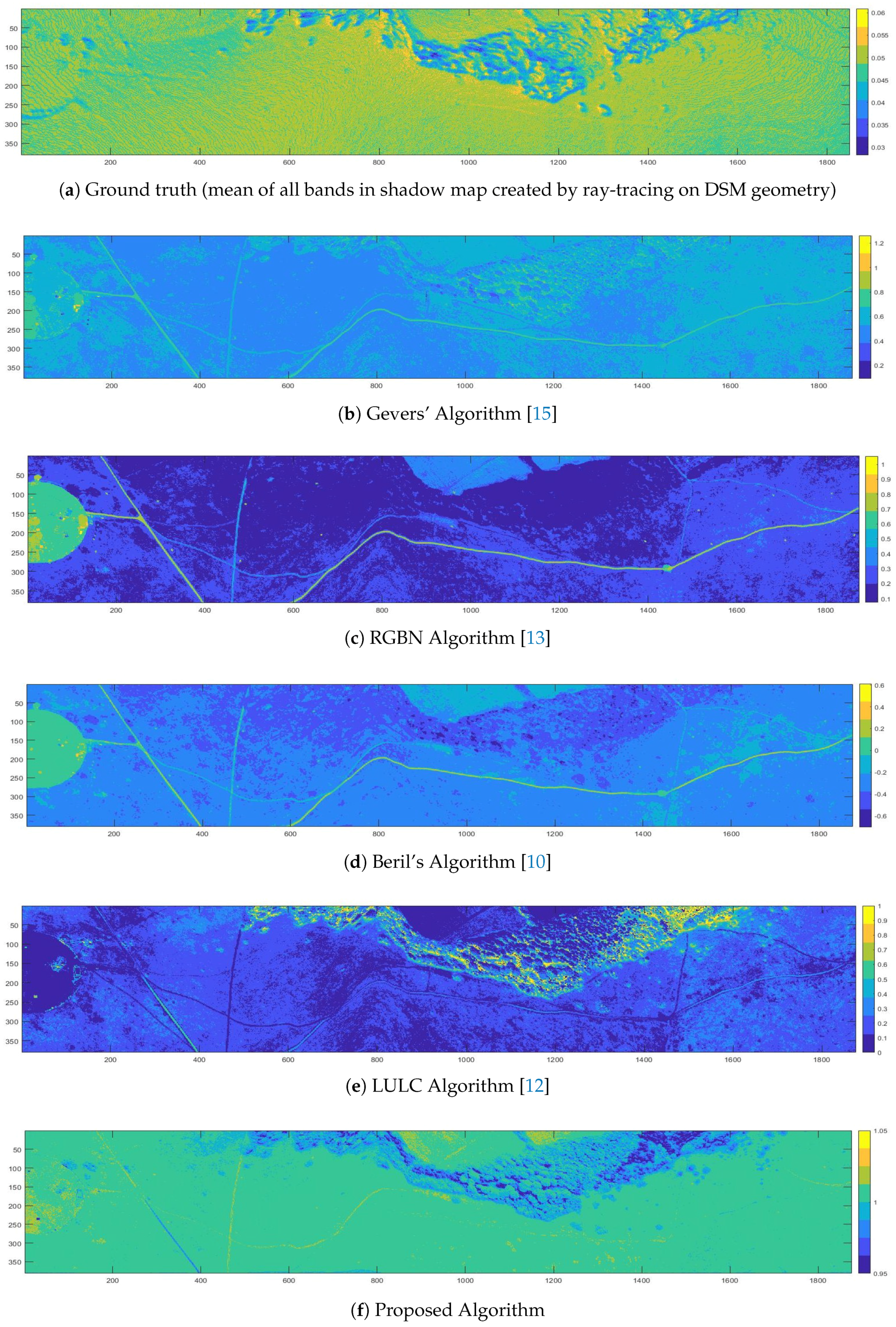
In this section, we will present results of the Selene and Modesto scenes. Construction of GT for the Selene scene enables us to provide a more quantitative validation for it by means of confusion matrix, while for Modesto, it is more qualitative and evaluated visually. For comparative analysis, we have considered both classical methods exploiting descriptor-based shadow detection from RGB input, as in Gevers [15], and Beril [10] (see [30] for source code), and methods that take in multispectral radiance input, as in RGBN [13] requiring RGB and a single NIR band, and false-color shadow detection method, LULC [12] (see [31] for source code), requiring five input bands within 0.3 μm to 2.5 μm.

5.1. Selene Scene

Firstly, the algorithm is executed on the Selene SCI H23 scene for both global and local search sub-phases of the regression learning phase. This scene has several white and black calibration panels planted, providing us with a GT for comparison of estimated global $L_w$ and $L_b$.

5.1.1. Result of Regression Learning on Whole Image (Global Search)

The comparative result for global search sub-phase is shown in Figure 6. The Normalized Root Mean Square Error (NRMSE) for $L_w$ is 20.62%, which shows that the algorithm can reconstruct the white panel with substantial accuracy. The deviation in the blue region shows under-estimation of scattering/sky radiance, while lower magnitude in NIR is due to over-estimation of the adjacency effect, which is primarily caused by the abundance of vegetation in the background scene. The NRMSE for $L_b$ is 76.66%, which is higher than $L_w$, it shows that the adjacency effect is over-estimated, hence the estimated black panel looks similar to the vegetating signature. These errors were incurred due to QUAC reflectance, which is the reference for calculating the $L_w$ and $L_b$ in our algorithm.

5.1.2. Results of Kernel-Based Regression Learning (Local Search)

Figure 7a shows the GT shadow map generated from ray-tracer on DSM. Figure 7b,c show results of local search sub-phase. In the case of former, the algorithm was run with a coarse kernel (10 × 10) and the latter with a fine (3 × 3) kernel. Better separation of shadowed and non-shadowed regions is visible with 3 × 3 kernel compared to its coarse counterpart.

In case of the fine kernel, shadows due to bumps on the terrain are also captured which seems to be missing from the coarser one.

5.1.3. Results of Classification

• Intermediate and Binary maps
  Algorithms adopted for comparative analysis create an intermediate map and apply manual threshold as suggested by respective authors. We propose a cut-off value of 1 due to the ratio between shadow and non-shadow radiance. Intermediate maps of all algorithms for the Selene scene are shown in Figure 12. After applying respective threshold values, we get binary classification maps for the Selene scene as shown in Figure 13. The Selene scene has shadowed regions near trees and concrete fields. The concrete field has some buildings that are casting shadows there. The grass field has a few bumps and has some stand-alone tree distribution along the track.
  The binary map for the Selene scene GT is constructed by applying a threshold on the DSM contour data. Similarly, the binary map of all competitive algorithms is also constructed. A confusion matrix of each algorithm against GT is tabulated, which is shown in

  Table 1. Evaluation of accuracy of the methods in Figure 13 where true positive and true negative is successful detection of shadowed and non-shadowed areas respectively compared with ground truth (GT) DSM simulated map, and ”n” represent cardinality.

  Method	$\frac{\mathit{n}\left(\mathbf{True}\mathbf{Positive}\right)}{\mathit{n}\left(\mathbf{GT}\mathbf{Shadow}\right)}\times \mathbf{100}$	$\frac{\mathit{n}\left(\mathbf{False}\mathbf{Positive}\right)}{\mathit{n}\left(\mathbf{GT}\mathbf{Shadow}\right)}\times \mathbf{100}$	$\frac{\mathit{n}\left(\mathbf{True}\mathbf{Negative}\right)}{\mathit{n}\left(\mathbf{GT}\mathbf{Non}-\mathbf{Shadow}\right)}\times \mathbf{100}$	$\frac{\mathit{n}\left(\mathbf{False}\mathbf{Negative}\right)}{\mathit{n}\left(\mathbf{GT}\mathbf{Non}-\mathbf{Shadow}\right)}\times \mathbf{100}$
  Gevers	28.9013%	112.1443%	89.7015%	5.5403%
  RGBN	27.1437%	108.9442%	89.9558%	5.6801%
  Beril	0%	0.2418%	98.5948%	7.8373%
  LULC	39.5298%	72.6458%	92.8406%	4.6957%
  Proposed	40.4656%	64.4731%	93.4901%	4.6213%

  The average of true positive and true negative of Gevers, RGBN, Beril, LULC, and the proposed method are 59.3014%, 58.5497%, 49.2974%, 66.1852%, and 66.9779% respectively.

  . Because the area of the non-shadowed region is significantly larger, covering 92.6377% of the scene, compared to the shadowed region, covering 7.3623% as estimated from the DSM binary map, we divide by the cardinality in the table to minimize bias in overall percentage accuracy.
• Multi-level Classification
  The DSM-based GT shadow map in Figure 14 shows contours; therefore, the shadow map from our algorithm is also converted to contour levels. Both datasets are generated to have four contour levels and are compared one to one. The first layer has the lowest accuracy, with 53.09%, which is in the non-shadowed region. The second layer has a partial shadowed region; a raise in the accuracy is observed in this case. As we step further to Layer 3 and Layer 4, which appear to capture shadowed regions, the accuracy increased to 69.6% and 88.2%, respectively.

5.2. Modesto Scene

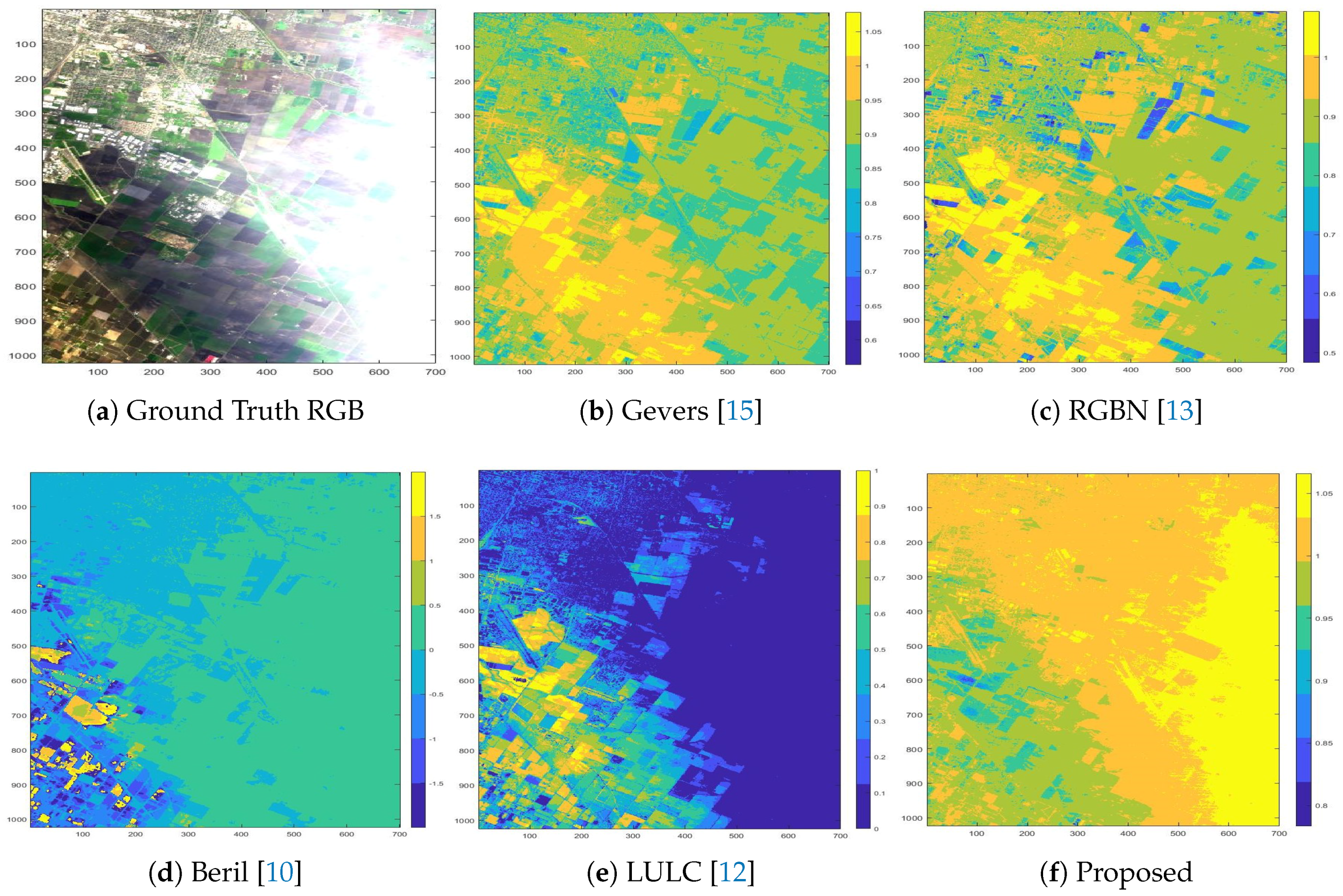
The Modesto scene does not have DSM data. Therefore, ground truth for this scene is not available. The evaluation, in this case, is rather qualitative, based on visual perception. Intermediate maps of all algorithms of interest for the Modesto scene are shown in Figure 15. Their binary counterparts are in Figure 16. The proposed algorithm appears to classify the scene into three regions: (i) with clouds, (ii) with shadows, and (iii) the lit ground region. After the threshold is applied to the intermediate map, the scene is classified into shadowed and non-shadowed regions, as shown in Figure 16.

6. Discussion

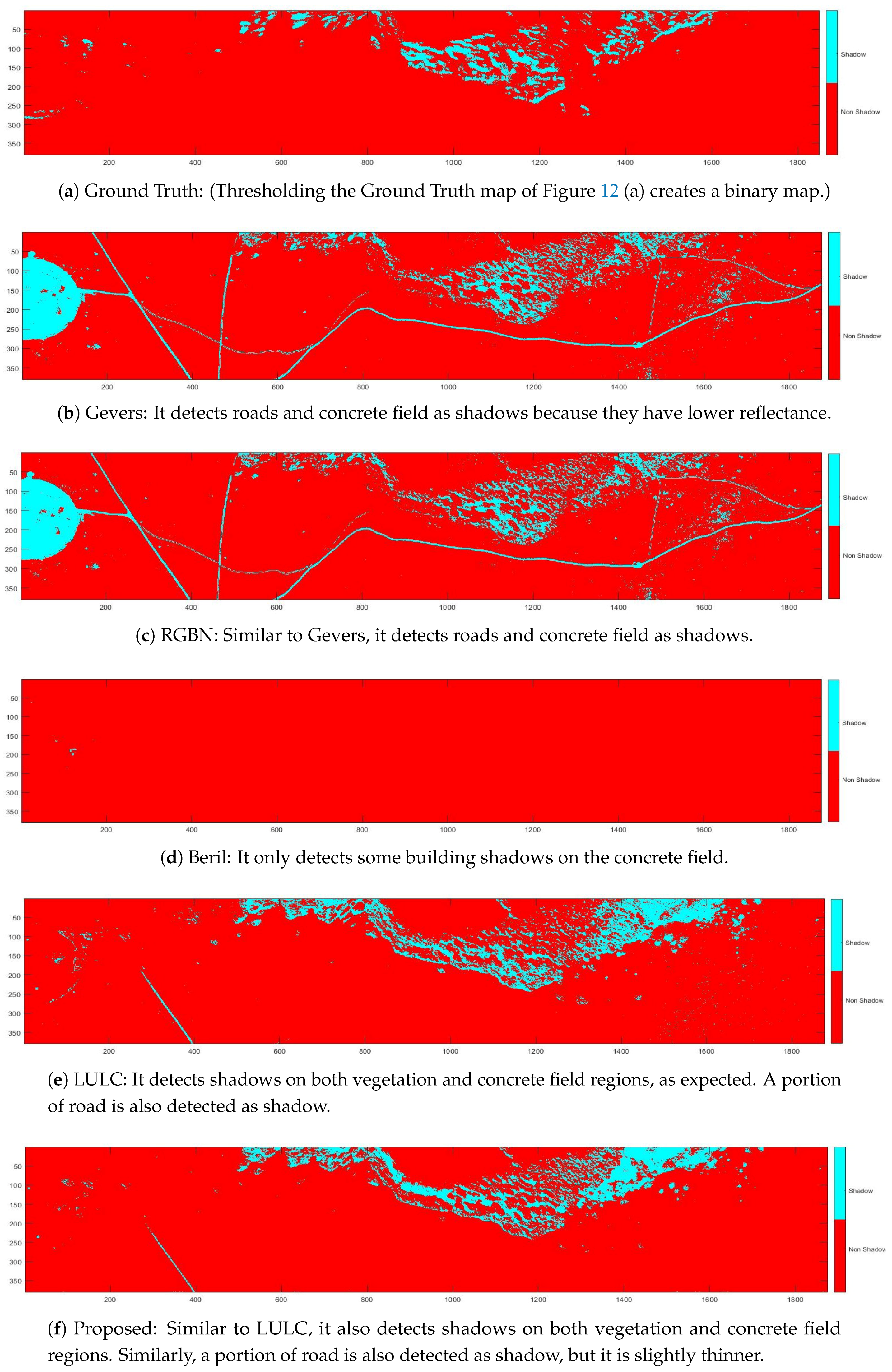
The Selene scene GT shadow map enables us to quantify the results of comparative algorithms in context. The proposed algorithm is shown to have 40.46% true positive, i.e., correct detection of a shadow region compared to other counterparts. In this case, the LULC algorithm is marginally inferior to our algorithm, yielding 39.52%. Beril, RGBN, and Gevers reach 0%, 27.14%, and 28.90%, respectively. In terms of false positive, i.e., detecting non-shadow as a shadow, our algorithm continues to perform better than other algorithms, reaching 64% compared to 72.64% of LULC, 112.14% of Gevers, and 108.94% of RGBN. Although Beril shows a lower value of 0.24%, it should be noted that it is the most biased performer, detecting 98% of the region as non-shadowed. Ignoring the Beril algorithm due to bias, our algorithm tops the true-negative detection as well, i.e., detecting non-shadowed region correctly. Our result is 93.49% compared to 92.8%, 89.9%, and 89.7% of LULC, RGBN, and Gevers algorithms, respectively. Finally, our algorithm is also the best performer in false negative, i.e., detecting non-shadow as a shadow, yielding only 4.62% compared 4.69%, 5.68%, and 5.54% of LULC, RGBN, and Gevers algorithms, respectively. We conclude that LULC is marginally inferior to our algorithm while others are completely outperformed.

For the Modesto scene, a qualitative evaluation was performed, and it looks like our algorithm performed reasonably well in this dataset.

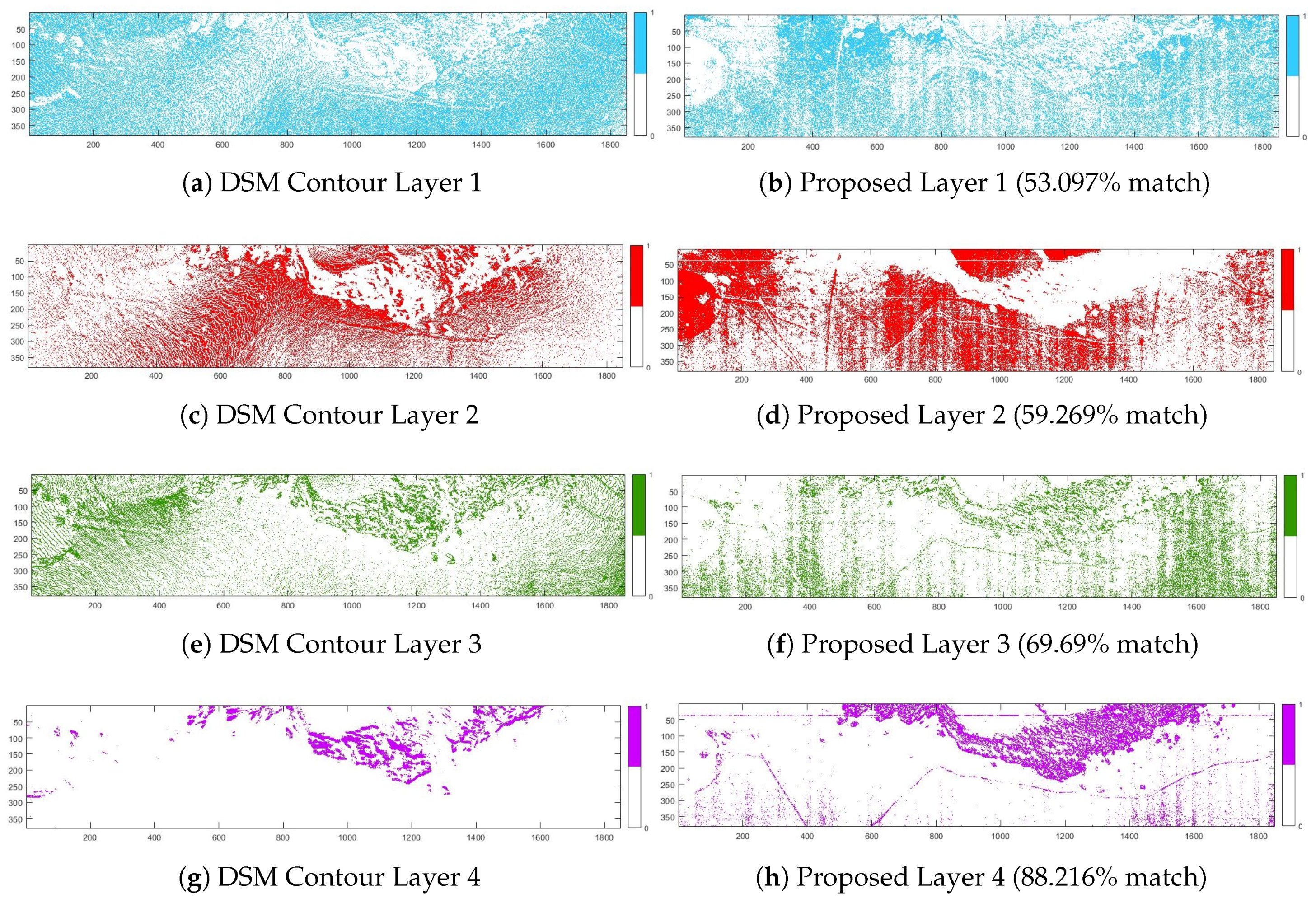
In the case of multi-label classification of the Selene scene, GT and our algorithm intermediate maps were divided into four contour levels. Firstly, we can demonstrate the ability of this proposed approach to estimate shadows without any manual input from the user. Moreover, as Figure 14 manifests, the accuracy of the proposed method increased on contour levels from non-shadow top layer with 53% to shadowed bottom layer with 88% accuracy.

We believe that this direction of RT-based methods for shadow-map detection is more faithful than other intensity and band index-based methods. Moreover, it can be conveniently extended to shadow compensation work.

References

- Arvidson, T.; Gasch, J.; Goward, S.N. Landsat 7’s long-term acquisition plan—An innovative approach to building a global imagery archive. Remote Sens. Environ. 2001, 78, 13–26. [Google Scholar] [CrossRef]
- Irish, R.R. Landsat 7 Automatic Cloud Cover Assessment; International Society for Optics and Photonics: Orlando, FL, USA, 2000; pp. 348–355. [Google Scholar]
- Zhu, Z.; Woodcock, C.E. Object-based cloud and cloud shadow detection in Landsat imagery. Remote Sens. Environ. 2012, 118, 83–94. [Google Scholar] [CrossRef]
- Zhang, H.; Sun, K.; Wenzhuo, L. Object-Oriented Shadow Detection and Removal From Urban High-Resolution Remote Sensing Images. IEEE Trans. Geosci. Remote Sens. 2014, 52, 6972–6982. [Google Scholar] [CrossRef]
- Salvador, E.; Cavallaro, A.; Ebrahimi, T. Shadow identification and classification using invariant color models. In Proceedings of the 2001 IEEE International Conference on Acoustics, Speech, and Signal Processing (Cat. No. 01CH37221), Salt Lake City, UT, USA, 7–11 May 2001; Volume 3, pp. 1545–1548. [Google Scholar] [CrossRef]
- Liu, X.; Hou, Z.; Shi, Z.; Bo, Y.; Cheng, J. A shadow identification method using vegetation indices derived from hyperspectral data. Int. J. Remote Sens. 2017, 38, 5357–5373. [Google Scholar] [CrossRef]
- Imai, N.N.; Tommaselli, A.M.G.; Berveglieri, A.; Moriya, E.A.S. Shadow Detection in Hyperspectral Images Acquired by UAV. ISPRS-Int. Arch. Photogramm. Remote Sens. Spat. Inf. Sci. 2019, 4213, 371–377. [Google Scholar] [CrossRef]
- Tolt, G.; Shimoni, M.; Ahlberg, J. A shadow detection method for remote sensing images using VHR hyperspectral and LIDAR data. In Proceedings of the 2011 IEEE International Geoscience and Remote Sensing Symposium, Vancouver, BC, Canada, 24–29 July 2011; pp. 4423–4426. [Google Scholar] [CrossRef]
- Hartzell, P.; Glennie, C.; Khan, S. Terrestrial Hyperspectral Image Shadow Restoration through Lidar Fusion. Remote Sens. 2017, 9, 421. [Google Scholar] [CrossRef]
- Sirmacek, B.; Unsalan, C. Damaged building detection in aerial images using shadow Information. In Proceedings of the 2009 4th International Conference on Recent Advances in Space Technologies, Istanbul, Turkey, 11–13 June 2009; pp. 249–252. [Google Scholar] [CrossRef]
- Otsu, N. A Threshold Selection Method from Gray-Level Histograms. IEEE Trans. Syst. Man Cybern. 1979, 9, 62–66. [Google Scholar] [CrossRef]
- Teke, M.; Başeski, E.; Ok, A.Ö.; Yüksel, B.; Şenaras, Ç. Multi-spectral False Color Shadow Detection. In Photogrammetric Image Analysis; Stilla, U., Rottensteiner, F., Mayer, H., Jutzi, B., Butenuth, M., Eds.; Springer: Berlin/Heidelberg, German, 2011; pp. 109–119. [Google Scholar]
- Sevim, H.D.; Çetin, Y.Y.; Başkurt, D.Ö. A novel method to detect shadows on multispectral images. Proc. SPIE 2016, 10004, 100040A. [Google Scholar] [CrossRef]
- Sarabandi, P.; Yamazaki, F.; Matsuoka, M.; Kiremidjian, A. Shadow detection and radiometric restoration in satellite high resolution images. In Proceedings of the 2004 IEEE International Geoscience and Remote Sensing Symposium (IGARSS 2004), Anchorage, AK, USA, 20–24 September 2004; Volume 6, pp. 3744–3747. [Google Scholar] [CrossRef]
- Smeulders, A.W.M.; Bagdanov, A.D. Color Feature Detection. In Color in Computer Vision; John Wiley & Sons, Inc.: Hoboken, NJ, USA, 2012; Chapter 13; pp. 187–220. [Google Scholar] [CrossRef]
- Bernstein, L.S.; Jin, X.; Gregor, B.; Adler-Golden, S.M. Quick atmospheric correction code: Algorithm description and recent upgrades. Opt. Eng. 2012, 51, 111719. [Google Scholar] [CrossRef]
- Schott, J.R. Fundamentals of Polarimetric Remote Sensing; SPIE Press: Bellingham, WA, USA, 2009. [Google Scholar] [CrossRef]
- Nicodemus, F.E. Directional Reflectance and Emissivity of an Opaque Surface. Appl. Opt. 1965, 4, 767–775. [Google Scholar] [CrossRef]
- Stamnes, K.; Tsay, S.C.; Wiscombe, W.; Jayaweera, K. Numerically stable algorithm for discrete-ordinate-method radiative transfer in multiple scattering and emitting layered media. Appl. Opt. 1988, 27, 2502–2509. [Google Scholar] [CrossRef] [PubMed]
- Tanre, D.; Herman, M.; Deschamps, P.Y. Influence of the background contribution upon space measurements of ground reflectance. Appl. Opt. 1981, 20, 3676–3684. [Google Scholar] [CrossRef] [PubMed]
- Kaufman, Y.J. The atmospheric effect on the separability of field classes measured from satellites. Remote Sens. Environ. 1985, 18, 21–34. [Google Scholar] [CrossRef]
- Richter, R.; Bachmann, M.; Dorigo, W.; Muller, A. Influence of the Adjacency Effect on Ground Reflectance Measurements. IEEE Geosci. Remote Sens. Lett. 2006, 3, 565–569. [Google Scholar] [CrossRef]
- Willers, C.J. Electro-Optical System Analysis and Design: A Radiometry Perspective; SPIE Press: Bellingham, WA, USA, 2013. [Google Scholar] [CrossRef]
- Matusik, W.; Pfister, H.; Brand, M.; McMillan, L. A Data-Driven Reflectance Model. Ph.D. Thesis, Massachusetts Institute of Technology, Cambridge, MA, USA, 2003. [Google Scholar]
- Matusik, W.; Pfister, H.; Brand, M.; McMillan, L. Mitsubishi Electric Research Laboratory BRDF Database, Version 2. 2006. Available online: https://www.merl.com/brdf/ (accessed on 5 August 2019).
- Smith, B. Illustration of the Phong Reflection Model. Wikipedia, the Free Encyclopedia. 2006. Available online: https://en.wikipedia.org/wiki/Phong_reflection_model (accessed on 19 July 2019).
- Bernard, J.; Bocher, E.; Petit, G.; Palominos, S. Sky View Factor Calculation in Urban Context: Computational Performance and Accuracy Analysis of Two Open and Free GIS Tools. Climate 2018, 6, 60. [Google Scholar] [CrossRef]
- Gong, S.; Newman, T.S. Dual Marching Squares: Description and analysis. In Proceedings of the 2016 IEEE Southwest Symposium on Image Analysis and Interpretation (SSIAI), Santa Fe, NM, USA, 6–8 March 2016; pp. 53–56. [Google Scholar] [CrossRef]
- Piper, J.; Clarke, D.; Oxford, W. A new dataset for analysis of hyperspectral target detection performance. In Proceedings of the HSI 2014, Hyperspectral Imaging and Applications Conference, Coventry, UK, 15–16 October 2014. [Google Scholar]
- Sirmacek, B. Source Code for Beril’s Algorithm. The MathWorks, Inc., 2016. Available online: https://www.mathworks.com/matlabcentral/fileexchange/56263-shadow-detection (accessed on 5 August 2019).
- Teke, M. Source code for LULC algorithm. GitHub, Inc., 2014. Available online: https://github.com/mustafateke/FalseColorShadowDetection/blob/master/False_Color_Shadow_Detection_w_LULC.m (accessed on 5 August 2019).