Targeted Adaptable Sample for Accurate and Efficient Quantile Estimation in Non-Stationary Data Streams

Abstract

The need to detect outliers or otherwise unusual data, which can be formalized as the estimation a particular quantile of a distribution, is an important problem that frequently arises in a variety of applications of pattern recognition, computer vision and signal processing. For example, our work was most proximally motivated by the practical limitations and requirements of many semi-automatic surveillance analytics systems that detect abnormalities in closed-circuit television (CCTV) footage using statistical models of low-level motion features. In this paper, we specifically address the problem of estimating the running quantile of a data stream with non-stationary stochasticity when the absolute (rather than asymptotic) memory for storing observations is severely limited. We make several major contributions: (i) we derive an important theoretical result that shows that the change in the quantile of a stream is constrained regardless of the stochastic properties of data; (ii) we describe a set of high-level design goals for an effective estimation algorithm that emerge as a consequence of our theoretical findings; (iii) we introduce a novel algorithm that implements the aforementioned design goals by retaining a sample of data values in a manner adaptive to changes in the distribution of data and progressively narrowing down its focus in the periods of quasi-stationary stochasticity; and (iv) we present a comprehensive evaluation of the proposed algorithm and compare it with the existing methods in the literature on both synthetic datasets and three large “real-world” streams acquired in the course of operation of an existing commercial surveillance system. Our results and their detailed analysis convincingly and comprehensively demonstrate that the proposed method is highly successful and vastly outperforms the existing alternatives, especially when the target quantile is high-valued and the available buffer capacity severely limited.

1. Introduction

The problem of quantile estimation is of pervasive importance across a variety of signal processing applications. It is used extensively in data mining [1], simulation modelling [2], database maintenance, risk management in finance [3,4,5], and the analysis of computer network latencies [6,7], amongst others. A particularly challenging form of the quantile estimation problem arises when the desired quantile is high-valued (i.e., close to one, corresponding to the tail of the underlying distribution) and when data need to be processed as a stream, with limited memory capacity. An illustrative example of a practical application that imposes these constraints is that of modern CCTV-based surveillance systems. In summary, as various types of low-level observations related to events in the scene of interest arrive in real time, quantiles of the corresponding statistics for time windows of different duration are needed in order to distinguish “normal” (common) events from those that are in some sense unusual and thus require human attention [8]. The amount of incoming data is extraordinarily large and the capabilities of the available hardware highly limited both in terms of storage capacity and processing power. For further detail, see Section 3.1.2.

In this paper, we describe a novel method that addresses the aforementioned problem. It is an extension of our previous work [9], and it contains the following new content (over 45% of the total content of the manuscript):

• A more detailed description of the underlying theory and the derivation of all mathematical formulae,
• New experiments (double the amount) that illustrate further the behaviour of our algorithm and its advantages over the existing methodologies and 
• More comprehensive analysis of the results and an in-depth discussion of new findings.

Previous Work

Unsurprisingly, the problem of estimating a quantile of a set has received considerable research attention, much of it in the realm of theoretical research. In particular, a substantial amount of effort has been directed towards the study of the asymptotic limits of the computational complexity of quantile estimation algorithms [10,11]. An important result emerging from this corpus of work is the proof by Munro and Paterson [11], which in summary states that the working memory requirement of any algorithm that determines the median of a set by making at most p sequential passes through the input is $\Omega \left(n^{1/p}\right)$ (i.e., asymptotically growing at least as fast as $n^{1/p}$). This implies that the exact computation of a quantile requires $\Omega \left(n\right)$ working memory. Therefore, a single-pass algorithm, required to process streaming data, will necessarily produce an estimate and not be able to guarantee the exactness of its result.

Most of the quantile estimation algorithms developed for use in practice are not single-pass algorithms and thus cannot be applied to streaming data [12]. On the other hand, many single-pass approaches focus on the exact computation of the quantile and, therefore, as explained previously, demand $O\left(n\right)$ storage space, which is clearly an unfeasible proposition in the context we consider in the present paper. Amongst the few methods described in the literature and that satisfy our constraints are the histogram-based method of Schmeiser and Deutsch [13] and the $P^2$algorithm of Jain and Chlamtac [2] (with a similar approach described by McDermott et al. [14]). Schmeiser and Deutsch maintained a preset number of bins, scaling their boundaries to cover the entire data range as needed and keeping them equidistant. Jain and Chlamtac attempted to maintain a small set of ad hoc selected key points of the data distribution, updating their values using quadratic interpolation as new data arrive. In contrast, various random sample methods, such as that described by Vitter [15] and Cormode and Muthukrishnan [16], use different sampling strategies to fill the available buffer with random data points from the stream and estimate the quantile using the distribution of values in the buffer. Lastly, the recently-proposed algorithm of Arandjelović et al. [17] employs an adaptable quasi-maximum entropy histogram; their approach is discussed further in Section 2.2.

In addition to the ad hoc elements of the previous algorithms for quantile estimation on streaming data, which itself is a sufficient cause for concern when the algorithms need to be deployed in applications that demand high robustness and well-understood failure modes, it is also important to recognize that an implicit assumption underlying these approaches is that the data are governed by a stationary stochastic process. The assumption is often invalidated in real-world applications. As we will demonstrate in Section 3, a consequence of this discrepancy between the model underlying existing algorithms and the nature of data in practice is a major deterioration in the quality of quantile estimates. Our principal aim is thus to formulate a method that can cope with non-stationary streaming data in a more robust manner.

2. Proposed Algorithm

We start this section by formalizing the notion of a quantile. This is then followed by the introduction of the key premise of our contribution and finally a description of two algorithms that exploit the underlying idea in different ways. The algorithms are evaluated on real-world data in the next section.

2.1. Quantiles

Let p be the probability density function of a real-valued random variable X. Then, the q-quantile $v_q$ of p is defined as:

$$\begin{array}{c}\hfill {\int }_{-\infty }^{v_q}p\left(x\right)dx=q.\end{array}$$

(1)

Similarly, the q-quantile of a finite set D can be defined as:

$$\begin{array}{c}\hfill \left|\{x:x\in D\mathrm{and}x\le v_q\}\right|\le q\times \left|D\right|.\end{array}$$

(2)

In other words, the q-quantile is the smallest value below which a q fraction of the total values in a set lie. The concept of a quantile is thus intimately related to the tail behaviour of a distribution.

2.2. Challenges of Non-Stochasticity

In this work, our aim is to develop a method for quantile estimation applicable not only to streams that exhibit stationary stochasticity, but also to the all-encompassing set of streams that includes those with non-stationary data. It is a straightforward consequence of potential non-stationarity that at no point in time can it be assumed that the historical distribution of data values is representative of the future distribution of the stream data. This is true regardless of how much historical data have been seen. Thus, the value of a particular quantile can change greatly and rapidly, in either direction (i.e., increase or decrease). This is illustrated on an example, extracted from a real-world dataset used for surveillance video analysis (the full data corpus is used for comprehensive evaluation of different methods in Section 3), in Figure 1. In particular, the top plot in this figure shows the variation of the ground truth 0.95-quantile, which corresponds to the data stream shown in the bottom plot. Notice that the quantile exhibits little variation over the course of approximately the first 75% of the duration of the time window (the first 190,000 data points). This corresponds to a period of little activity in the video from which the data were extracted (see Section 3 for a detailed explanation). Then, the value of the quantile increases rapidly for over an order of magnitude; this is caused by a sudden burst of activity in the surveillance video and the corresponding change in the statistical behaviour of the data.

It may appear to be the case that to be able to adapt to such unpredictable variability in input, it is necessary to maintain an approximation of the entire distribution of historical data. Indeed, this is argued in a recent work, which introduced the data-aligned maximum entropy histogram algorithm for quantile estimation from streams [17]. The method employs a histogram of a fixed length, determined by the available working memory, which adjusts bin boundary values in a manner that maximizes the entropy of the corresponding estimate of the historical data distribution.

Although it is true that the change in the value of a specific quantile may be of an arbitrary large magnitude, in this paper, we show that its specific value in a particular stream is nevertheless constrained. Succinctly put, this is a consequence of the fact that although the stream data may be considered as being drawn from a continuous probability density function (which may change with time), the information available to our algorithm inherently comprises discrete quanta: individual data points.

2.3. Constraints: Key Theoretical Results

Consider a stream of values $x_1,x_2,\dots ,x_n$. For the time being, let us assume that there are no repeated values in the stream, i.e., $\forall i,j.x_i=x_j⟹i=j$. Then, there is an indexing function $f\left(\dots \right)$ such that $x_{f_n\left(1\right)}<x_{f_n\left(2\right)}<\dots <x_{f_n\left(n\right)}$. Let $x_{q\left(n\right)}=x_{f\left(k\right)}$ be the current estimate of a particular quantile q of interest. Consider $\Delta k$, the change in k that the arrival of a new datum $x_{n+1}$ effects. By the definition given in Equation (2):

$$\begin{array}{cc}\hfill \Delta k=& \lfloor (1-q)\times (n+1)\rfloor -\lfloor (1-q)\times n\rfloor .\hfill \end{array}$$

(3)

Exploiting simple properties of the flood function then leads to the following series of inequalities and an upper bound on $\Delta k$:

$$\begin{array}{cc}\hfill \Delta k=& \lfloor (1-q)\times (n+1)\rfloor -\lfloor (1-q)\times n\rfloor \hfill \end{array}$$

(4)

$$\begin{array}{cc}\hfill \le & (1-q)\times (n+1)-\lfloor (1-q)\times n\rfloor \hfill \end{array}$$

(5)

$$\begin{array}{cc}\hfill =& (1-q)\times n-\lfloor (1-q)\times n\rfloor +(1-q)\hfill \end{array}$$

(6)

$$\begin{array}{cc}\hfill <& 1+(1-q)=2-q<2,\hfill \\ \hfill \mathrm{and}\sin \mathrm{ce}& \Delta k\mathrm{has}\mathrm{to}\mathrm{be}\mathrm{an}\mathrm{integer}:\hfill \end{array}$$

(7)

$$\begin{array}{cc}\hfill \Delta k& \le 1.\hfill \end{array}$$

(8)

A similar sequence of steps can also give us the lower bound on $\Delta k$:

$$\begin{array}{cc}\hfill \Delta k=& \lfloor (1-q)\times (n+1)\rfloor -\lfloor (1-q)\times n\rfloor \hfill \end{array}$$

(9)

$$\begin{array}{cc}\hfill \ge & \lfloor (1-q)\times (n+1)\rfloor -(1-q)\times n\hfill \end{array}$$

(10)

$$\begin{array}{cc}\hfill =& \lfloor (1-q)\times (n+1)\rfloor -(1-q)\times (n+1)+(1-q)\hfill \end{array}$$

(11)

$$\begin{array}{cc}\hfill \ge & -1+(1-q)=-q,\hfill \\ \hfill \mathrm{and}\sin \mathrm{ce}& \Delta k\mathrm{has}\mathrm{to}\mathrm{be}\mathrm{an}\mathrm{integer}:\hfill \end{array}$$

(12)

$$\begin{array}{cc}\hfill \Delta k& \ge -q\ge 0.\hfill \end{array}$$

(13)

Finally, combining the two results gives:

$$\begin{array}{c}\hfill 0\le \Delta k\le 1.\end{array}$$

(14)

Thus, rather remarkably, at first sight, regardless of the value of the new datum $x_{n+1}$ (note that nowhere in the derivations above did the actual value of $x_{n+1}$ feature), the change in the index in the sorted stream that references the correct quantile value can either remain unchanged or increase by one. This shows that while the observation made in Section 2.2 that the value of the quantile estimate may exhibit an arbitrarily large change, it is nonetheless constrained to the specific values of the stream just below or just above the previous (current) estimate. This is a consequence of the inherently quantized nature of the data that comprise the stream, i.e., the stream by its very nature consists of discrete data points that arrive sequentially.

It is insightful to analyse this result in some more detail to gain an intuitive understanding behind the finding. In particular, consider the diagram in Figure 2. At the top of the diagram is the ordered list of historical stream values (n in total). As before, we have $x_{f_n\left(1\right)}<x_{f_n\left(2\right)}<\dots <x_{f_n\left(n\right)}$. The value corresponding to the current quantile estimate $x_{q\left(n\right)}$ (shown as being pointed to by an arrow) is highlighted in light blue. Following the arrival of the new datum $x_{n+1}$, we recognize four different possibilities. Firstly, remembering that we are still working under the assumption that all $x_1,\cdots ,x_{n+1}$ have distinct values, $x_{n+1}$ is either greater than or smaller than $x_{q\left(n\right)}$. If the former is the case, when inserted into the ordered list of stream values, the position of the value of $x_{q\left(n\right)}$ cannot change, as $x_{n+1}$ will follow it in the list:

$$\begin{array}{c}\hfill f_n\left(k\right)=q\left(n\right)⟹f_{n+1}\left(k\right)=f_n\left(k\right)\end{array}$$

(15)

This is illustrated conceptually in Figure 2 by the unchanged position of the blue datum in possible outcomes 1 and 2 . Furthermore, the new quantile estimate $x_{q(n+1)}$ cannot be smaller than the previous one, $x_{q\left(n\right)}$. This, together with the result in Equation (14), implies that the new quantile estimate will either remain unchanged, i.e., $q(n+1)=q\left(n\right)$, as illustrated by the outcome 2 in Figure 2, or that it will move one step up the ordered list of historical values, as illustrated by the outcome 1 in Figure 2. A similar analysis applies to the case when $x_{n+1}$ is smaller than $x_{q\left(n\right)}$. Now, because $x_{n+1}$ precedes it in the ordered list of historical data, the position of the datum $x_{q\left(n\right)}$ increases by one. At the same time, since the quantile estimate cannot increase in this case, the corresponding index into the ordered list will either remain the same and point to the datum immediately preceding the previous quantile estimate, as illustrated by the outcome 4, or increase by one to remain at $x_{q\left(n\right)}$, as illustrated by the outcome 3.

2.3.1. Streams with Repeated Datum Values

Recall that in the discussion thus far, we assumed that the stream contains no repeated values, i.e., that all historical data points are unique. It is important to understand why this assumption was needed, what the implications of it being invalidated are and ultimately how it can be relaxed (or rather removed altogether, as we will show). In the previous section, we began our analysis by considering an ordered list of historical data points $x_{f_n\left(1\right)}<x_{f_n\left(2\right)}<\dots <x_{f_n\left(n\right)}$. If we allow for value repetition, the list then becomes $x_{f_n\left(1\right)}\le x_{f_n\left(2\right)}\le \dots \le x_{f_n\left(n\right)}$. Consider a particular case when there do exist repeated values in the stream. Without loss of generality, let the ordered list then be $\dots <x_{f_n\left(t\right)}=\dots =x_{f_n(t+\Delta t)}<\dots$ (with $\Delta t>0$), and let the current quantile value be equal to the repeated value, i.e., $x_{q\left(n\right)}=x_{f_n\left(t\right)}=\dots =x_{f_n(t+\Delta t)}$. Clearly, $q\left(n\right)$ can be chosen to be any integer in the range $t\dots t+\Delta t$. Yet, whichever index is chosen, unlike in the previous analysis, a single new datum can require the index to be adjusted by more than one to maintain the correctness of the quantile estimate. If $q\left(n\right)$ is chosen to be t, then the index is robust to novel data greater than $x_{q\left(n\right)}$, but $x_{n+1}<x_{q\left(n\right)}$ may require the entire block $x_{f_n\left(t\right)}=\dots =x_{f_n(t+\Delta t)}$ to be stepped over, or rather $x_{f_{n+1}(t+1)}=\dots =x_{f_{n+1}(t+\Delta t+1)}$ after the new datum is inserted into the correct place, to set $q(n+1)=t+\Delta t+2$. Similarly, if $q\left(n\right)$ is chosen to be $t+\Delta t$, then the index is robust to novel data smaller than $x_{q\left(n\right)}$, but $x_{n+1}>x_{q\left(n\right)}$ may require the entire block $x_{f_n\left(t\right)}=\dots =x_{f_n(t+\Delta t)}$ to be stepped over, or rather in this case, $x_{f_{n+1}\left(t\right)}=\dots =x_{f_{n+1}(t+\Delta t)}$, to set $q(n+1)=t-1$. The choice of $q\left(n\right)$ in between t and $t+\Delta t$ leads to a lack of robustness for both $x_{n+1}<x_{q\left(n\right)}$ and $x_{n+1}>x_{q\left(n\right)}$. Fortunately, this realization also suggests a solution to the problem at hand. In particular, as we will shortly show in Section 2.4, it motivates a representation that does not store repeated observations, but nevertheless keeps track of repetition using an auxiliary data structure.

2.3.2. Emergent Algorithm Design Aims

The insight gained from the analysis of the constraints summarized by Equation (14) motivates us to propose the following three key ideas for an effective and efficient algorithm:

Aim 1:

the buffer should store a list of monotonically-increasing stream values

Aim 2:

the position of the current quantile estimate should be as close to the centre of the buffer as possible

Corollary:

the buffer should slide “up” or “down” the empirical cumulative density function of stream data as the quantile estimate increases or decreases

Aim 3:

the spread of values in the buffer (i.e., the difference between the highest and the lowest values in the buffer) should decrease in the periods when the quantile estimate is not changing

The design Aim 1 reflects the nature of the results derived in Equations (8)–(14) and that constrains the changes in the index into the ordered list of stream values of the quantile estimate. An ordered buffer also increases the efficiency of buffer operations. The design Aim 2 seeks to accomplish several goals. Firstly, by positioning the current quantile estimate centrally and having a set of stream samples spread around it facilitates robust interpolation, for example when a more accurate refinement to the quantile estimate is desired or, as we will describe in the next section, when auxiliary information associated with buffer data needs to be initialized. Secondly, a centrally-positioned quantile estimate also maximizes the adaptability of the estimate to novel data and facilitates both upward and downward adjustments to its value. This idea is complemented by the design Aim 3. Recall that the result in Equation (14) constrains the changes in the index to the correct quantile to at most one., i.e., to the next greater or next lower neighbouring stream value. Clearly, if only a subset of all stream values is available (which is necessarily the case in practice, given a limited buffer capacity), the changes in the index within this reduced set also must be at most one. However, to make the index changes within this reduced set as close to what they would be if full data were available, it is desirable to retain as many data points around the correct quantile and discard those far from it. This is the key idea behind the design Aim 3.

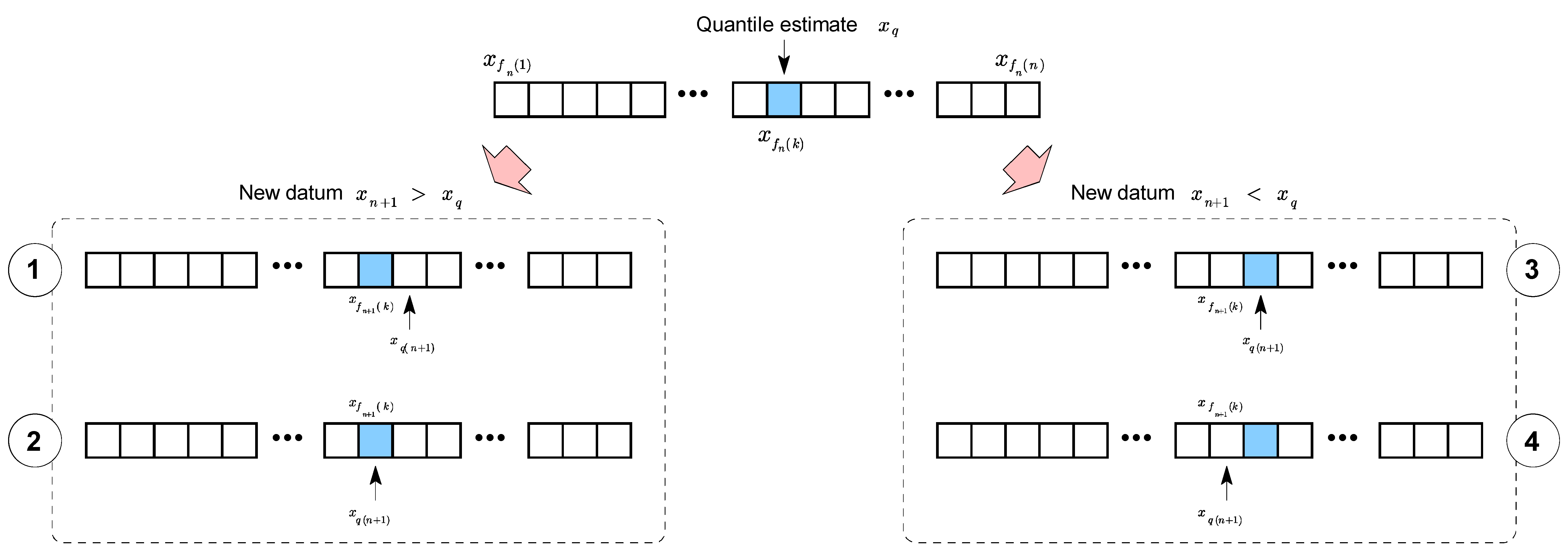
2.4. Targeted Adaptable Sample Algorithm

Having laid out the key theoretical results underpinning our approach, we are now in the position to introduce our quantile estimation algorithm. At the heart of the proposed method is a data structure that comprises two parts. The first of these is an ordered list of data points selected from the input data stream. The second part of the structure is auxiliary information associated with the selected data. Specifically, for each remembered datum, we also maintain an estimate of the number of historical data points whose value is lower than that datum. To understand how the stored information evolves and how it is used to keep track of the current quantile estimate, we now consider the initialization of the structure and the effect that the arrival of a new datum has on it.

2.4.1. Initialization

At the beginning of the operation, i.e., before any stream data have been seen, the buffer is empty. Until the buffer is filled, as each new datum arrives, it is inserted into the correct position in the buffer, which maintains its property of being ordered in a monotonically-increasing manner. At this stage, for every new datum $x_{n+1}$ inserted into the buffer, the exact number of lower value historical data points can be computed and stored in the associated auxiliary structure. If $x_{n+1}$ is inserted into the position k in the buffer and $a_n\left(i\right)$ is the auxiliary value associated with the $i^{\mathrm{th}}$ buffer value after the processing of the first n data points:

$$\begin{array}{c}\hfill a_{n+1}\left(k\right)=\left\{\begin{array}{c}{a}_n\left(k\right)\mathrm{if}{a}_n\left(k\right)\mathrm{exists}\hfill \\ n\mathrm{otherwise}\hfill \end{array}\right.\end{array}$$

(16)

and:

$$\begin{array}{c}\hfill \forall i>k.a_{n+1}\left(i\right)=a_n\left(i\right)+1\end{array}$$

(17)

A value that is already present in the buffer is not inserted as a new buffer entry; rather, the auxiliary counts associated with higher value buffer entries are updated as per Equation (17).

2.4.2. Continuous Operation

The process of initialization can be considered over when the number of unique data points from the input stream exceeds the capacity of the buffer. From this moment on, the insertion of a new datum into the buffer must also involve the removal of an existing datum from the buffer. Our goal is to decide on which new datum should be remembered in the buffer and then which old one should be discarded, in a manner that meets the design aims outlined in Section 2.3.

Let $b_n\left(1\right)<b_n\left(2\right)<\dots <b_n\left(m\right)$ be the values in the buffer after the processing of n data points from the stream, where m is the buffer capacity (size). With the arrival of each new datum $x_{n+1}$, we firstly check if its value is already present in the buffer, i.e., if there exists an index i such that $x_{n+1}=b_n\left(i\right)$. If this is the case, the auxiliary counts corresponding to greater buffer values are simply incremented by one as per Equation (17). If the value $x_{n+1}$ is not present in the buffer, we proceed by finding the index k in the buffer of the current quantile. This is achieved by finding the lowest element $b_k$ in the buffer such that $a_n\left(k\right)/n\ge 1-q$, where q is the target quantile. Then, if the new datum is smaller than the current quantile estimate, i.e., $x_{n+1}<b_k$, and either $k<\lfloor m/2\rfloor$ or $x_{n+1}>b_1$, the new datum $x_{n+1}$ is inserted into the buffer and the largest value in the buffer, $b_m$, discarded. The former case reinforces the central positioning of the current quantile estimate (the current quantile is closer to the high end than the low end of the buffer), while the latter acts so as to decrease the spread of values within the buffer (the value of the lowest element in the buffer is increased, while the highest one is left unchanged). The auxiliary count corresponding to the newly-inserted datum is initialized by linearly interpolating between the counts of buffer values between which the datum is inserted:

$$\begin{array}{c}\hfill a_{n+1}\left(i\right)=a_n\left(i\right)+\frac{x_{n+1}-b_n\left(i\right)}{b_n(j+1)-b_n\left(i\right)}\times \left[a_n(i+1)-a_n\left(i\right)\right],\end{array}$$

(18)

where i is the position in the buffer at which $x_{n+1}$ is inserted. Auxiliary counts corresponding to lower valued buffer elements are left unchanged, while those corresponding to higher valued elements are increased by one:

$$\begin{array}{c}\hfill a_{n+1}\left(j\right)=\left\{\begin{array}{c}{a}_n\left(j\right)\mathrm{for}j<i\hfill \\ a_n\left(j\right)+1\mathrm{for}j>i\hfill \end{array}\right.\end{array}$$

(19)

Similarly, if the new datum is greater than the current quantile estimate, i.e., $x_{n+1}>b_k$, and either $k>\lfloor m/2\rfloor$ or $x_{n+1}<b_m$, the new datum $x_{n+1}$ is inserted into the buffer and the smallest value in the buffer, $b_1$, discarded. All the other steps remain the same.

3. Evaluation and Results

We now turn our attention to the evaluation of the proposed algorithm. In particular, to assess its effectiveness and compare it with the algorithms described in the literature (see Section 1), in this section, we report its performance on two synthetic datasets and three large “real-world” data streams. Our aim is first to use simple synthetic data to study the algorithm in a well-understood and controlled setting, before applying it on corpora collected by systems deployed in practice. Specifically, the ”real-world” streams correspond to motion statistics used by an existing CCTV surveillance system for the detection of abnormalities in video footage. It is important to emphasize that the data we used were not acquired for the purpose of the present work, nor were the cameras installed with the same intention. Rather, we used data that were acquired using existing, operational surveillance systems. In particular, our data came from three CCTV cameras, two of which were located in Mexico and one in Australia. The scenes they overlook are illustrated using a single representative frame per camera in Figure 3.

Table 1. Key statistics of the three real-world datasets used in our evaluation. These were acquired using three existing CCTV cameras in operation in Australia and Mexico.

Data Set	Number of Data Points	Mean Value	Standard Deviation
Stream 1	555,022	$7.81\times {10}^{10}$	$1.65\times {10}^{11}$
Stream 2	10,424,756	$2.25$	$15.92$
Stream 3	1,489,618	$1.51\times {10}^5$	$2.66\times {10}^6$

provides a summary of some of the key statistics of the three datasets. We explain the source of these streams and the nature of the phenomena they represent in further detail in Section 3.1.2.

3.1. Evaluation Data

3.1.1. Synthetic Data

The first synthetic dataset that we used for the evaluation in this paper was a simple stream $x_1,x_2,\dots ,x_{n_1}$ generated by drawing each datum $x_i$ independently from a normal distribution represented by the random variable X:

$$\begin{array}{c}\hfill X\sim \mathcal{N}(5,1)\end{array}$$

(20)

Therefore, this sequence had a stationary distribution. We used $n_1=$ 1,000,000 data points.

The second synthetic dataset was somewhat more complex. Specifically, each datum $y_i$ in the stream $y_1,y_2,\dots ,y_{n_1}$ was generated as follows:

$$\begin{array}{c}\hfill y_i=c_i\times y_i^{\left(1\right)}+(1-c_i)\times y_i^{\left(2\right)}\end{array}$$

(21)

where $c_i$ was drawn from a discrete uniform distribution over the set $\left\{0,1\right\}$ and $y_i^{\left(1\right)}$ and $y_i^{\left(2\right)}$ from normal distributions represented by the random variables $Y_1$ and $Y_2$ respectively:

$$\begin{array}{cc}\hfill Y_1& \sim \mathcal{N}(5,1)\hfill \end{array}$$

(22)

$$\begin{array}{cc}\hfill Y_2& \sim \mathcal{N}(10,4).\hfill \end{array}$$

(23)

In intuitive terms, a datum is generated by flipping a fair coin and then, depending on the outcome, drawing the value either from $Y_1$ or $Y_2$. Notice that this dataset therefore does not have the property of stationarity. As in the first experiment, we used $n_2=$ 1,000,000 data points.

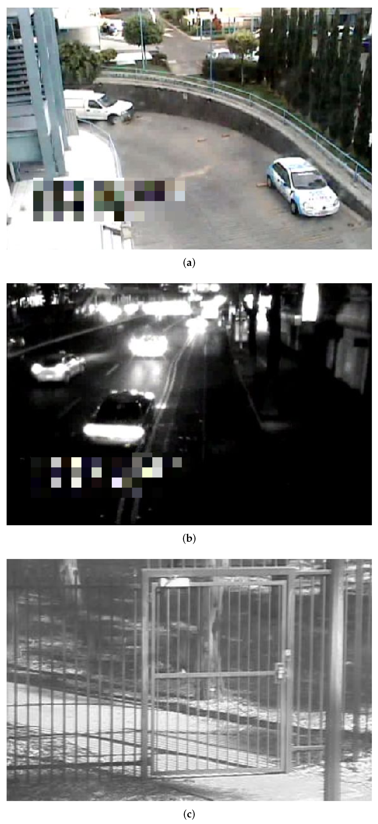
3.1.2. Real-World Surveillance Data

Computer-assisted video surveillance data analysis is of major commercial and law enforcement interest. On a broad scale, systems currently available on the market can be grouped into two categories in terms of their approach. The first group focuses on a relatively small, predefined, and well-understood subset of events or behaviours of interest such as the detection of unattended baggage, violent behaviour, etc. [18,19,20,21,22,23]. The narrow focus of these systems prohibits their applicability in less constrained environments in which a more general capability is required. In addition, these approaches tend to be computationally expensive and error prone, often requiring fine tuning by skilled technicians. This is not practical in many circumstances, for example when hundreds of cameras need to be deployed, as often the case with CCTV systems operated by municipal authorities. The second group of systems approaches the problem of detecting suspicious events at a semantically lower level [24,25]. Their central paradigm is that an unusual behaviour at a high semantic level will be associated with statistically unusual patterns (also “behaviour” in a sense) at a low semantic level: the level of elementary image/video features. Thus, methods of this group detect events of interest by learning the scope of normal variability of low-level patterns and alerting about anything that does not conform to this model of what is expected in a scene, without ”understanding” or interpreting the nature of the event itself. These methods uniformly start with the same procedure for feature extraction. As video data are acquired, firstly a dense optical flow field is computed. Then, to reduce the amount of data that need to be processed, stored, or transmitted, a thresholding operation is performed. This results in a sparse optical flow field whereby only those flow vectors whose magnitude exceeds a certain value are retained; non-maximum suppression is applied here as well. Normal variability within a scene and subsequent novelty detection are achieved using various statistics computed over these data. The three data streams, shown partially in Figure 4, correspond to the values of these statistics (their exact meaning is proprietary and has not been made known fully to the authors of the present paper either; nonetheless, we have obtained permission to make the data public, as we shall do following the acceptance of the paper). Observe the non-stationary nature of the data streams, which is evident both on the long and short time scales (magnifications are shown for additional clarity and insight).

3.2. Results

We now compare the performance of our algorithms with the four alternatives from the literature described in Section 1: (i) the $P^2$ algorithm of Jain and Chlamtac [2], (ii) the random sample-based algorithm of Vitter [15], (iii) the uniform adjustable histogram of Schmeiser and Deutsch [13], and (iv) the data-aligned maximal entropy histogram of Arandjelović et al. [17] (note that in spite of its asymptotically-impressive behaviour, due to the high values of the so-called constant factors “hidden” by asymptotic notation, the algorithm of Munro and Paterson [11] could not be included in the comparison as the total amount of required memory far exceeded that used in our experiments).

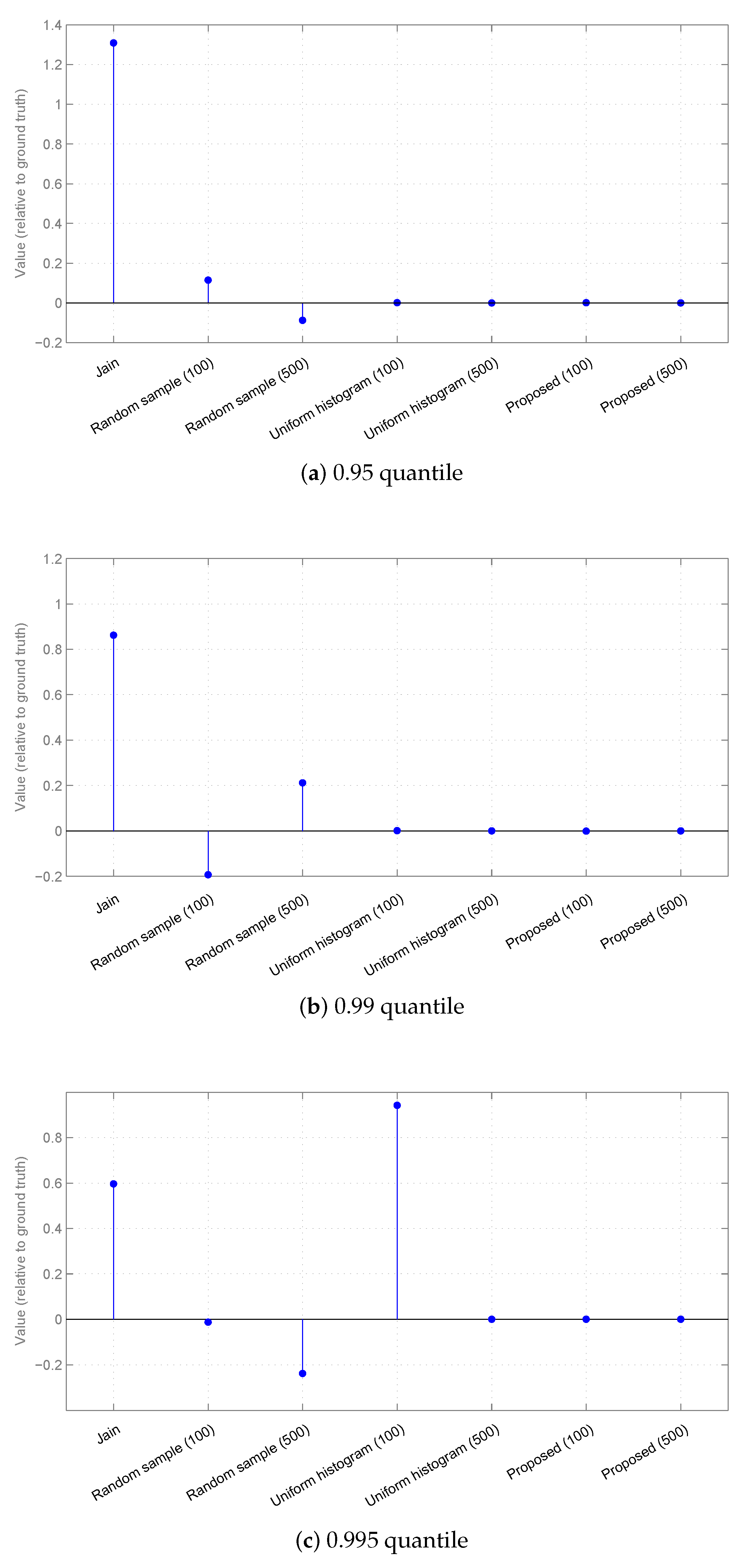
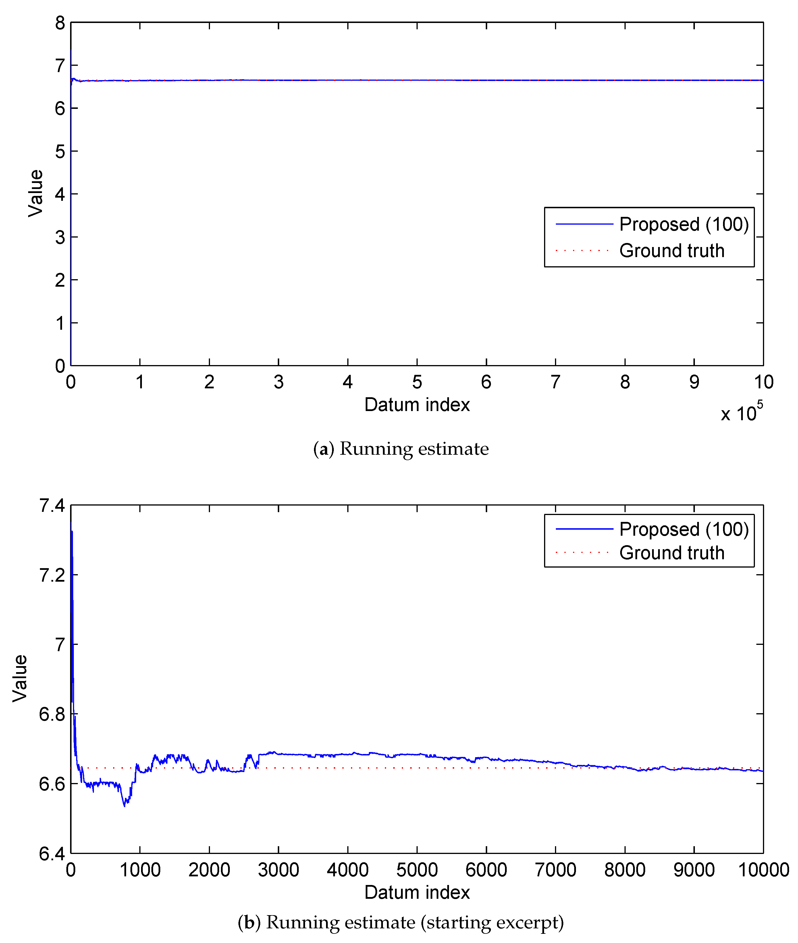
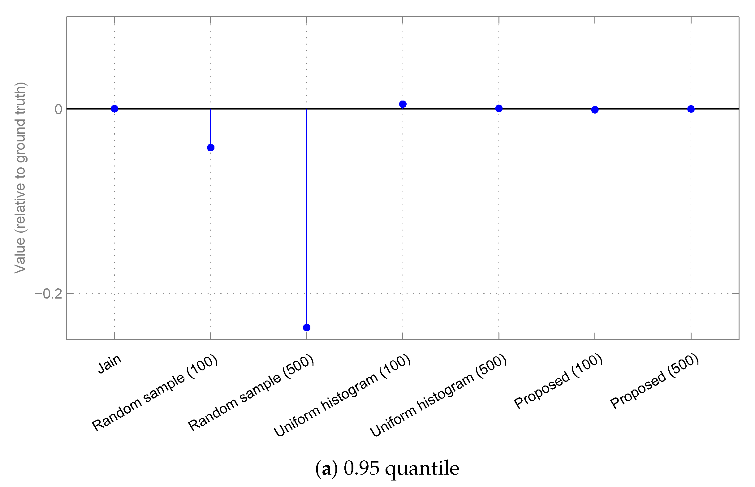
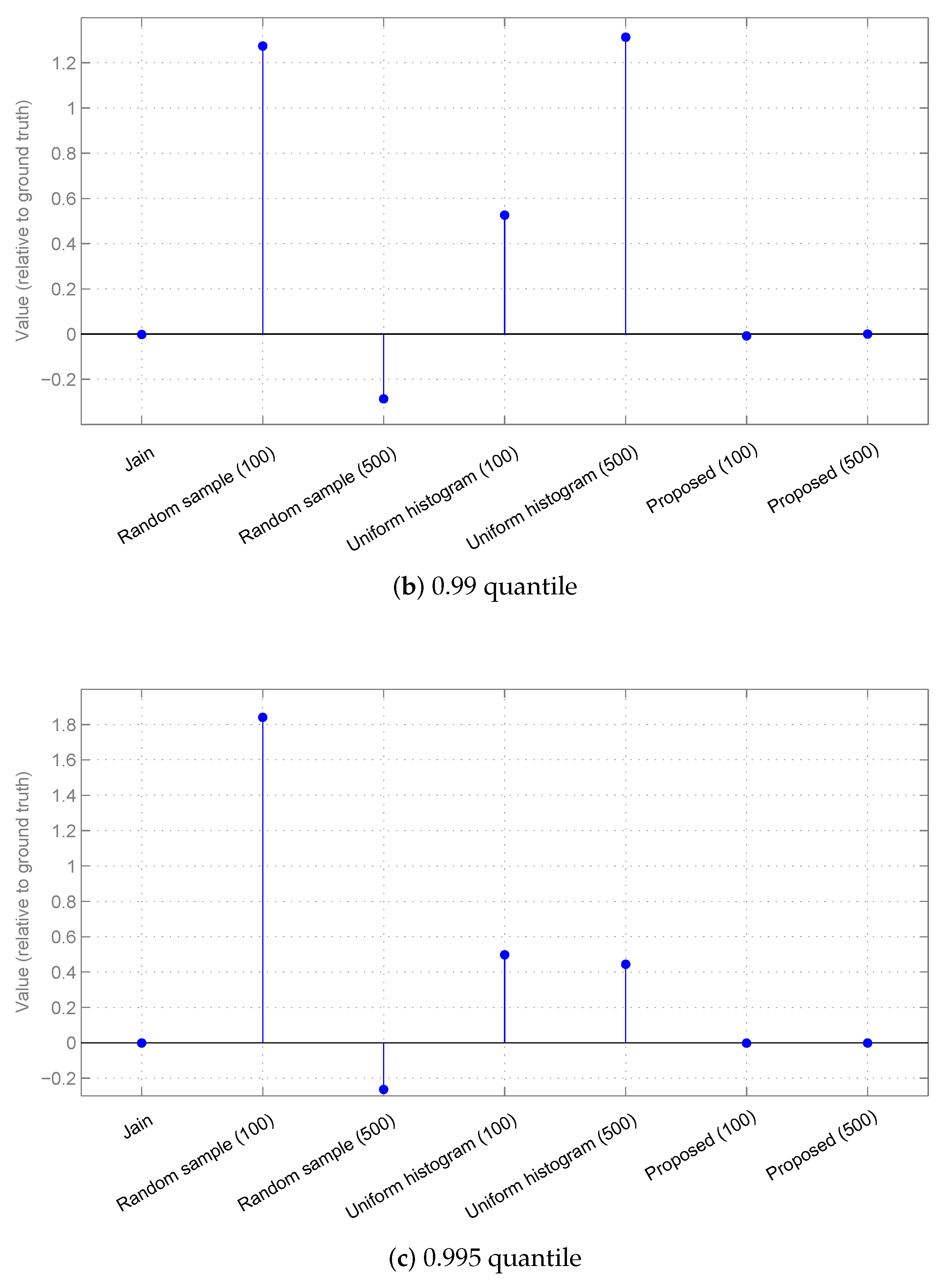
3.2.1. Synthetic Data

We started by examining the results of different algorithms on the first and simplest synthetic stream, with stationary characteristics and data drawn from a normal distribution. Different estimates for the quantile values of 0.95, 0.99, and 0.995 are shown in the stem plots of Figure 5. Several trends are immediately obvious. Firstly, Jain and Chlamtac’s algorithm consistently performed worse, significantly so, than all other methods in all three experiments. This is unsurprising, given that the algorithm uses the least amount of memory. The best performance across all experiments was exhibited by the data-aligned algorithm introduced in this paper, while the relative performances of the sample-based algorithm of Vitter and the uniform histogram method were not immediately clear, one performing better than the other in some cases and vice versa in others. In all experiments, the method proposed in the present paper achieved nearly perfect accuracy, its errors being virtually undetectable with the naked eye at the scale determined by the errors of the remaining methods.

Figure 5 also shows that in all cases except that of the sample-based algorithm of Vitter in the estimation of the 0.995-quantile, a particular method performed better when its available storage space was increased. This observation also is in line with theoretical expectations. However, this is only a partial picture because it offers only a snapshot of the estimates after all data have been processed. The plot in Figure 6 shows the running estimate of the proposed algorithm (blue lines) as progressively more data are seen and reveals further insight. The algorithm converged quickly to the accurate estimate after only a small number of data points from the stream had been processed and showed little fluctuation thereafter.

We now turn our attention to the second synthetic dataset, which, unlike the first one, did not exhibit stationary statistical properties. As before, we first summarize the estimates of three quantile values for different algorithms after all available data were processed. The results are summarized in Figure 7. Most of the conclusions that can be drawn from these mirror those already made on the first synthetic set. The proposed data-aligned bins algorithm consistently performed best and without any deterioration when the buffer size was reduced from 500 to 100. The uniform adjustable histogram of Schmeiser and Deutsch outperformed the sample-based algorithm of Vitter on average, but again exhibited short-lived, but large transient errors.

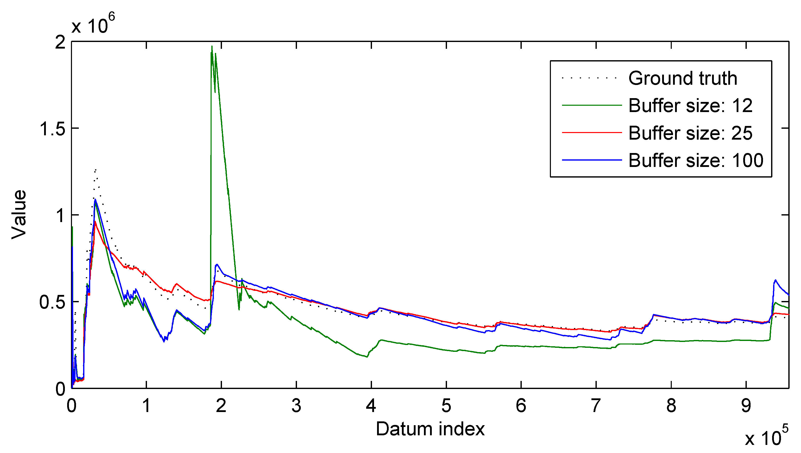
3.2.2. Real-World Surveillance Data

Having gained some understanding of the behaviour of different algorithms in a setting in which input data are well understood and controlled, we applied them to data acquired by a real-world surveillance system. A representative summary of the results is shown in

Table 2. Comparative experimental results.

		Stream 1		Stream 2		Stream 3
Method	Bins	Relative	Absolute	Relative	Absolute	Relative	Absolute
		${\mathit{L}}_1$ Error	${\mathit{L}}_{\mathit{\infty }}$ Error	${\mathit{L}}_1$ Error	${\mathit{L}}_{\mathit{\infty }}$ Error	${\mathit{L}}_1$ Error	${\mathit{L}}_{\mathit{\infty }}$ Error
Targeted adaptable	500	2.1%	1.00 $\times {10}^{11}$	4.7%	24.20	5.2%	4.8 $\times {10}^5$
sample (proposed)	100	1.6%	1.07 $\times {10}^{11}$	9.2%	54.73	3.6%	2.89 $\times {10}^5$
Data-aligned max.	500	1.2%	3.11 $\times {10}^{10}$	0.0%	2.04	0.1%	8.11 $\times {10}^4$
entropy histogram [17]	100	9.6%	2.06 $\times {10}^{11}$	0.0%	1.91	2.6%	3.33 $\times {10}^5$
$P^2$ algorithm [2]	n/a	15.7%	2.77 $\times {10}^{11}$	3.1%	93.04	84.2%	1.55 $\times {10}^6$
Random sample [15]	500	4.6%	1.98 $\times {10}^{11}$	0.7%	38.00	10.4%	5.95 $\times {10}^5$
Equispaced histogram [13]	500	87.1%	1.07 $\times {10}^{12}$	0.1%	80.29	675.1%	4.39 $\times {10}^7$

. It can be readily observed that our method and the method of Arandjelović et al. significantly outperformed other approaches. The $P^2$ and equispaced histogram-based algorithms performed worst, often producing highly inaccurate estimates. For example, on Data Stream 3, which proved to be the most challenging one, the mean relative $L_1$ error of the running quantile estimate of the $P^2$ algorithm was 84.2% and of the equispaced histogram-based method (i.e., the uniform adjustable histogram of Schmeiser and Deutsch) 675.1%. In both cases, such poor performance is to be expected from the underlying theory. The $P^2$ algorithm uses too few salient points and parametric interpolation, which poorly generalizes to streams with arbitrary stochasticity, while the algorithm of Schmeiser and Deutsch experienced a major loss of information every time the histogram boundaries needed to be changed and the histogram stretched to account for a particularly large novel datum. The random sample algorithm of Vitter performed somewhat better, but still substantially worse than the top two methods across all three datasets.

It is interesting to note that in the experiments summarized in Table 2, the data-aligned maximal entropy histogram of Arandjelović et al. outperformed the proposed method. This can be observed consistently across all thee datasets, both in terms of the mean relative $L_1$ error and the absolute $L_{\infty }$ error, and for both buffer capacities (500 and 100 elements). At first, we found this highly surprising given that the data-aligned maximal entropy histogram algorithm approximated the entire distribution of historical data, whereas ours, by design, narrowed its focus to the most relevant part of the distribution. We hypothesized that the reason behind this result lied in the insufficiently challenging input conditions. The first contributing factor was the value of the target quantile and in particular its distance from unity. The experiments in Table 2 used the quantile value of $q=0.95$, which means that both in the case of 500 and 100 element buffers, a significant precision could be reached even with relatively simple binning since $(1-0.95)\times 500=25$ and $(1-0.95)\times 100=5$. Indeed, this is corroborated by the relatively good performance of the random sample algorithm of Vitter discussed previously. In this context, it is also important to observe that in general, some information is lost by interpolation every time a new datum is added to our buffer; recall Equation (18), which was used to initialize the auxiliary count associated with each element in the buffer. While interpolation was also employed by Arandjelović et al., when the target quantile was not close to unity relative to the buffer size, the number of interpolations performed by the simple data-aligned maximal entropy histogram was lower and its underlying model sufficiently flexible to produce an accurate estimate. Consequently, we hypothesized that the advantages of our method would only be fully exhibited for higher quantiles, and we sought to investigate that next.

In the second set of experiments, we compared our method with the data-aligned maximal entropy histogram of Arandjelović et al. using a series of progressively challenging target quantiles. A summary of the results is shown in

Table 3. Comparison of the top two algorithms for high quantiles.

		Proposed Method		Data-Aligned Histogram
Data Set	Quantile	Relative	Absolute	Relative	Absolute	Max Value to Quantile Ratio
		${\mathit{L}}_1$ Error	${\mathit{L}}_{\mathit{\infty }}$ Error	${\mathit{L}}_1$ Error	${\mathit{L}}_{\mathit{\infty }}$ Error
	0.9500	1.6%	1.07 $\times {10}^{11}$	9.6%	2.06 $\times {10}^{11}$	15.8
	0.9900	1.2%	9.59 $\times {10}^{10}$	27.9%	5.69 $\times {10}^{11}$	5.9
Stream 1	0.9950	2.1%	9.27 $\times {10}^{10}$	58.8%	8.48 $\times {10}^{11}$	4.2
	0.9990	0.7%	9.80 $\times {10}^{10}$	48.0%	9.47 $\times {10}^{11}$	2.1
	0.9995	0.3%	2.69 $\times {10}^{10}$	36.8%	8.72 $\times {10}^{11}$	1.5
	0.9500	9.2%	54.73	0.0%	1.91	30.1
	0.9900	2.4%	26.31	0.3%	2.45	2.5
Stream 2	0.9950	0.3%	6.21	0.2%	4.59	1.8
	0.9990	0.2%	16.05	0.4%	30.29	1.4
	0.9995	0.2%	20.17	2.0%	34.44	1.3
	0.9500	3.6%	2.89 $\times {10}^5$	2.6%	3.33 $\times {10}^5$	520.3
	0.9900	1.2%	3.32 $\times {10}^6$	2.4%	3.25 $\times {10}^5$	122.7
Stream 3	0.9950	1.8%	1.40 $\times {10}^6$	480.5%	1.63 $\times {10}^8$	60.9
	0.9990	1.6%	3.35 $\times {10}^6$	368.6%	2.35 $\times {10}^7$	11.7
	0.9995	4.2%	1.30 $\times {10}^7$	364.2%	2.34 $\times {10}^8$	7.2

. It is readily apparent that this set of results fully supported our hypothesis. While our algorithm showed an improvement in performance as the value of the target quantile was increased, the opposite was true for the data-aligned maximal entropy histogram, which performed progressively worse. Dataset 3 again proved to be the most challenging one: the data-aligned maximal entropy histogram producing grossly inaccurate estimates for quantile values of over $0.99$. For example, on Stream 3 for the target quantile of $0.999$, the data-aligned maximal entropy histogram achieved an average relative $L_1$ error of 368.6%, while the proposed algorithm showed remarkable accuracy and an error of 1.6%. The same observations can be made by considering the absolute $L_{\infty }$ error, i.e., the greatest error in the running quantile estimates, which were respectively 2.35 $\times {10}^7$ and 3.35 $\times {10}^6$, a difference of approximately an order of magnitude.

Table 3 also includes a column (right-most) showing the ratio of the maximal stream value and the ground truth for the target quantile. We sought to examine if a particularly high ratio predicts poor performance of the data-aligned maximal entropy histogram, which may be expected given that throughout its operation, the algorithm approximates the entire distribution of historical data. We found this not to be the case, which can be explained by the allocation of bin ranges according to the maximum entropy principle and the alignment of the bin boundaries with data; please see the original publication for a detailed description of the method [17].

Lastly, we sought to analyse the performance of the proposed method in additional detail. Figure 8 shows on an example of the running ground truth of the target quantile ($q=0.95$) and the estimates of our algorithm for different bin sizes on the most challenging Data Stream 3. It is remarkable to observe that our method consistently achieved a highly accurate estimate even when the available buffer capacity was severely restricted (to 12 bins). In Figure 9, the same example run was used to illustrate the success of our algorithm in achieving one of the key ideas behind the method, that of adapting the data sample retained in the buffer so as to maintain the position of the current quantile estimate in the buffer as close to its centre as possible (see Section 2.3). As the plot clearly shows, both in the case of a buffer with the capacity of 100 and 12 (the results for only two buffer sizes are shown to reduce clutter), the central positioning of the quantile estimate was maintained very tightly throughout the processing of the stream. Similarly, the success of our algorithm in achieving tight sampling of the data distribution around the target quantile is illustrated in the plot in Figure 10. This plot shows that unlike the random sample-based algorithm of Vitter [15] or the uniform adjustable histogram of Schmeiser and Deutsch [13], which retained a sample from a wide range of values, our method utilized the available memory efficiently by focusing on a narrow spread of values around the current quantile estimate. Note that the spread of values in the buffer experienced intermittent and transient increases when there was a burst of high-valued data points in preparation for a potentially large quantile change, but thereafter quickly adapted to the correct part of the distribution. The variation in the mean buffer spread with the buffer size and target quantile is shown in Figure 11. Lastly, the variation in the accuracy of our algorithm’s estimate with the buffer size is analysed in Figure 12. Unlike any of the existing algorithms, our method exhibited very gradual and graceful degradation in performance and still achieved remarkable accuracy even with a severely restricted buffer capacity.

4. Summary and Conclusions

In this paper, we addressed the problem of estimating a desired quantile of a dataset. Our goal was specifically to perform quantile estimation on a data stream when the available working memory was limited (constant), prohibiting the storage of all historical data. This problem is ubiquitous in computer vision and signal processing and has been addressed by a number of researchers in the past. We show that a major shortcoming of the existing methods lies in their usually implicit assumption that the data are being generated by a stationary process. This assumption was invalidated in most practical applications, as we illustrated using real-world data extracted from surveillance videos.

Therefore, we introduced a novel algorithm that deals with the described challenges effectively. The algorithm was founded on an important theoretical result, which we derived and which showed that the change in the quantile of a stream was constrained regardless of the stochastic properties of the data. This result led us to a set of high-level design goals for an effective estimation methodology and a novel algorithm that implemented the aforementioned design goals. This was achieved by retaining a sample of data values in a manner that adapted to the changes in the distribution of data and progressively narrowed down its focus in the periods of quasi-stationary stochasticity.

The proposed algorithm was evaluated and compared against the existing alternatives described in the literature using three large data streams. These data were extracted from CCTV footage, not collected specifically for the purposes of this work, and represent specific motion characteristics over time, which were used by semi-automatic surveillance analytics systems to alert about abnormalities in a scene. Our evaluation conclusively demonstrated a vastly superior performance of our algorithm. The highly non-stationary nature of the evaluation data was shown to cause major problems for the existing algorithms, often leading to grossly inaccurate quantile estimates; in contrast, our method was virtually unaffected by this. What is more, our experiments demonstrated that the superior performance of our algorithm could be maintained effectively while drastically reducing the working memory size in comparison with the methods from the literature.

References

1. Beykikhoshk, A.; Arandjelović, O.; Phung, D.; Venkatesh, S.; Caelli, T. Data-mining Twitter and the autism spectrum disorder: A pilot study. In Proceedings of the IEEE/ACM International Conference on Advances in Social Network Analysis and Mining, Beijing, China, 17–20 August 2014; IEEE: Piscataway, NJ, USA, 2014; pp. 349–356. [Google Scholar]
2. Jain, R.; Chlamtac, I. The P2 Algorithm for Dynamic Calculation of Quantiles and Histograms Without Storing Observations. Commun. ACM 1985, 28, 1076–1085. [Google Scholar] [CrossRef]
3. Adler, R.; Feldman, R.; Taqqu, M. (Eds.) A Practical Guide to Heavy Tails; Statistical Techniques and Applications, Birkhäuser: Basel, Switzerland, 1998. [Google Scholar]
4. Sgouropoulos, N.; Yao, Q.; Yastremiz, C. Matching Quantiles Estimation; Technical Report; London School of Economics: London, UK, 2013. [Google Scholar]
5. Macindoe, A.; Arandjelović, O. A standardized, and extensible framework for comparative analysis of quantitative finance algorithms—An open-source solution, and examples of baseline experiments with discussion. In Proceedings of the IEEE International Conference on Big Knowledge, Singapore, 17–18 November 2018; IEEE: Piscataway, NJ, USA, 2018; pp. 409–414. [Google Scholar]
6. Buragohain, C.; Suri, S. Encyclopedia of Database Systems; Chapter Quantiles on Streams; Springer: New York, NY, USA, 2009; pp. 2235–2240. [Google Scholar]
7. Cormode, G.; Johnson, T.; Korn, F.; Muthukrishnany, S.; Spatscheck, O.; Srivastava, D. Holistic UDAFs at Streaming Speeds. In Proceedings of the ACM SIGMOD International Conference on Management of Data, Paris, France, 13–18 June 2004; ACM: New York, NY, USA, 2004; pp. 35–46. [Google Scholar]
8. Pham, D.; Arandjelović, O.; Venkatesh, S. Detection of dynamic background due to swaying movements from motion features. IEEE Trans. Image Process. 2015, 24, 332–344. [Google Scholar] [CrossRef] [PubMed]
9. Arandjelović, O.; Pham, D.; Venkatesh, S. The adaptable buffer algorithm for high quantile estimation in non-stationary data streams. In Proceedings of the IEEE International Joint Conference on Neural Networks, Washington, DC, USA, 10–16 July 2015; IEEE: Piscataway, NJ, USA, 2015; pp. 1–7. [Google Scholar]
10. Guha, S.; McGregor, A. Stream Order and Order Statistics: Quantile Estimation in Random-Order Streams. SIAM J. Comput. 2009, 38, 2044–2059. [Google Scholar] [CrossRef] [Green Version]
11. Munro, J.I.; Paterson, M. Selection and sorting with limited storage. Theor. Comput. Sci. 1980, 12, 315–323. [Google Scholar] [CrossRef] [Green Version]
12. Gurajada, A.P.; Srivastava, J. Equidepth Partitioning of a Data Set Based on Finding its Medians; Technical Report TR 90-24; Computer Science Department, University of Minnesota: Minneapolis, MN, USA, 1990. [Google Scholar]
13. Schmeiser, B.W.; Deutsch, S.J. Quantile Estimation from Grouped Data: The Cell Midpoint. Commun. Stat. Simul. Comput. 1977, B6, 221–234. [Google Scholar] [CrossRef]
14. McDermott, J.P.; Babu, G.J.; Liechty, J.C.; Lin, D.K.J. Data skeletons: Simultaneous estimation of multiple quantiles for massive streaming datasets with applications to density estimation. Bayesian Anal. 2007, 17, 311–321. [Google Scholar] [CrossRef]
15. Vitter, J.S. Random sampling with a reservoir. ACM Trans. Math. Softw. 1985, 11, 37–57. [Google Scholar] [CrossRef] [Green Version]
16. Cormode, G.; Muthukrishnany, S. An improved data stream summary: The count-min sketch and its applications. J. Algorithms 2005, 55, 58–75. [Google Scholar] [CrossRef]
17. Arandjelović, O.; Pham, D.; Venkatesh, S. Stream quantiles via maximal entropy histograms. In Proceedings of the International Conference on Neural Information Processing, Kuching, Malaysia, 3–6 November 2014; Springer: Cham, Switzerland, 2014; Volume II, pp. 327–334. [Google Scholar]
18. Philips Electronics, N.V. A Surveillance System with Suspicious Behaviour Detection. U.S. Patent Application No. 10/014,228, 11 December 2001. [Google Scholar]
19. Lavee, G.; Khan, L.; Thuraisingham, B. A framework for a video analysis tool for suspicious event detection. Multimed. Tools Appl. 2007, 35, 109–123. [Google Scholar] [CrossRef]
20. Zhou, H.; Zhang, J.; Wang, L.; Zhang, Z.; Brown, L.M. Sparse representation for event recognition in video surveillance. Pattern Recognit. 2013, 46, 1748–1749. [Google Scholar] [CrossRef]
21. Bregonzio, M.; Xiang, T.; Gong, S. Fusing appearance and distribution information of interest points for action recognition. Pattern Recognit. 2012, 45, 1220–1234. [Google Scholar] [CrossRef]
22. Tran, K.N.; Kakadiaris, I.A.; Shah, S.K. Part-based motion descriptor image for human action recognition. Pattern Recognit. 2012, 45, 2562–2572. [Google Scholar] [CrossRef]
23. Wang, H.; Yuan, C.; Hu, W.; Sun, C. Supervised class-specific dictionary learning for sparse modeling in action recognition. Pattern Recognit. 2012, 45, 3902–3911. [Google Scholar] [CrossRef]
24. Intellvisions. iQ-Prisons. Available online: http://www.intellvisions.com/ (accessed on 23 July 2019).
25. iCetana. Available online: https://icetana.com (accessed on 23 July 2019).
Figure 1. An example of a rapid change in the value of a quantile (specifically, the 0.95-quantile in this case) on a real-world data stream.
Make 01 00049 g001
Figure 2. An illustration of the derived result that constrains the changes in the target quantile with the arrival of a single new datum. At the top of the diagram is the ordered list of historical stream values x f n ( 1 ) < x f n ( 2 ) < < x f n ( n ) . The value corresponding to the current quantile estimate x q ( n ) (shown as being pointed to by an arrow) is highlighted in light blue. Following the arrival of the new datum x n + 1 , there are four different possible outcomes (labelled as 14).
Make 01 00049 g002
Figure 3. (a–c) Screenshots of the three scenes used to acquire the data used in our experiments. Note that these are real, operational CCTV cameras, which were not specifically installed for the purpose of data acquisition for the present work. See Figure 4 as well.
Make 01 00049 g003
Figure 4. The three large data streams used to evaluate the performance of the proposed algorithms and to compare with the approaches previously described in the literature. See Figure 3 as well.
Make 01 00049 g004
Figure 5. A comparison of different methods on the first synthetic datasets used in this paper. This stream has stationary statistical characteristics and was generated by drawing each datum (of 1,000,000 in total) independently from the normal distribution N (5, 1). The label “Jain” refers to the P2 algorithm of Jain and Chlamtac [2], “Sample” to the random sample-based algorithm of Vitter [15], “Uniform” to the uniform adjustable histogram of Schmeiser and Deutsch [13], and “Proposed” to our method described in Section 2.4. The number in brackets after a method name signifies the size of its buffer i.e., available working memory.
Make 01 00049 g005
Figure 6. Running estimate of the 0.95-quantile produced by the proposed algorithm on our first synthetic dataset.
Make 01 00049 g006
Figure 7. A comparison of different methods on the second synthetic dataset used in this paper. Each datum of this stream (of 1,000,000 in total) was generated by flipping a fair coin and then, depending on the outcome, drawing the value either from the normal distribution N (5, 1) or from N (10, 4). Notice that the data are not stationary in nature. The number in brackets after a method name signifies the size of its buffer, i.e., available working memory.
Make 01 00049 g007aMake 01 00049 g007b
Figure 8. An example running ground truth of the target quantile ( q = 0 . 95 ) and the estimates of our algorithm for different bin sizes on Data Stream 3. It is remarkable to observe that our method achieved a consistently highly accurate estimate even when the available buffer capacity was severely restricted (down to only 12 bins).
Make 01 00049 g008
Figure 9. Our algorithm is highly successful at achieving one of the key ideas behind the method, that of adapting the data sample retained in the buffer so as to maintain the position of the current quantile estimate in the buffer as close to its centre as possible (see Section 2.3). Both in the case of a buffer with a capacity of 100 and 12 (the results for only two buffer sizes are shown to reduce clutter), the central positioning of the quantile estimate is maintained very tightly throughout the processing of the stream.
Make 01 00049 g009
Figure 10. The success of our algorithm in achieving tight sampling of the data distribution around the target quantile. Unlike the random sample based algorithm of Vitter [15] or the uniform adjustable histogram of Schmeiser and Deutsch [13], which retain a sample from a wide range of values, our method utilizes the available memory efficiently by focusing on a narrow spread of values around the current quantile estimate. While the spread of values in the buffer experiences intermittent and transient increases when there is a burst of high-valued data points in preparation for a potentially large quantile change, thereafter it quickly adapts to the correct part of the distribution.
Make 01 00049 g010
Figure 11. The variation in the mean buffer spread with the buffer size and target quantile on Data Stream 3.
Make 01 00049 g011
Figure 12. The variation in the accuracy of our algorithm’s estimate with the buffer size on Data Stream 3. Unlike any of the existing algorithms, our method exhibits very gradual and graceful degradation in performance and still achieves remarkable accuracy even with a severely restricted buffer capacity.
Make 01 00049 g012