Article

Pattern Classification by the Hotelling Statistic and Application to Knee Osteoarthritis Kinematic Signals

1
INRS-Énergie matériaux et télécommunications, Montreal, QC H5A 1K6, Canada
2
Centre de recherche LICEF, TELUQ university, Montreal, QC H2S 3L5, Canada
3
Laboratoire de recherche en imagerie et orthopédie, Centre de recherche du CHUM, Montreal, QC H2X 0A9, Canada
*
Author to whom correspondence should be addressed.
Mach. Learn. Knowl. Extr. 2019, 1(3), 768-784; https://doi.org/10.3390/make1030045
Submission received: 22 March 2019 / Revised: 25 June 2019 / Accepted: 26 June 2019 / Published: 5 July 2019
(This article belongs to the Section Learning)

Abstract

:
The analysis of knee kinematic data, which come in the form of a small sample of discrete curves that describe repeated measurements of the temporal variation of each of the knee three fundamental angles of rotation during a subject walking cycle, can inform knee pathology classification because, in general, different pathologies have different kinematic data patterns. However, high data dimensionality and the scarcity of reference data, which characterize this type of application, challenge classification and make it prone to error, a problem Duda and Hart refer to as the curse of dimensionality. The purpose of this study is to investigate a sample-based classifier which evaluates data proximity by the two-sample Hotelling T 2 statistic. This classifier uses the whole sample of an individual’s measurements for a better support to classification, and the Hotelling T 2 hypothesis testing made applicable by dimensionality reduction. This method was able to discriminate between femero-rotulian (FR) and femero-tibial (FT) knee osteoarthritis kinematic data with an accuracy of 88.1 % , outperforming significantly current state-of-the-art methods which addressed similar problems. Extended to the much harder three-class problem involving pathology categories FR and FT, as well as category FR-FT which represents the incidence of both diseases FR and FT in a same individual, the scheme was able to reach a performance that justifies its further use and investigation in this and other similar applications.

1. Introduction

High-dimensional data classification can be quite problematic when the supporting sample is small: this is what Duda and Hart [1] call the curse of dimensionality, a condition known to degrade the performance of otherwise potent classifiers [2]. The problem occurs in several subjects, microarray analysis, for instance, where there are tens of thousands of characteristic genes to analyze but only hundreds of observations, and biomedical engineering data analysis where there can be hundreds of classification characteristic variables but samples of only tens of observations.
Investigations of small size dataset classification run along two basic veins. Along one vein, conventional pattern recognition schemes are adapted to conform to specificities of small datasets. Prominent methods, emphasized in face recognition, use linear discriminant analysis (LDA) algorithms [3,4,5,6]. Although LDA has been useful in applications such as face recognition, it does not necessarily generalize to data of other applications, particularly time series signals, the type of data we investigate in this study. Along the second vein of investigation, artificial data are synthesized, when possible, that follow the shape of reference real data and subsequently used with more general classifiers that require large amounts of data, such as neural networks. However, data synthesis, which had some application in medical imaging [7,8], may not be applicable or feasible, as with knee kinematic time series data which we investigate in this study.
Knee kinematic data are in the form of discrete curves, recorded as high-dimensional vectors that describe the temporal variation of each of the three fundamental angles of knee rotation during a walking cycle, namely the abduction/adduction angle, with respect to the frontal plane, the flexion/extension angle, with respect to the sagittal plane, and internal/external angle, with respect to the transverse plane. For any given subject, the measurements are repeated several times to yield a small sample of discrete curves. A measurement curve is generally preprocessed to remove unwanted distortions, and re-sampled to about 100 equally spaced points [9,10], in which case the data dimension is about 300 (Figure 2). The size of a measurement sample is typically 10 to 15.
Knee kinematic data classification can inform diagnosis [11] and, therefore, assist therapy [12], of knee musculoskeletal pathologies, such as those of the osteoarthritis category (OA) [13,14,15,16,17,18]. Current classifiers commonly average the kinematic curves of a subject’s sample of measurements and then use the resulting average to describe the subject’s knee movement for the purpose of subsequent classification. However, averaging may suppress relevant information in the data. Therefore, instead of collapsing a subject’s sample of measurements to its average, or other single representative curve [13,14,15], it would be more expedient to retain all the curves for a more informative support to classification. The classifier we propose exploits this rather manifest but nevertheless important fact that current studies have generally overlooked. This classifier assigns class membership to observations of knee kinematic data using the Hotelling T 2 test [19,20] on a reduced-dimensionality representation of the data. The Hotelling T 2 statistic is a multivariate generalization of the univariate Student t statistic. The hypothesis test in this study evaluates kinematic data sample similarity for classification to use. Therefore, classification proceeds as usual: an observation is assigned to the most likely category, except that the observation here is a sample of feature vectors rather than a single such vector, and that similarity in feature space, which enters class membership decision, is evaluated using the two-sample Hotelling T 2 statistic rather than a distance function or other form of vector proximity. This will be described in greater detail subsequently.
Beyond its basic use in a sample-based generalization of the nearest neighbor classifier, as proposed in this study, the Hotelling statistic can potentially serve to evaluate similarity in general similarity-based pattern classification, whenever the measurement data come as samples of vectors rather than single vectors as it is usually the case. Similarity-based methods include nearest neighbors classification, pattern clustering, artificial intelligence instance-based and case-based reasoning, and neural network memory representation [21]. Along the vein of neural network memory representation, for instance, we investigated a sample-based generalization of the Kohonen associative memory [22]. The main purpose of a Kohonen memory is to offer a means for a richer, more informative description of classes by unsupervised mapping of the data onto a network of spatially organized feature nodes that reflect the spread of the application data. Basically, the sample-based generalization in [22] replaces the Euclidean distance of the original Kohonen neural network by a Hotelling statistic similarity, so as to accommodate inputs that are samples of vector data.
The remainder of this paper is organized as follows: Section 2 describes the two-sample Hotelling T 2 test and classification. Section 3 describes the dimensionality reduction and Section 4 details the experimental results. Finally, Section 5 presents conclusions.

2. The Two-Sample Hotelling T 2 Test and Classification

Let X = { x 1 , , x n } and Y = { y 1 , , y m } be two samples, of size n and m, of independent realizations of two d-variate multinomial variables of equal covariance matrices and with means μ x and μ y .
Let x ¯ and y ¯ be the sample means of S X and S Y , respectively:
x ¯ = 1 n i = 1 n x i ; y ¯ = 1 m i = 1 m y i
and C x , C y the sample covariances:
C x = 1 n 1 i = 1 n ( x i x ¯ ) ( x i x ¯ ) T , C y = 1 m 1 i = 1 m ( y i y ¯ ) ( y i y ¯ ) T .
The two-sample Hotelling statistic is then given by [19]:
T 2 = n m n + m ( x ¯ y ¯ ) T C 1 ( x ¯ y ¯ ) ,
where C is the pooled covariance estimate of x ¯ y ¯ given by:
C = ( n 1 ) C x + ( m 1 ) C y n + m 2 .
For large samples, the distribution of T 2 under the null hypothesis H 0 : μ x = μ y against the hypothesis H 1 : μ x μ y ([20]) is approximately χ 2 (chi-squared) with d degrees of freedom, and for small sample sizes, as in our case, it is better approximated by the F distribution with d degrees of freedom for the numerator, and n + m 1 d for the denominator, which, therefore, takes into account the size of the samples, m and n, and the dimension d of the data [20]:
n + m d 1 ( n + m 2 ) d T 2 F ( d , n + m 1 d ) .
The F distribution in Equation (5) can be a good approximation of the T 2 statistic distribution when the dimension of the data are less than the size of the samples [20]. Dimensionality reduction provides, as in this study, a means to satisfy this condition. This will be taken up in Section 3.
In statistical hypothesis testing, the p-value serves to test the statistical significance of the null hypothesis H 0 . The test functions about a reductio ad absurdum argument, according to which rejection of hypothesis H 0 validates the (single) alternate hypothesis H 1 , its logical complement. Therefore, classification can proceed in the following manner. For l = 1 , , c , let { R j l } j be the reference set of samples of class l, and let X be a sample to classify. Let s j l be the observed T 2 statistic for X and a reference sample R j l and p j l the corresponding the p-value. Using the right tail event, i.e., the right tail of the approximating F distribution, the p-value is:
p j l = 1 0 s j l F d s .
The smaller this p-value, the higher the statistical significance of the observed statistic, and if less than an arbitrarily set small threshold, called critical value, H 0 can be rejected, implying, according to the reductio ad absurdum argument that H 1 can be accepted. In a context of classification, accepting H 0 can be interpreted to mean that the two observed samples, X and R j l , are of the same class, and accepting the alternate H 1 instead that they are not. Considering also that the T 2 statistic is (positively) proportional to the Mahalanobis distance between the samples [20,23], classification can use the following decision rule: Assign X to class l 0 corresponding to the largest p-value:
l 0 = arg max l { max j p j l } .
However, since the p-value is a monotonically decreasing function of the statistic, it is sufficient to use the rule that assigns the observed sample X to the class that yields the T 2 statistic of lowest value, foregoing—thus the need to actually compute p-values. One can easily see that classification by the Hotelling test as presented here is a generalization of the nearest neighbor classifier where pattern similarity is between two samples of characteristic vectors, rather than between two single such vectors. The scheme can be condensed as the following pseudo-code (Algorithm 1):
Algorithm 1: Hotelling T 2 hypothesis testing and classification
Make 01 00045 i001

3. Dimensionality Reduction

For a hypothesis test for a small-sample statistic such as Hotelling T 2 to be applicable, the dimension of the data must be less than the size of the samples in the test [20]. Therefore, we precede classification by dimensionality reduction to satisfy this requirement. We performed a Daubechies wavelet transform [24], often used for dimensionality reduction in pattern analysis and classification [25]. The relevant wavelet coefficients of the transform are then selected using a filter-based feature selection method.

3.1. Wavelet Representation

A wavelet method of representation retains of the data wavelet decomposition coefficients only those which correspond to a predetermined energy of the transformed signal [26,27,28]. A significant advantage of the wavelet representation is that a decomposition depends on the data item to describe, not on other data, in contrast to other common feature selection methods such as principal component analysis (PCA) or singular value decomposition (SVD).

3.2. Filter-Based Feature Selection

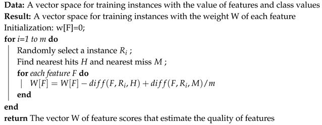
Feature selection identifies the discriminant features in a given set of original features. In our case, features are wavelet coefficients. In general, feature selection reduces the complexity of describing and implementing an expert system, increasing its efficiency thereof. The selection of the best features to use in computer-aided diagnostic systems is a key issue in obtaining a satisfactory performance [2]. We investigated a filter-based feature selection method that consists of determining the subset of features with the highest predictive power. More specifically, we used the ReliefF algorithm, which is one of the most successful filtering feature selection scheme [29]. The scheme is summarized from a top-level point of view by Algorithm 2 below.
Basically, the ReliefF algorithm weighs the importance of each feature according to its relevance to the class. Initially, all weights W [ F ] are set to zero and then updated iteratively. At each iteration, the ReliefF selects randomly an instance R i and searches for its k nearest neighbors of the same class, called nearest hits H, and also k-nearest neighbors from each of the different classes, called nearest misses M. The quality estimation of the all the features is then updated depending on their values R i , hits H and misses M as described in the following pseudo-code.
For two instances I 1 and I 2 , d i f f ( A , I 1 , I 2 ) calculates differences between the class of the feature F:
d i f f ( F , I 1 , I 2 ) = 0 , if v a l u e s ( F , I 1 ) = v a l u e s ( F , I 2 ) , 1 , if v a l u e s ( F , I 1 ) v a l u e s ( F , I 2 ) .
The output of the ReliefF algorithm is a weight for each feature, where higher weights indicate better predictive features, so that a ranking of the features is obtained. In our application, this results in the selection of wavelet coefficient that best discriminate the knee pathologies in study.
Algorithm 2: ReliefF Algorithm
Make 01 00045 i002

4. Experimental Results

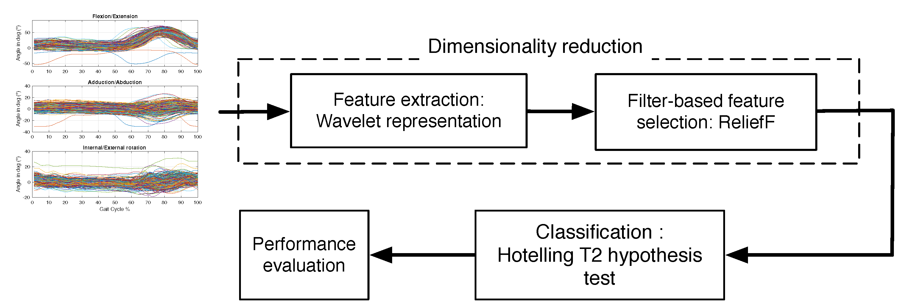
The functional diagram of the knee kinematic data classification method proposed in this study is illustrated in Figure 1. Following data collection and preprocessing, the study proceeds in three main steps: dimensionality reduction, which includes features extraction and selection, classification of the kinematic data of reduced dimension using the Hotteling T 2 and, finally, performance evaluation.
Experiments have been performed using osteoarthritis knee kinematic data, namely flexion/extension, abduction/adduction, and internal/External rotation angles. For each participant, the kinematic curves are recorded several times, typically 12 to 15 times, giving a sample of independent realizations per participant. We conducted two validation experiments using the osteoarthritis data described in Section 4.1. The first experiment considered two classes, C 1 and C 2 . Class C 1 represents patients with femoro-tibial osteoarthritis knee osteoarthritis (FT) and C 2 represents patients with femoro-rotular knee osteoarthritis (FR). The dataset used in this first experiment (DS1) was obtained from 42 patients, 21 in each class. The purpose of the second experiment is to show the complexity brought in by the inclusion of an additional class of data from patients with both FR and FT diseases (class C 3 ) forming the data set DS2 of 63 participants.
Using the leave-one-out cross validation procedure, the classifiers performance was evaluated in terms of the accuracy (Acc) over all test data, i.e., data from all test data classes, as well as classification accuracy per class. Given a dataset of cardinality N, the leave-one-out testing method is a standard procedure to evaluate a classifier potency that consists of using in turn each dataset element for tests while the remaining N 1 elements serve to train the classifier. The classification rate is then taken to be the average of the N one-sample classification results. Performance is presented in the form of a confusion matrix where each row represents the instances in a predicted class and each column represents the instances in an actual class (ground truth).

4.1. Knee Kinematic Data Collection

The data collection was approved by institutional ethics committees of the University of Montreal Hospital Research Center (Reference numbers CE 10.001-BSP and BD 07.001-BSP) and of the École de technologie supérieure (Reference numbers H20100301 and H20170901). All subjects provided written informed consent before the studies began. The participants data are of the confidential category and cannot be put in an open repository for unrestricted public access. However, they could be made available upon request provided a statement of confidentiality is signed.
The kinematic data collection was performed using a noninvasive knee marker attachment apparatus, the KneeKG system [30]. The system is placed on the participant’s knee to record the three-dimensional (3D) knee kinematics during two trials of 25 s. The device is first calibrated with respect to the reference points and axes which serve to measure the knee kinematics signals with respect to the frontal, sagittal, and transverse planes from each participant while walking on a conventional treadmill at a self-selected comfortable speed. Accuracy of the attachment system was assessed in studies which evaluated the mean repeatability of measures ranging from 0.4 degree to 0.8 degree for knee rotation angles and from 0.8 to 2.2 mm for translation [31]. Intra- and inter-observer reliability of the attachment system for recording 3D knee kinematics during gait was also ascertained [32]. The measurements give three kinematic curves, one for each angle. Curves are normalized by resampling to some number of equally spaced points [31], one hundred in this study, corresponding to the gait cycle percentage (as illustrated in Figure 2, 1 % corresponds to the initial contact and 100 % to the end of the swing phase).
Because a participant’s gait is not identical from one cycle to another, the kinematic curves are recorded several times, for any given participant, typically ten to fifteen times, and then averaged under the informal assumption that undesirable outlying measurements are present and the effect of which on classification must be inhibited. As a result, current methods have invariably taken the average curves to be the participant’s representative curve in subsequent analysis and classification of knee movement data. In this study, as we mentioned earlier, all of the recorded curves are retained and used together as a sample, rather than collapsing them into a single curve of representation (Figure 2) because such a collapse more often than not suppresses information that might be relevant to the identification of the underlying data class.
The data in this study come from patients with knee osteoarthritis (OA). The diseases considered are femerotibial knee osteoarthritis (FT), femero-rotulian knee osteoarthritis (FR), and occurrence of both FT and FR (designated FT-FR). Patients with symptomatic OA of the knee were recruited from the hospital community. They were diagnosed by a physiatrist, according to the American College of Rheumatology (ACR) criteria (Arden 2006), and with radiographic evidence of OA. Patients were excluded if they had a vestibular or neurological condition, musculoskeletal disorders other than knee OA, a history of lower extremity injury, and any condition affecting their ability to walk on a treadmill, or if they had already participated in a physiotherapy program.
The dataset contains measurements from 21 patients from each class. The demographic characteristics of the data in the three classes are shown in Table 1.

4.2. Feature Extraction and Selection

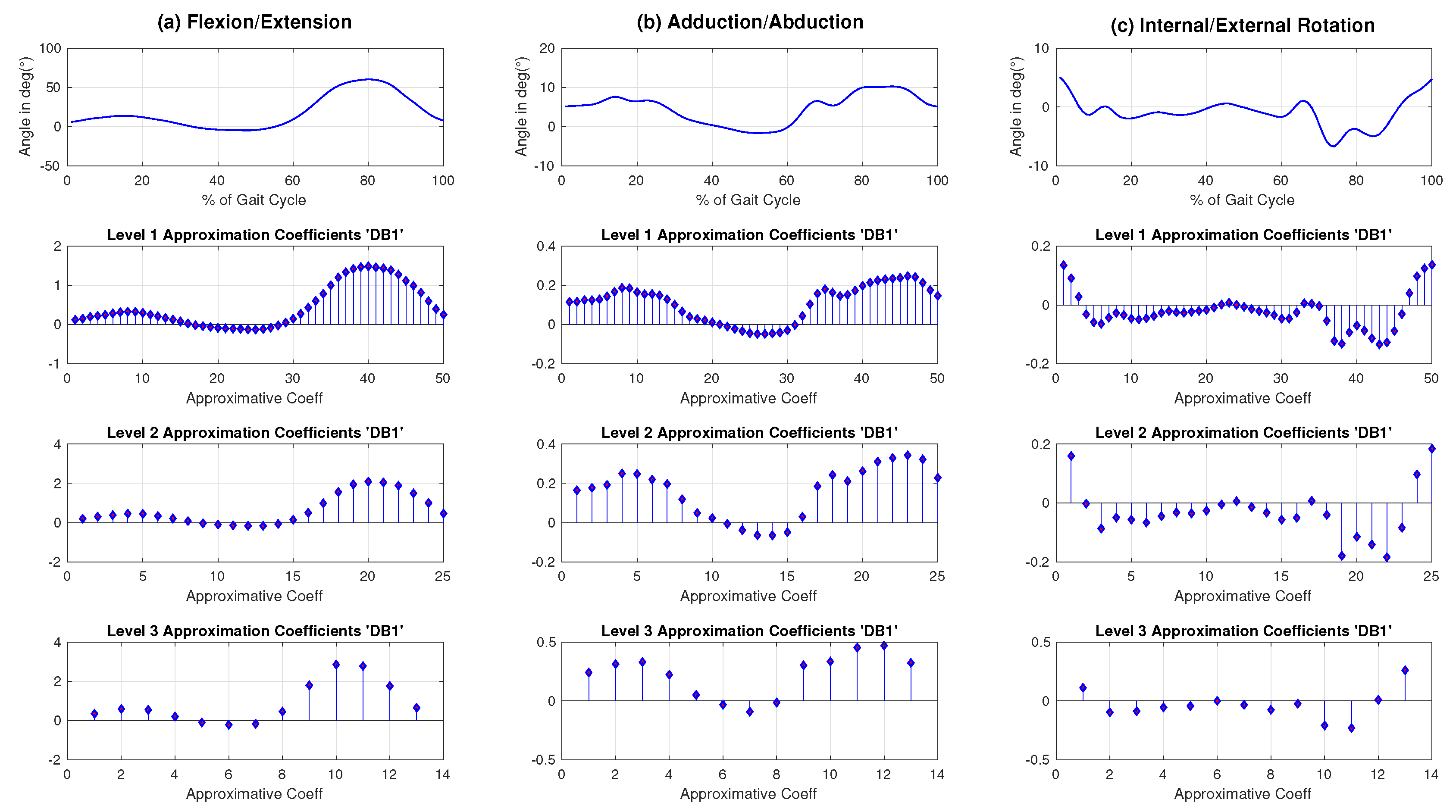
We experimented with different wavelet families, namely Daubechies, Coiflet, and Symlet. Figure 3 illustrates, for a randomly chosen participant’s curve, the wavelet coefficients using a Daubechies DB1 wavelet. The decomposition is performed on kinematic data in each plane separately: the flexion/extension angle, with respect to the sagittal plane (Figure 3a), the abduction/adduction angle, with respect to the frontal plane (Figure 3b), and internal/external angle, with respect to the transverse plane (Figure 3c).
The dimension of the data before feature extraction is 100, corresponding to the percentage of gait cycle (1% to 100%), for each of the three knee rotation angles. Using the wavelet decomposition for feature extraction, the dimension has been reduced to a lower number of coefficients. For instance, the wavelet decomposition using Daubechies DB1 at level 3 transforms the data dimension from 100 to 13 approximation coefficients (Figure 3, Line 4).
There are two main reasons for using a wavelet representation for feature extraction: (1) it has been effective for biomedical signal representation [33] and (2) it has the important property that it depends on the data to describe only, not on other data that enter the problem, in contrast to other common feature selection methods such as PCA and SVD [34].
We followed with the ReliefF ranking algorithm to determine the relevant wavelet coefficients from the obtained coefficients at the end of the decomposition procedure. The ranking has been performed on the extracted features on each plane separately and also on their concatenation. Following the ranking, we brought the extracted feature vector dimension to 12, i.e., the smallest sample size over all participants in the datasets which is the very first dimension reduction limit allowing the applicability of the Hotelling test.

4.3. Hotelling T 2 Test and Classification

The used software tools are from Matlab R2017b platform (Mathworks, Natick, MA, USA), and the T2Hot2iho routine of [35] for the two-sample, equal variance Hotelling test.
As introduced above, the first experiment uses dataset DS1 that contains data from 21 patients of the two classes C 1 and C 2 . Table 2 summarizes the classification rate for each plane separately and the best combination planes (Frontal and transverse). Using the wavelet decomposition for dimensionality reduction, the best Hotelling statistic test leave-one-out recognition rate (88.1%), on DS1 was achieved by the concatenation of seven approximation coefficients in a 3-level DB1 decomposition in the frontal plane and two approximation coefficients in a 6-level DB1 decomposition in the transverse plane. In this case, for each participant, the original data matrix is of (12×100) per plane (12 gait cycles × 100 points). Using a Daubechies DB1 at level 3 wavelet transformation in the frontal plane and a Daubechies DB1 at level 6 wavelet transformation in the transverse plane, the data matrix is reduced to (12 × 15) for each subject (12 gait cycles × 15 wavelet coefficients).
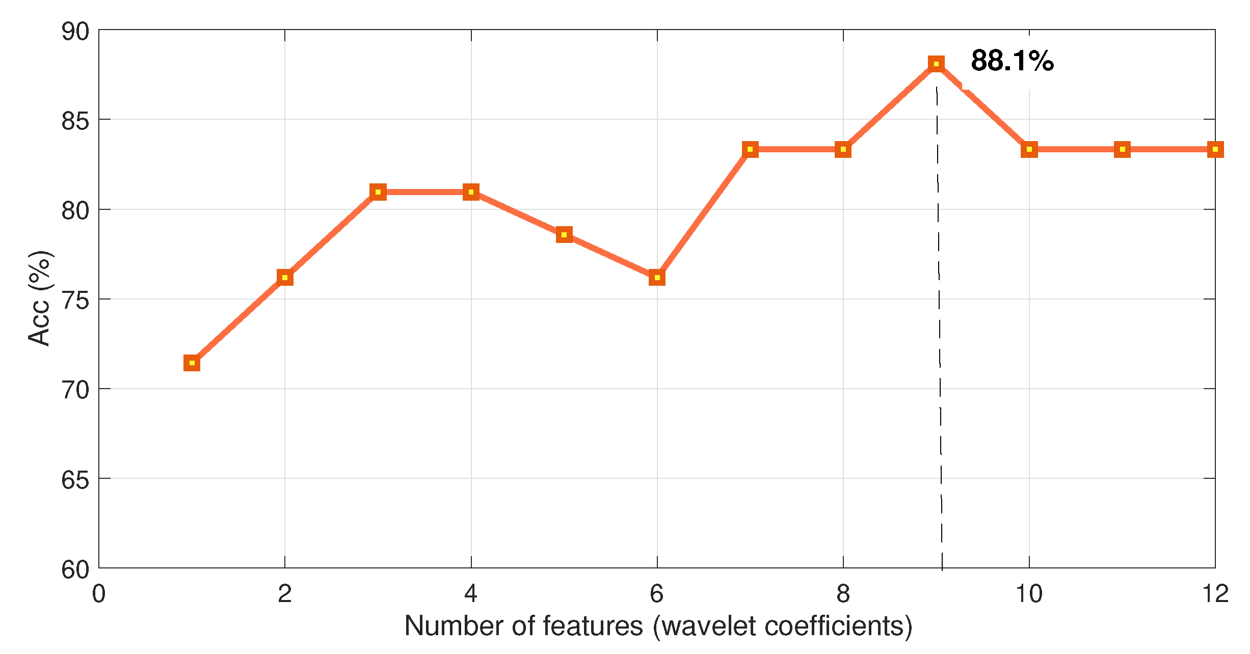
Figure 4 shows the classification accuracy according to the number of ranked features. We notice that the classification rate (Acc) reaches a maximum of 88.1%, using nine features, and then decreases as the number of features increases. This shows that feature selection algorithm can improve the accuracy of a classifier by using only relevant features, and also improve computational time as a result.
The confusion matrix corresponding to the Hotelling statistic classification on DS1 is given in Table 3. It shows which class is confused with which and at what rate ( τ C i ). The classification rates τ C i are balanced between the two classes C 1 (FR) and C 2 (FT) (19/21 (90.4%) in C 1 against 18/21 (85.7%) in C 2 ). For the much harder three-class problem, the second experiment considered three class classification, namely C 1 : FR, C 2 : FT, and C 3 : FR-FT. The method was able to obtain about 68.25 % correct decisions on DS2 using a leave-one-out procedure (Table 4). We note that the majority of confusion occurred with the class C 3 : FR-FT (22%, 14/63).
As one can expect, classification is much better on the two-class problem than on the three-class ( 88.1 % compared to 68.25 % ). This confirms the expectation that inclusion of class C 3 (FR-FT) adversely affects the problem difficulty in a significant way, indirectly confirming informal clinical assessments that considering class FR-FT, in addition to FR and FT, increases significantly the complexity of diagnosis.
For the three-class problem, which consists of distinguishing between FR, FT, and FR-FT, the method was able to obtain 68.25% correct decisions, justifying its further use and investigation. To the best of our knowledge, this study is the first to confront such a classification problem where both compartments (FR-FT) are affected by the presence of femero-rotulian osteoarthritis (FR) and femero-tibial osteoarthritis (FT).

4.4. Statistical Analysis

An analysis of variance was performed to verify the demographic characteristic group homogeneity. A post hoc Tukey test was used to examine the differences between pairs of groups. The implementation of this statistical processing was done via SPSS 20.0 (Statistical Package for Social Sciences). A p-value of 0.05 was set as the criterion for statistical significance.
The statistical analysis test confirms that there is no statistical difference between the demographic characteristics except between the age of C 1 and the other two classes. These results confirm that the classification performance is not influenced by the demographic characteristics.

4.5. Comparisons

Comparisons relate to different ways of representation of the knee kinematic data by dimensionality reduction and to different ways of classifying this data.

4.5.1. Dimensionality Reduction

For ways of data representation by dimensionality reduction, filter-based feature selection of wavelet coefficients is compared to principal component analysis (PCA), a common dimensionality reduction method. This comparison is in order to justify using a wavelet decomposition representation of the data, rather than a PCA representation. The PCA representation reduces the dimensionality by keeping only the variables that correspond to at least some fixed threshold of the total variation in the training data. Therefore, one eliminates the variables with no significant information for classification. In some cases, this can afford an important reduction of the dimensionality without affecting classification accuracy noticeably. However, PCA solutions are explicitly in terms of the training data, which makes them prone to artifacts, outliers, aberrations, and other such data non-representative of the underlying classes of the data [36].
The comparisons results show that the best result with PCA was obtained with the first two principal components, which maintained 67% of the data variance. The corresponding recognition rate was 59.52 % , compared to the 88.1 % , the best obtained with the Hotelling scheme and wavelet coefficient representation.

4.5.2. Classification

Duch [21] cites a large scale investigation that reviewed and compared the performance of several classifiers on several databases [37]. Although some classifiers, such as the nearest neighbors, appeared frequently among the best performers, the investigation found no systematic trend in the behavior of one classifier compared to the others: for each classifier, the results can be very good on some datasets but not on others. This is not too surprising because classification performance depends on the classifier, which itself relies on a model and its assumptions, as well as on the data representation, and the amount and layout of the learning data in the representation space. Investigations such as [37] legitimize the general practice in real world applications: seek the best classifier for the expected data inputs of a particular application rather than for data inputs at large. The choice of a particular classifier for an application is generally justified by the classifier better performance against the background of existing competing classifiers. Here, we will contrast the proposed Hotelling T 2 statistic method to commonly used classifiers of biomedical data [38], namely the K-nearest neighbor classifier (KNN), Linear discriminant analysis (LDA), and Support vector machine (SVM), a review and evaluation of which can be found in [39]. These methods, which can be potent, and their classification behavior, are also reviewed in pattern recognition textbooks, notably in classic Duda, Hart, and Stork [1]. Classification of OA data by these methods uses an average curve, or a single representative curve, rather than a sample, as a whole, of several measurement curves for each individual, to which it assigns a class membership according to a sample statistic such as Hotelling as in this study and [22]. This comparison will justify sample representation of data, used by the Hotelling classification scheme, against single vector representation used by others. We used Matlab routines to implement the KNN, LDA, and SVM classifiers. The routines are: KNN: ClassificationKNN.fit; LDA: fitcdiscr; SVM: templateSVM and fitcecoc.
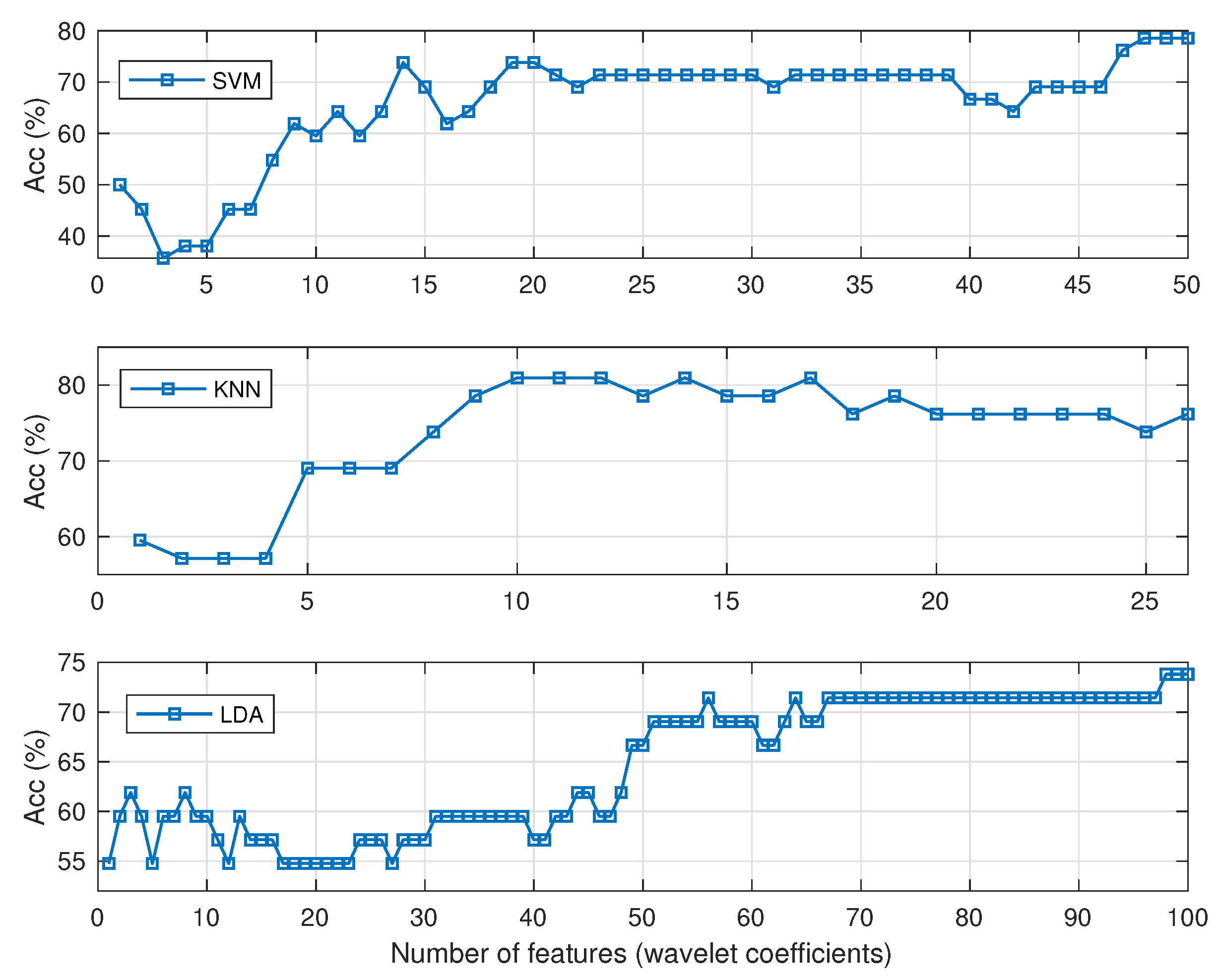
When the feature vector of data representation is the same for all the competing classifiers, then it is just a matter of running these classifiers and recording the various classification rates. However, when the feature vectors can vary with classifiers, as with the application in this study, the comparisons can be exceedingly laborious: for every classifier, the best possible score depends not just on the classification model but also on feature selection. Our study uses a wavelet representation of the original knee kinematic data curves. The wavelet coefficients of this representation are first ranked by the classifier-independent feature selection scheme ReliefF [40]. This type of scheme uses neighborhood feature differences to evaluate the relevance of features in describing each pattern class and, therefore, provide a way of ranking the features for subsequent selection to be included in the data representation. Selection looks for the combination of features that give the best classification performance: this is theoretically a combinatorial problem. Selection from a small set of ranked features is manageable: this is the case for the Hotelling statistic method proposed in this study, thanks to the fact that we needed to drop the dimension of the representation vector below a dozen, as explained earlier, for the Hotelling hypothesis testing to be applicable. For larger sets, it can be significantly more involved and exceedingly costly: this is the case for the three benchmark methods we used in the comparisons, namely LDA, KNN, SVM (we will refer to these as the benchmarks). We can nevertheless select good sets of features for these methods, as explained here in the following. First, we note that we are not constrained by any maximum number of features for the benchmarks. Therefore, it is legitimate to use the original kinematic data to determine which of the reference planes, or combination of planes thereof, is the most informative in that it gives the best recognition rate. Doing so gives the combination of the transverse and frontal planes as the best for SVM, KNN, and LDA (Table 5). This is the same best plane pair as for the Hotelling method. Assuming that the classifiers are all valid functions, this a reassuring result since it is then a property of the data that we are looking at. We can now proceed as with the Hotelling method: for each benchmark, use a multilevel wavelet decomposition of the data, rank the resulting coefficients using ReliefF, and select the combination of coefficients that yield the best recognition rate. However, the combinatorial dimension is excessive. Instead, we can have good features by selecting coefficients from the ranked coefficients at the best level of decomposition, which is level 3 (50 coefficients) for SVM, and 4 (25 coefficients) for KNN, and 1 (100 coefficients) for LDA (see Table 6). Doing so yields Figure 5, which shows the variation of the accuracy rate of each benchmark as a function of the number of selected coefficients expanded about the benchmark best decomposition level. The best performances are: SVM: 78 % with 48 coefficients, KNN: 81 % with 10 coefficients, and LDA: 74 % with 98 coefficients, placing the Hotelling method as a better performer at 88.1 % with nine coefficients.
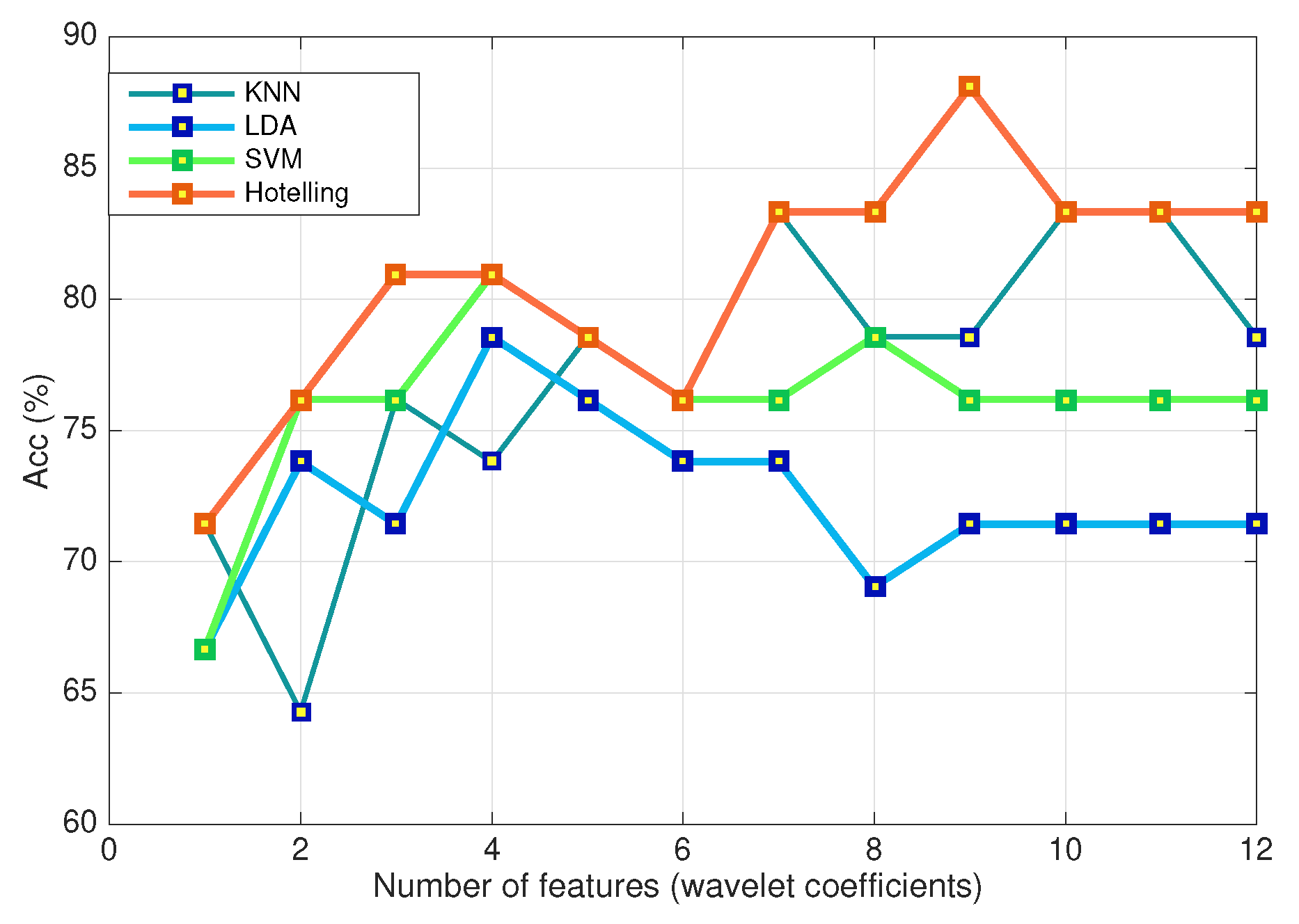
Another way to gain some insight into the comparative performance of the classifiers is to look at the behavior of the benchmarks running on a dozen coefficients as with the Hotelling statistic method. To do so, and to remain consistent with the treatment of the Hotelling method, we applied the same feature extraction and selection processing as described in Section Feature extraction and selection, i.e., the sample average curves have been reduced using a DB1 wavelet decomposition (seven approximation coefficients in a 3-level decomposition in the frontal plane and two coefficients in the transverse plane). The extracted features have been ranked with the ReliefF ranking algorithm.
The comparative recognition rates (Acc %) as a function of the number of features are shown in Figure 6. In almost all cases, the proposed Hotelling scheme gives a better recognition rate when tested on the dataset DS1. The results fit the expectation that using the average curve as input rather than the whole sample causes loss of information relevant to classification. In other words, averaging may suppress relevant information in the data which can be overcome when all the curves are retained for a more informative support to classification.
Ideally, one would be able to confirm the comparative experimentation conclusions by a run of all the methods on a validation database that has novel data, i.e., data yet unseen by any of the classifiers. In our case, unfortunately, we do not have such data, i.e., data that fits the application of OA pathology classification. Moreover, there are only 21 measurements for each pathology class (the small sample problem that the Hotelling method proposes to address), which is just too few to be able to cut out a portion to use as validation data.

5. Conclusions

The purpose of this study was to develop a classifier of three-dimensional kinematic data of knee movement that is reliable for small samples of high-dimensional data. The knee kinematic data come in the form of high-dimensional vectors representing the temporal variation of the three angles of rotation of the knee during locomotion. To address the notorious problems caused by high dimensionality and small sample sizes (the curse of dimensionality), the classifier used a Hotelling T 2 statistic on a reduced-dimensionality representation of the data.
In validation experiments, we applied the method to classify data in two classes of knee osteoarthritis pathologies, namely femero-rotulian (FR) and femero-tibilal (FT), and extended the application to three classes to include, in addition to FR and FT, category FR-FT representing the incidence of both diseases FR and FT in the same individual. The proposed method reaches an excellent 88.1 % correct classification rate for the two-class problem (FR and FT), improving significantly on the conventional classifiers. For the much harder three-class problem, to distinguish between FR, FT, and FR-FT, the method was able to obtain 68.25% correct decisions, justifying its further use and investigation. To the best of our knowledge, this study is the first to confront such a classification problem in spite of its importance.
As mentioned in the section on experimental comparisons, a comparative experimental analysis of the results obtained for a set of methods using on a train/test dataset, although informed, can be confirmed by an additional run of all the methods on a validation database that has novel data, i.e., data yet unseen by any of the methods’ classifiers. The results from such a validation run would offer more confidence in the generalization potency of the methods. In our case, unfortunately, we do not have proper data for this, i.e., data that would fit the application of OA pathology classification as used here. Moreover, there are only 21 measurements for each pathology class (the small sample problem highlighted in this study and that the Hotelling method proposes to address), which is just too few to allow cutting out a portion to use as validation data. Such a situation, not surprising in novel applications like ours, where data measurements are yet scarce, limits the generality of our comparative conclusions. The results obtained with the available data in this study justify further study of the Hotelling statistic classification method on new OA measurements of the sort we used, as well as its investigation with other biomedical data.
Author Contributions

Formal analysis, A.M., N.M., B.B.N., Y.O.; Methodology, B.B.N., N.M., A.M.; Writing—original draft, A.M., N.M.; Writing—review and editing, N.M., A.M.

Funding

This research was supported by the Natural Sciences and Engineering Research Council Grant, Industrial Research and Development Internship Program (RGPIN-2015-03853) and the Canada Research Chair on Biomedical Data Mining (950-231214).

Conflicts of Interest

The authors declare no conflict of interest.

References

  1. Duda, R.; Hart, P.; Stork, D. Pattern Classification; JohnWiley & Sons, INC.: Hoboken, NJ, USA, 2012. [Google Scholar]
  2. Martinez-Gonzalez, B.; Pardo, J.; Echeverry-Correa, J.; San-Segundo, R. Spatial features selection for unsupervised speaker segmentation and clustering. J. Experts Syst. Appl. 2017, 73, 27–42. [Google Scholar] [CrossRef]
  3. Lu, J.; Plataniotis, K.; Venetsanopoulos, A. Regularized discriminant analysis for the small sample size problem in face recognition. Pattern Recognit. Lett. 2003, 24, 3079–3087. [Google Scholar] [CrossRef]
  4. Kyperountas, M.; Tefas, A.; Pitas, I. Weighted piecewise LDA for solving the small sample size problem in face verification. IEEE Trans. Neural Netw. 2007, 18, 506–519. [Google Scholar] [CrossRef] [PubMed]
  5. Wang, J.; Plataniotis, K.; Lu, J.; Venetsanopoulos, A. Kernel quadratic discriminant analysis for small sample size problem. Pattern Recognit. 2008, 41, 1528–1538. [Google Scholar] [CrossRef]
  6. Yu, Y.; McKelvey, T.; Kung, S. A classification scheme for ‘high-dimensional-small-sample-size’ data using soda and ridge-SVM with microwave measurement applications. In Proceedings of the 2013 IEEE International Conference on Acoustics, Speech and Signal Processing, Vancouver, BC, Canada, 26–31 May 2013; pp. 3542–3546. [Google Scholar] [CrossRef]
  7. Krizhevsky, A.; Sutskever, I.; Hinton, G. ImageNet Classification with Deep Convolutional Neural Networks. In Proceedings of the 25th International Conference on Neural Information Processing Systems (NIPS’12); Curran Associates Inc.: Red Hook, NY, USA, 2012; Volume 1, pp. 1097–1105. [Google Scholar] [CrossRef]
  8. Frid-Adar, M.; Klang, E.; Amitai, M.; Goldberger, J.; Greenspan, H. Synthetic Data Augmentation using GAN for Improved Liver Lesion Classification. In Proceedings of the 2018 IEEE 15th International Symposium on Biomedical Imaging (ISBI 2018), Washington, DC, USA, 4–7 April 2018; pp. 1–5. [Google Scholar] [CrossRef]
  9. Hasan, C.Z.C.; Jailani, R.; Tahir, N.M. Automated Classification of Gait Abnormalities in Children with Autism Spectrum Disorders Based on Kinematic Data. Int. J. Psychiatry Psychother. 2017, 2, 10–15. [Google Scholar]
  10. Mezghani, N.; Ouakrim, Y.; Fuentes, A.; Mitiche, A.; Hagemeister, N.; Vendittoli, P.; De Guise, J. An Analysis of 3D Knee Kinematic Data Complexity in Knee Osteoarthritis and Asymptomatic Controls. PLoS ONE 2018, 13, 1–14. [Google Scholar] [CrossRef] [PubMed]
  11. Hunter, D. Focusing osteoarthritis management on modifiable risk factors and future therapeutic prospects. Ther. Adv. Musculoskelet. Dis. 2009, 1, 35–47. [Google Scholar] [CrossRef] [Green Version]
  12. Gaudreault, N.; Mezghani, N.; Turcot, K.; Hagemeister, H.; Boivin, K.; De Guise, J. Effects of physiotherapy treatment on knee osteoarthritis gait data using principal component analysis. Clin. Biomech. 2010, 26, 284–291. [Google Scholar] [CrossRef]
  13. Ben Nouma, B.; Mezghani, N.; Mitiche, A.; Ouakrim, Y. A variational method to determine the most representative shape of a set of curves and its application to knee kinematic data for pathology classification. In Proceedings of the 2nd Mediterranean Conference on Pattern Recognition and Artificial Intelligence (MedPRAI ’18), Rabat, Morocco, 27–28 March 2018; pp. 22–26. [Google Scholar] [CrossRef]
  14. Ben Nouma, B.; Mitiche, A.; Ouakrim, Y.; Mezghani, N. Knee kinematic curve representation and application to knee pathology classification. J. Biomed. Eng. Inform. 2018, 4, 32–39. [Google Scholar] [CrossRef]
  15. Mechmeche, I.; Mitiche, A.; Ouakrim, Y.; De Guise, J.; Mezghani, N. Data correction to determine a representative pattern of a set of 3D knee kinematic measurements. In Proceedings of the 2016 38th Annual International Conference of the IEEE Engineering in Medicine and Biology Society (EMBC), Orlando, FL, USA, 16–20 August 2016; pp. 884–887. [Google Scholar] [CrossRef]
  16. Zeng, W.; Ma, L.; Yuan, C.; Liu, F.; Wang, Q.; Wang, Y.; Zhang, Y. Classification of asymptomatic and osteoarthritic knee gait patterns using gait analysis via deterministic learning. Artif. Intell. Rev. 2018, 2, 1–19. [Google Scholar] [CrossRef]
  17. Koktas, N.; Yalabik, N.; Yauzer, G.; Duin, R.P. A multi-classifier for grading knee osteoarthritis using gait analysis. Pattern Recognit. Lett. 2010, 31, 898–904. [Google Scholar] [CrossRef]
  18. Mezghani, N.; Ouakrim, Y.; Fuentes, A.; Mitiche, A.; Hagemeister, N.; Vendittoli, P.; De Guise, J. Mechanical biomarkers of medial compartment knee osteoarthritis diagnosis and severity grading: Discovery phase. J. Biomech. 2017, 52, 106–112. [Google Scholar] [CrossRef] [PubMed]
  19. Hotelling, H. The Generalization of Student’s Ratio. In Breakthroughs in Statistics; Kotz, S., Johnson, N.L., Eds.; Springer: Berlin, Germany, 1992; pp. 54–65. [Google Scholar]
  20. Johnson, R.; Wichern, D. Applied Multivariate Statistical Analysis, 6 ed.; Prentice-Hall, Inc.: Upper Saddle River, NJ, USA, 2007. [Google Scholar]
  21. Duch, W. Similarity-based methods: A general framework for classification, approximation and association. Control. Cybern. 2000, 29, 1–30. [Google Scholar]
  22. Ben Nouma, B.; Mitiche, A.; Mezghani, N. A Sample-Encoding Generalization of the Kohonen Associative Memory and Application to Knee Kinematic Data Representation and Pathology Classification. Appl. Sci. 2019, 9, 1741. [Google Scholar] [CrossRef]
  23. McLachlan, G. Mahalanobis distance. Resonance 1999, 4, 20–26. [Google Scholar] [CrossRef]
  24. Daubechies, I. Ten Lectures on Wavelets; CBMS-NSF Regional Conference Series in Applied Mathematics: London, UK, 1992. [Google Scholar]
  25. Akanksha, N.; Mridu, S.; Shrish, V.; Vyom, R. Dimensionality Reduction for Motor Imagery Signal Classification using Wavelet Analysis. Int. J. Control. Theory Appl. 2017, 10, 65–76. [Google Scholar]
  26. Thepade, S.; Erandole, S. Extended performance comparison of tiling based image compression using wavelet transforms & hybrid wavelet transforms. In Proceedings of the 2013 IEEE Conference on Information & Communication Technologies, Tamil Nadu, India, 11–12 April 2013; pp. 1150–1155. [Google Scholar]
  27. Taujuddin, N.; Ibrahim, R.; Sari, S. Wavelet Coefficients Reduction Method Based On Standard Deviation Concept For High Quality Compressed Image. J. Theor. Appl. Inf. Technol. 2015, 79, 380–388. [Google Scholar]
  28. Boix, M.; Canto, B. Wavelet Transform application to the compression of images. Math. Comput. Model. 2010, 52, 1265–1270. [Google Scholar] [CrossRef]
  29. Rosario, S.F.; Thangadurai, K. RELIEF: Feature Selection Approach. Int. J. Innov. Res. 2015, 4, 218–224. [Google Scholar]
  30. Lustig, S.; Magnussen, R.; Cheze, L.; Neyret, P. The Knee KG system: a review of the literature. Knee Surg. Sports Traumatol. Arthrosc. 2012, 20, 633–638. [Google Scholar] [CrossRef]
  31. Hagemeister, N.; Parent, G.; Van de Putte, M.; St-Onge, N.; Duval, N.; De Guise, J. A reproducible method for studying three-dimensional knee kinematics. J. Biomech. 2005, 38, 1926–1931. [Google Scholar] [CrossRef] [PubMed]
  32. Labbe, D.; Hagemeister, N.; Tremblay, M.; de Guise, J. Reliability of a method for analyzing three-dimensional knee kinematics during gait. Gait Posture 2007, 28, 170–174. [Google Scholar] [CrossRef] [PubMed]
  33. Rafiee, J.; Rafiee, M.; Prause, N.; Schoen, M. Wavelet basis functions in biomedical signal processing. Expert Syst. Appl. 2011, 38, 6190–6201. [Google Scholar] [CrossRef]
  34. Prasad, S.; Bruce, L.M. Limitations of Principal Components Analysis for Hyperspectral Target Recognition. IEEE Geosci. Remote Sens. Lett. 2008, 5, 625–629. [Google Scholar] [CrossRef]
  35. Hotelling T-Squared Testing Procedures for Multivariate Samples. Available online: https://www.mathworks.com/matlabcentral/fileexchange/2844-hotellingt2 (accessed on 10 October 2018).
  36. Balsamo, L.; Betti, R.; Beigi, H. Damage detection using large-scale covariance matrix. In Proceedings of the Conference and Exposition on Structural Dynamics; Springer: Cham, Switzerland, 2014; Volume 5, pp. 89–97. [Google Scholar] [CrossRef]
  37. Rohwer, R.; Morciniec, M. A Theoretical and Experimental Account of n-Tuple Classifier Performance. Neural Comput. 1996, 8, 657–670. [Google Scholar] [CrossRef]
  38. Bishop, C.M. Pattern Recognition and Machine Learning; Elsevier: New York, NY, USA, 2012. [Google Scholar]
  39. Abid, M.; Mezghani, N.; Mitiche, A. Knee Joint Biomechanical Gait Data Classification for Knee Pathology Assessment: A Literature Review. Appl. Bionics Biomech. 2019, 2019, 7472039. [Google Scholar] [CrossRef] [PubMed]
  40. Kira, K.; Rendell, L. A Practical Approach to Feature Selection. In Proceedings of the Ninth International Workshop on Machine Learning (ML ’92), San Francisco, CA, USA, 1–3 July 1992; pp. 249–256. [Google Scholar] [CrossRef]
Figure 1. The functional diagram of the knee kinematic data classification system.
Make 01 00045 g001
Figure 2. The 12 samples of one participant (a) Flexion/Extension; (b) Abduction/Adduction; and (c) Internal/External Rotation.
Make 01 00045 g002
Figure 3. Wavelet decomposition using Daubechies DB1 (a) Flexion/Extension (Flex./Ext.); (b) Adduction/Abduction (Abd./Add.); and (c) Internal/External (Int./Ext.) knee rotation angle. Each line corresponds to a level of decomposition.
Make 01 00045 g003
Figure 4. Classification accuracy vs. number of features.
Make 01 00045 g004
Figure 5. Accuracy of the benchmarks as a function of the number of selected coefficients expanded about the best level of decomposition of each benchmark.
Make 01 00045 g005
Figure 6. Comparisons of classifier accuracies according to the number of retained relevant ranked features.
Make 01 00045 g006
Table 1. Demographic characteristics of the data in the three classes: columns FR, FT, and FR-FT.
Characteristics C 1 : FR C 2 : FT C 3 : FR-FT
Age (years)46.1 * ± 11.759.5 * ± 10.1 59.6 ± 11.4
Height(m) 1.71 ± 0.07 1.66 ± 0.09 1.66 ± 0.11
Weight (kg) 82.9 ± 20.7 76.2 ± 11.2 84.3 ± 15.9
BMI (kg/m 2 ) 28.3 ± 7.1 27.4 ± 3.9 30.3 ± 5.5
Men%4538 33.3
* indicate significant difference (p < 0.05).
Table 2. Feature selection and corresponding classification accuracy of the Hotelling statistic method on data in DS1 (classes FT and FR). The data planes are: sagittal(flexion/extension angle), frontal (abduction/adduction angle) and, transverse (internal/external angle).
PlanesLevelNumber ofNumber ofClassification
Extracted CoefficientsSelected Coefficients(Acc %)
Sagital54371.4
Frontal54478.6
Transverse47778.6
Frontal and transverse3 and 615 (13 and 2)9 (7 and 2)88.1
Table 3. The confusion matrix corresponding to the proposed Hotelling T 2 statistic classification on DS1.
Predicted C 1 : FR C 2 : FT τ C i ( % )
Actual
C 1 : FR19290.47 (19/21)
C 2 : FT31885.71(18/21)
Table 4. The confusion matrix corresponding to the proposed Hotelling T 2 statistic classification on DS2.
Predicted C 1 : FR C 2 : FT C 3 : FR-FT τ C i ( % )
Actual
C 1 : FR134461.90 (13/21)
C 2 : FT215471.42 (15/21)
C 3 : FR-FT601571.42 (15/21)
Table 5. Accuracies according to planes and plane combinations.
PlanesKNN (%)LDA (%)SVM (%)
Frontal67 (K = 1)7169
Sagittal43 (K = 1)5045
Transverse71(K = 3)5764
Frontal & Sagittal50 (K = 3)6957
Frontal &Transverse71 (K = 3)7476
Sagittal & Transverse48 (K = 3)5962
Frontal & Sagittal & Transverse62 (K = 5)6969
Table 6. Benchmarks’ accuracies according to levels of wavelet decomposition.
Level123456
Numb. of coefs.10050261484
SVM (%)767869626471
KNN (%)767676747472
LDA (%)747171696769