Abstract
In many statistical and machine learning applications, without-replacement sampling is considered superior to with-replacement sampling. In some cases, this has been proven, and in others the heuristic is so intuitively attractive that it is taken for granted. In reinforcement learning, many count-based exploration strategies are justified by reliance on the aforementioned heuristic. This paper will detail the non-intuitive discovery that when measuring the goodness of an exploration strategy by the stochastic shortest path to a goal state, there is a class of processes for which an action selection strategy based on without-replacement sampling of actions can be worse than with-replacement sampling. Specifically, the expected time until a specified goal state is first reached can be provably larger under without-replacement sampling. Numerical experiments describe the frequency and severity of this inferiority.
1. Introduction
The idea that learning is more efficient or estimates will be more precise when new, previously unseen information is processed has a strong intuitive appeal, and is often verified by theory. Consider the following elementary examples likely to be encountered by an undergraduate student. In sampling theory, consider estimating the mean of a collection of N values with variance by taking a sample of size . The variance of the sample mean when sampling with-replacement is , whereas the variance when sampling without-replacement is , which is strictly smaller for . For a probabilistic example, consider an urn with N marbles, exactly one of which is white. When searching for the white marble by drawing from the urn with-replacement, the number of draws is a geometric random variable and has expected value N. When searching by drawing without-replacement, the number of draws is a discrete uniform random variable and has expected value .
In more complex situations, it is generally difficult to analyze the behavior of without-replacement sampling due to the dependence between chosen items, so the argument in favor of without-replacement sampling or its variants is often made with numerical evidence. Examples include choosing ensemble classifiers [1], constructing low-rank approximations of large matrices [2,3], kernel embeddings [4], computational learning theory [5], and as a general purpose tool in evaluating data analysis applications [6]. A well-studied case is stochastic incremental gradient descent, for which there is a growing body of theoretical analysis [7,8,9,10] in favor of random reshuffling, which makes multiple passes through the data set, sampling without-replacement at each epoch.
Consider specifically the subdomain of reinforcement learning, in which an agent must learn how to behave optimally in an unknown Markovian environment [11]. Formally, the problem is cast as a Markov Decision Process [12], a sequential decision model in which a system can reside in one of a given set of states, S. At discrete points in time called epochs, the agent observes the state and chooses from among a set of actions, A. The system then transitions to the next state according to transition probabilities that depend on the current state and action, and a numeric reward is received. In the most general case, the reward is a random variable with a distribution that depends on the current state and action. The agent collects data by observing the state, choosing an action, and observing the resulting transition and reward. This data is used to construct a function from the state space to the action space, known as a policy , so that using action when in state s will optimize a given measure of reward.
In order to guarantee that the learned policy converges to the optimal policy, it is required that the number of observations goes to infinity [13]. In the case of discrete states and actions, each state–action pair must be observed an infinite number of times [14]. In the case of continuous states and actions, the distribution of observed states and actions must have a density that is positive everywhere [15]. A practical corollary is that for an algorithm to learn well from a finite amount of data, this data should contain observations that represent the state-action space as completely as possible. Therefore, a key component of a reinforcement learning algorithm is how they explore, that is, how actions are chosen so that the data has enough variety for meaningful learning.
Exploration in reinforcement learning has been, and remains, an active research topic since the inception of the field. Some of the most common strategies include -greedy [16], in which the agent chooses the best known action with probability and a random action with probability ; softmax exploration [17], in which a distribution (usually the Boltzmann distribution) links the probability of selecting an action to its estimated value; “optimism in the face of uncertainty” [18], which assumes that actions with unknown or uncertain rewards are better than known actions, encouraging their use by a greedy agent; and statistical approaches such as maintaining a confidence interval for the value of each state-action pair, and choosing the action with the greatest upper confidence bound [19]. Another class of exploration strategies keeps a history of the actions used in each state. Upon visiting a state, recency-based exploration [20,21] incentivizes the use of actions that have not been recently used from that state, which is especially helpful for continued learning in changing environments. Similarly, count-based exploration [22,23,24] incentivizes actions that have been used less frequently.
Of particular interest to this paper is a count-based strategy used by Kearns and Singh [25] in their “Explicit Explore or Exploit” () algorithm. This algorithm is notable for achieving near-optimal performance in a time with a proven polynomial bound. The “Explore” part of the algorithm is a simple yet appealing strategy that the authors call balanced wandering. Under this strategy, a record is kept of how many times each action has been used for each state. When a state is visited, the action is chosen uniformly from among the actions that have been used in that state the least number of times. Note that this is equivalent to the random reshuffling used in without-replacement stochastic incremental gradient descent, but on a per-state basis. Upon subsequent visits to a particular state, actions will be sampled without-replacement until all actions have been tried, at which point sampling begins anew.
There are several reasons to believe that balanced wandering may provably be a uniform improvement over exploration using purely random, with-replacement action selection. First, balanced wandering is a relatively simple exploration strategy which has already been proven amenable to theoretical analysis [25]. Second, it can be viewed as an application of random reshuffling to reinforcement learning, which has been proven to be an improvement for stochastic gradient descent. Third, as argued in the opening paragraph, the intuition that without-replacement sampling yields more and better information than with-replacement sampling is undeniably strong.
The research presented in this paper is the result of an investigation initially intending to prove that balanced wandering is uniformly superior to with-replacement sampling of actions. However, we were surprised to discover that the hypothesis in general is false, and there exists a class of Markov decision processes for which balanced wandering is worse in terms of expected time until a goal state is reached. The latter half of the project then became a search for understanding how this seeming paradox can occur, and finding a counter-proof to the hypothesis that balanced wandering is always superior.
The remainder of this paper is organized as follows. Section 2 sets up the mathematical preliminaries, describes the two exploration strategies under investigation, defines the metric by which they are compared, and states the hypothesis under investigation. Section 3 proves that for the smallest decision processes, balanced wandering is indeed a strict, uniform improvement over with-replacement action selection. Section 4 finds and proves conditions on transition probabilities that are sufficient for balanced wandering to be worse, and presents an intuitive explanation as to how the paradox may occur. Section 5 contains the result of a numerical experiment to investigate the frequency and magnitude of the paradox. Section 6 concludes with ideas for future research.
2. Preliminaries
Throughout this paper, N will denote the number of states and M the number of actions of a Markov Decision Process (hereafter MDP). Let be a finite set of states in which the system may reside. Let state 1 be an initial state the system begins in, and state N a goal state the agent is trying to reach. Let be a finite set of actions from which the agent may choose. Associated with each state-action pair is a probability distribution on the states, , which governs the transition to the next state. For example, denotes the probability of transitioning to state j when action k is used from state i. The transition probabilities are assumed to be stationary in time and have the Markov property: they are conditionally independent of past states and actions given the current state and action.
MDPs typically include a reward received at each epoch. This paper focuses on the exploration portion of the learning problem, so rewards can be ignored. If this bothers the reader, we suggest supposing that all states emit a reward of zero except for the goal state N, which emits a positive reward. This would be pertinent to a learning algorithm for a process with a single reward state; no meaningful learning can take place until the first epoch at which a state with a positive reward is encountered, so it is desirable to find a state with positive rewards as quickly as possible.
Consider the following two methods for selecting actions from a finite set:
- Random Action Selection (hereafter denoted RAS): Whenever a state is visited, the agent chooses the action randomly and uniformly from the set of all actions.
- Balanced Wandering (hereafter denoted BW): For each state, a history is kept of the number of times each action has been tried. Whenever a state is visited, the agent inspects the history of actions tried from that state, and creates a subset of the actions that have been tried the least number of times. The agent chooses the action randomly and uniformly from the actions in that subset.
There is an equivalent formulation of BW which will be helpful in a forthcoming analysis. Notice that under BW, for a given state and any positive integer n, each action must be tried n times before any action can be tried times. Then, as M represents the number of actions, each state is initially assigned a random permutation of the M actions to be executed in the first M visits to that state. After visit M, a new random permutation of the M actions is assigned to the next M visits to that state, and so on.
Define and to be the hitting times for the goal state, that is, the first time at which the system reaches state N, under each exploration strategy. That is,
In Section 3 and Section 4, we assume that state N is accessible from all states, so . Because the state space is finite, standard Markov chain theory implies . In Section 5, we will consider the possibility of an absorbing class of states or dead ends [26] from which the goal state cannot be reached.
Hypothesis 1.
For an MDP with an arbitrary number of states N and arbitrary number of actions M, the expected hitting time for the goal state under BW is less than or equal to the expected hitting time for the goal state under RAS. That is,
The following two sections will show that this hypothesis is true for states, but false in general for .
By using expected hitting time to measure the effectiveness of an exploration strategy, we are essentially casting the problem as a special case of a stochastic shortest path (SSP) scenario [27]. An SSP is a type of MDP, often considered as a weighted directed graph, with the goal of selecting actions so that the journey from an initial state to a target state has the minimum possible expected sum of weights for traversed edges. Because we are seeking the strategy with expected minimum hitting time, this corresponds to an SSP where each edge is the transition time between states, so all edges have a weight of one.
3. A Proof for
Consider the simple MDP which consists of a finite state space and a finite action space . Let state 1 be the initial state of the system, and state 2 be the goal state. Then, is the random variable denoting the number of epochs until the first time the system transitions to state 2. Similarly, denotes the number of epochs until first reaching state 2 under BW.
Before stating and proving the theorem, we review some established definitions and results that will be needed in the proof.
Definition 1.
Let be real numbers. For integer , the elementary symmetric polynomial of degree k in , denoted , is the sum of all products of k distinct elements from . That is,
for . It is the sum of terms, where each term is the product of an unordered sample without-replacement of size k. The polynomials corresponding to and are the sum of the terms and the product of the terms respectively, and .
Definition 2.
The elementary symmetric mean of degree k of , denoted , is the mean of the terms in the elementary symmetric polynomial of the same degree.
Notice that is the arithmetic mean, and is the geometric mean raised to the power n.
Theorem 1
(Maclaurin Inequality). For ,
Furthermore, the inequalities are strict unless .
See Biler [28] for a proof. Notice that this is a refinement of the well-known inequality between the arithmetic mean and the geometric mean, which can be recovered by comparing the first and last terms in the sequence of inequalities. Theorem 2 can now be proved.
Theorem 2.
For a two-state MDP,
This inequality is strict unless every action has an equal probability of transitioning to state 2.
Proof.
The first step is recognizing that tail probabilities for the hitting times can be expressed as elementary symmetric means of the transition probabilities under each action. For compactness of notation, denote the probability of transitioning from state 1 to state 2 using action m by , and the probability of remaining in state 1 under action m by . First, consider RAS. Because every action has probability of being chosen, the overall probability of transitioning from state 1 to state 2 is given by the Law of Total Probability as
which is simply the average of the probabilities of transitioning from state 1 to state 2 under each action. Then , the number of epochs until the first successful transition under random action selection, is a geometric random variable with parameter , and has tail probabilities
Now consider tail probabilities under BW. Recall that this action selection scheme is equivalent to assigning a permutation of the M actions to each state to be executed sequentially. For a value , the event means that the first k actions that were tried did not result in a successful transition to state 2. Partitioning this event according to the first k actions in the permutation and applying the Law of Total Probability shows that this probability can also be expressed in terms of elementary symmetric means. Let denote the set of all combinations of k integers out of the first M integers, representing the first k actions used. Each combination of k actions is equally likely, so the probability of each set in the partition is . Formally,
A direct application of the Maclaurin Inequality shows that, for ,
The next step is to use this inequality to obtain an inequality between conditional expectations for the hitting times.
For the conditional expectation , notice that after epoch M every action has been tried exactly once, and the state receives a new permutation of the M actions to execute in the following M time steps. Hence, if the system has not transitioned to state 2 by M time steps, then the process probabilistically restarts. For RAS, this is actually true at every time step, but under BW this only occurs at multiples of M. This yields the expressions
Finally, consider the unconditional expectation under each action selection scheme.
Solve this expression for .
The same logic is used to show
A term-by-term comparison shows that , which completes the proof. □
4. A Counter-Proof for
The argument used in the preceding proof does not extend to states. After several other proof strategies also failed, we began to wonder if the hypothesis is true in general. This section states and proves conditions that show analytically Hypothesis 1 is false in general. Because there are now an arbitrary number of states, we return to the general notation for transition probabilities, in which represents the probability of transitioning to state j when action k is used from state i. First, a quantity is defined which will be useful in the proof.
Definition 3.
Let . Define to be the average probability of transitioning from the initial state to the goal state if action m is excluded. That is,
Theorem 3.
Consider an MDP with states and an arbitrary number of actions M.
Before starting the formal proof, see that Equation (2) has an interpretation that helps with an intuitive understanding of how the paradox may happen. BW is inferior relative to RAS when the left side is large, which happens when the actions having the greatest probability to transition directly from the initial state to the goal state also are likely to remain in the initial state. Therefore, if the use of one of these actions results in the system remaining in the initial state, it would be desirable to use the same action again. Under RAS, it is possible to use the same action from the initial state multiple times in a row, but BW forces the use of other, inferior actions. When this effect is large enough, .
Proof.
A well-known fact from probability theory states that the expected value of a non-negative integer-valued random variable X can be found as a sum over tail probabilities, ([29], p.3). Applying this to the hitting times under RAS and BW, we have
Notice that the first two differences in the sum are zero and have been dropped. For , both tail probabilities are one. For , using the rule of complements, because all actions are available, thus the probabilities of transitioning directly to the goal are equivalent. Then, moving the term out of the sum,
The strategy will be to choose transition probabilities so that the left side is positive and large, and the right side has a small absolute value. Consider first the left side. Elementary but tedious calculations, which are deferred to the Appendix A, show that
Now consider the right side. Assumption (1) says that no matter what the current state and action are, there is always a probability of at least c of transitioning directly to the goal. Therefore, and are each strictly less than , as is the absolute value of their difference. Using this with well-known formulas for sums and partial sums of geometric series, we obtain
Combining the expressions for the left and right sides, we see that Equation (2) is sufficient for . It still remains to show existence; that there are probabilities and a value of c satisfying Equations (1) and (2)). Now consider the MDP with probabilities defined in Equation (3). Clearly, these probabilities satisfy Equation (1). The left side of Equation (2) only has one non-zero term, so combining with , it can be simplified as follows:
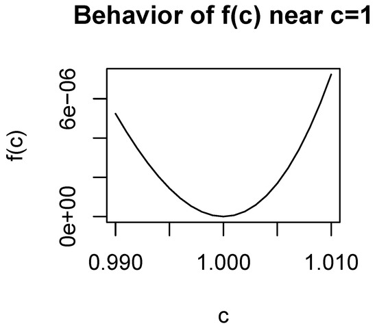
It remains to show there is a value such that
Call the left hand side . Note that . Find first and second derivatives at :
A continuous function with and is necessarily positive for some value . Figure 1 illustrates this by plotting in a neighborhood of one when . This completes the proof. □
Figure 1.
The behavior of near for . when , for which a neighborhood exists for values of c just below 1.
5. Numerical Experiments
Now that Hypothesis 1 is known to be false in general, several questions are immediately raised.
- How often is ? If an MDP is randomly generated, what is the probability BW will be worse than RAS for reaching the goal state?
- How much worse can BW be than RAS? Does this depend on N and M?
- For a randomly generated MDP, the difference can be regarded as a random variable. What are the characteristics of the density of the difference?
- If we allow the existence of dead ends so that the goal state is not accessible from all states, can Hypothesis 1 still be violated?
This section explains how we investigate answers to these questions via numeric calculation of and for randomly generated MDPs.
First, we need a procedure for constructing a random MDP, which essentially reduces to repeatedly generating discrete distributions where the probabilities are themselves random. This is accomplished by generating independent uniform random variables, and standardizing so that they sum to one. Algorithm 1 gives pseudocode for this procedure, which the reader can find implemented in the language R [30] in the Supplementary Material as the function makeProbArray().
| Algorithm 1: Pseudocode for randomly generating the probabilities for an MDP with a specified number of states and actions. |
 |
Once the transition probabilities are generated, finding is straightforward. Under RAS, the system is an ordinary Markov chain with transition probabilities
Finding the expected hitting time for a specified state in a Markov chain is a standard technique (see, for example, Section 2.11 of Resnick [29]) and so is stated without derivation. Force the goal state N to be absorbing by setting and for . Let Q be the matrix containing transition probabilities between transient states, I the identity matrix of the same size as Q, and a column vector of all ones with the same number of rows as Q. Then,
is a vector with entry k containing the expected time until absorption starting from state k. Therefore, is found as the first entry. In the Supplementary Material, this is implemented in the function expectedHittingTimeRAS()
Finding is less straightforward. The process under BW is not a Markov chain because transition probabilities depend on which actions are available from which state, which depends on actions used in the past. However, the Markov property can be recovered by including enough information about the history of used actions in the state space. We call the resulting process the induced MDP, in contrast with the original MDP, and will now detail its construction.
Definition 4.
Let N and M be the number of states and actions respectively in the original MDP. A history matrix H is an binary matrix with the restriction that a row cannot consist entirely of ones. The set of all history matrices is denoted by .
An entry of one in row i and column j of H indicates that action j has already been used in the current permutation of actions for state i, therefore action j is currently unavailable from state i. Likewise, an entry of zero in row i and column j means action j is available from state i. The restriction that a row cannot consist entirely of ones corresponds to BW assigning a new permutation of actions once the current pass has ended, meaning the row would consist entirely of zeros.
For example, for the following history matrix, if the system is in state 1, then action 2 must be used, at which point the first row reverts to all zeros. If the system is in state 2, action 1 must be used, and the second row resets. If the system is in state 3, actions 1 and 2 are eligible, so each action has a 50% chance of being selected. The entry in the third row for the chosen action would change to 1.
The state space for the induced process is ; that is, for the Markov property to hold, one must know both the state from the original process and information about the actions used from each state. The number of states in is much larger than the number of states in S. There are possibilities for each row of the history matrix, and there are N rows, so there are possible history matrices. Finally a state in must also include one of the N states from S, so there are states total in .
Now we define transitions between states in the induced process. Let , and , so that . First recognize that it will not be possible to transition from to in one epoch unless the history matrix for the second state reflects the most recently used action but is otherwise identical to the history matrix from the first state. This motivates the following definition.
Definition 5.
Let , and . We say that is m-compatible with if has an entry of zero in row i and column m, and changing that entry to a one results in .
Intuitively, m-compatibility means that action m is available to be selected from the current state, and that is the resulting history matrix when action m is used (remembering the possibility that if this causes row i to consist entirely of ones, it resets to a row entirely of zeros).
Let be the number of entries in row i of that are equal to zero. That is, is the number of actions available to choose from when in state i. Then, transition probabilities in the induced process are defined by
Equation (7) can be understood in three parts. First, the requirement that induced states are compatible ensures that the history matrix is properly updated. Second, the denominator accounts for the number of actions available to choose from. Third, the numerator accounts for the transition probabilities from the original MDP. In the Supplementary Material, the construction of the transition matrix in the induced MDP is implemented in the function makeInducedChain(). Once the transition matrix is obtained, the submatrix corresponding to transitions between transient states can be extracted, and finally can be obtained from the calculation in Equation (6). These final steps are implemented in the function expectedHittingTimeBW().
The results of the numerical investigation are presented in Figure 2. For each combination of values of N and M, Algorithm 1 was used to generate 1000 MDPs. Notice that because the size of the induced state space grows so rapidly with N and M, results are only given for . For , our hardware could not complete the experiment in a reasonable amount of time.
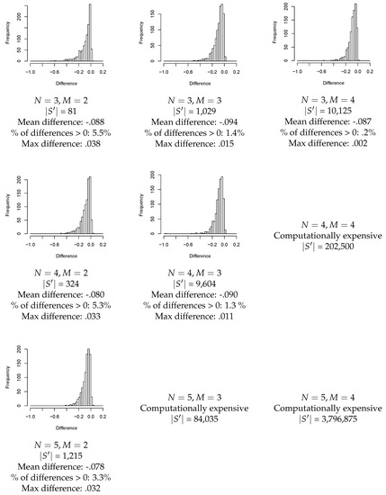
Figure 2.
Results of numerical experiments calculating for randomly generated Markov Decision Processes (MDPs). In total, 1000 MDPs were generated for each combination of N and M.
For each MDP, the difference was calculated. The figure displays a histogram of the differences, which all share commonalities. The peak is consistently slightly less than zero, indicating that typically RAS is slightly better than BW. The distribution has a left skew, so there are MDPs for which RAS is significantly better. Finally, very little of the distribution is to the right of zero, so while Hypothesis 1 can be false, it is rare and BW is not worse by a large degree.
In addition to the histograms, Figure 2 gives the mean difference, the percentage of differences that are greater than zero (signifying how often Hypothesis 1 is false), and the maximum observed distance, giving a sense of how strongly Hypothesis 1 can be violated. The mean difference is consistently close to , and deviations are small relative to the sampling error, so there is little evidence that the mean difference changes substantially with N and M. On the other hand, the percentage of positive differences and the maximum difference appear to decline slightly as N, the number of states increases, and decline sharply as M, the number of actions increases. Therefore, it seems that the frequency and magnitude of violations of Hypothesis 1 decrease as the MDP becomes more complex.
Until now, we have assumed that no matter what state the system is in, the goal state is accessible. That is, there is always a sequence of states and actions with a positive probability of reaching the goal. In many real life applications, the system may enter a dead end [26], which is a state from which it is impossible to reach the goal. If such states are allowed, then the SSP implicitly becomes a multi-objective optimization problem [31], as the agent must simultaneously try to avoid the dead ends while still minimizing the expected cost of reaching the goal.
In this investigation, we handle dead ends by allowing the system to reset to the initial state, but with a penalty of additional time to do so. Formally, this is implemented by adding a return state, R. If the system enters a dead end, it will transition to the return state with probability one, and then transition to the initial state with probability one, at which point the search for the goal state begins anew.
This modification can be observed in the following example. The matrix on the left represents the transition probabilities under an arbitrary action, with state 2 being absorbing. If state 2 is absorbing for all actions, then state 2 is a dead end. On the right, the matrix has been modified so that state 2 leads to the return state R.
As mentioned previously, the state space for the induced process under BW grows rapidly, and exact calculation of the expected hitting time rapidly becomes infeasible. This is even more so when dead ends are allowed, as the additional return state increases the size of the induced process. For this reason, we could not replicate the entire experiment shown in Figure 2 allowing dead ends, but we did discover that processes still exist for which BW is worse than RAS. Figure 3 gives an example of such a process, and code for reconstructing it is in the Supplementary Material.
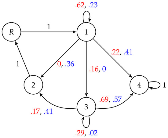
Figure 3.
An example of an Markov Decision Process (MDP) with a dead end for which . The first and second values on each edge, in red and blue, are the transition probabilities under actions 1 and 2 respectively. Edges with a single weight, in black, are irrespective of actions. Note that state 2 is a dead end, and returns to the initial state after passing through the return state. For this example, and .
6. Conclusions
This paper has compared two strategies for exploring Markov decision processes with the goal of reaching a specified state in the shortest average number of epochs. Though intuition suggests that the strategy using without-replacement sampling of actions would be uniformly superior, we have shown that this is only true for processes with two states.
As with most non-intuitive discoveries, more questions are raised than answered, and there are many avenues for possible future research. Some of these questions are addressed here.
How can behavior under BW be efficiently investigated when the number of states and actions is large? The state space of the induced process grows rapidly, and it soon becomes impractical to use the standard method for calculating the expected hitting time which requires inversion of the transition matrix. We have also attempted to estimate the hitting time statistically by repeated simulation, but the sampling variance is large relative to the difference , making it difficult to have confidence in any inferences. Further investigation will require the application or development of techniques beyond those used in this paper.
Though it is difficult to analyze large processes exactly, we can make a conjecture. From the numerical experiments, it seems that the difference between RAS and BW (in terms of the percentage of times BW is worse and the maximum degree by which RAS is better) decreases as the number of actions increases. An insight gained from Equation (2) gives reason to believe that this may be true. The term , the probability of transitioning when action m is unavailable, is key. However, as the number of actions increases, will necessarily differ little for each value of m. This corresponds to the notion that sampling with and without replacement become more similar as the number of elements that can be sampled increases. Therefore, we conjecture that the phenomena studied in this paper will be less relevant for larger processes.
Is the use of count-based exploration practically harmful in any state-of-the-art applications? This has not yet been investigated. For future research, the authors intend to implement each of RAS and BW as exploration strategies in benchmark problems and see if the behavior learned is significantly different.
Are there other measures beyond expected hitting time for which BW can be proven strictly better? By using the expected hitting time criteria for a single goal state, we are admittedly limiting ourselves to the study of stochastic shortest path MDPs. Perhaps a more complete metric would be the performance of an agent trained on the data collected by each exploration strategy. This type of analysis is deferred for future research.
In Theorem 3, Equation (1) explicitly requires the goal be accessible from all states, so the same proof strategy cannot be extended to processes with dead ends. Computations also become more difficult with dead ends. At this point, we know that Hypothesis 1 can still be violated when dead ends exist, but nothing else is known for certain. Dead ends provide another avenue for future research.
Theorem 3 is essentially an existence proof which finds sufficient conditions for Hypothesis 1 to be false; can it be extended to finding necessary conditions as well, providing a complete characterization? There is still much work to be done before a complete understanding of optimal exploration in Markovian environments is reached.
Supplementary Materials
The following are available online at https://www.mdpi.com/2504-4990/1/2/41/s1, Script S1: A script in the language R containing functions for implementing the numeric experiments.
Author Contributions
Conceptualization, S.W.C.; investigation, S.W.C. and S.D.W.; writing—original draft preparation, S.W.C.; writing—review and editing, S.W.C. and S.D.W.
Funding
This research received no external funding.
Acknowledgments
The authors are grateful to the anonymous reviewers for their suggestions regarding stochastic shortest paths and dead ends.
Conflicts of Interest
The authors declare no conflict of interest.
Abbreviations
The following abbreviations are used in this manuscript:
| MDP | Markov Decision Process |
| SSP | Stochastic Shortest Path |
| RAS | Random Action Selection |
| BW | Balanced Wandering |
Appendix A. Proof of Equation (5)
A hitting time greater than two means that the goal state was not reached in the first two transitions. Consider all possible combinations of states and actions that do not reach the goal in the first two epochs. There are three categories:
- Paths that transition away from the initial state at the first epoch.
- Paths that stay in the initial state, but use a different action on the second epoch.
- Paths that stay in the initial state, but use the same action on the first two epochs.
Under RAS, any path is possible, with the probability of a path being the product of the probability of choosing the actions (which is always ) and the transition probabilities between states. Thus partitioning according to the categories described above,
Under BW, paths in the first category have the same weighting as under RAS. However, paths in the second category have a weight of because the action used at the first time step cannot be used again from the initial state, so the probability of choosing any specific action for the second time step is . Furthermore, paths in the third category are not possible under BW, thus
When the difference is taken, the probabilities for paths in the first category will cancel. The index is no longer used, so the subscript on can be dropped without ambiguity.
Obtain a common denominator of so that the quantities can be combined. This will introduce a in the numerator of the third quantity, which will disappear when it is absorbed into the sum over .
From the rule of complements, for any action m. Apply this to the previous expression. Then
as desired.
References
- Pathical, S.; Serpen, G. Comparison of subsampling techniques for random subspace ensembles. In Proceedings of the 2010 International Conference on Machine Learning and Cybernetics, Qingdao, China, 11–14 July 2010; Volume 1, pp. 380–385. [Google Scholar] [CrossRef]
- Kumar, S.; Mohri, M.; Talwalkar, A. Sampling Methods for the Nyström Method. J. Mach. Learn. Res. 2012, 13, 981–1006. [Google Scholar]
- Williams, C.K.I.; Seeger, M. Using the Nyström Method to Speed Up Kernel Machines. In Advances in Neural Information Processing Systems 13; Leen, T.K., Dietterich, T.G., Tresp, V., Eds.; MIT Press: Cambridge, MA, USA, 2001; pp. 682–688. [Google Scholar]
- Schneider, M. Probability Inequalities for Kernel Embeddings in Sampling without Replacement. In Proceedings of the 19th International Conference on Artificial Intelligence and Statistics, Cadiz, Spain, 9–11 May 2016; Volume 51, pp. 66–74. [Google Scholar]
- Cannon, A.; Ettinger, J.M.; Hush, D.; Scovel, C. Machine Learning with Data Dependent Hypothesis Classes. J. Mach. Learn. Res. 2002, 2, 335–358. [Google Scholar]
- Feng, X.; Kumar, A.; Recht, B.; Ré, C. Towards a Unified Architecture for in-RDBMS Analytics. In Proceedings of the 2012 ACM SIGMOD International Conference on Management of Data, SIGMOD’12; ACM: New York, NY, USA, 2012; pp. 325–336. [Google Scholar] [CrossRef]
- Gürbüzbalaban, M.; Ozdaglar, A.; Parrilo, P. Why Random Reshuffling Beats Stochastic Gradient Descent. arXiv 2015, arXiv:1510.08560, [arXiv:math.OC/1510.08560]. [Google Scholar]
- Meng, Q.; Chen, W.; Wang, Y.; Ma, Z.M.; Liu, T.Y. Convergence analysis of distributed stochastic gradient descent with shuffling. Neurocomputing 2019. [Google Scholar] [CrossRef]
- Ying, B.; Yuan, K.; Vlaski, S.; Sayed, A.H. Stochastic Learning Under Random Reshuffling with Constant Step-sizes. IEEE Trans. Signal Process. 2019, 67. [Google Scholar] [CrossRef]
- Shamir, O. Without-Replacement Sampling for Stochastic Gradient Methods. In Advances in Neural Information Processing Systems 29; Lee, D.D., Sugiyama, M., Luxburg, U.V., Guyon, I., Garnett, R., Eds.; Curran Associates, Inc.: Red Hook, NY, USA, 2016; pp. 46–54. [Google Scholar]
- Sutton, R.S.; Barto, A.G. Introduction to Reinforcement Learning, 1st ed.; MIT Press: Cambridge, MA, USA, 1998. [Google Scholar]
- Puterman, M. Markov Decision Processes: Discrete Stochastic Dynamic Programming; Wiley Series in Probability and Statistics; Wiley-Interscience: Hoboken, NJ, USA, 2005. [Google Scholar]
- Tsitsiklis, J.N.; Roy, B.V. An Analysis of Temporal-Difference Learning with Function Approximation. IEEE Trans. Autom. Control 1997, 42, 674–690. [Google Scholar] [CrossRef]
- Watkins, C.J.C.H.; Dayan, P. Q-learning. Mach. Learn. 1992, 8, 279–292. [Google Scholar] [CrossRef]
- Carden, S.W. Convergence of a Q-learning Variant for Continuous States and Actions. J. Artif. Intell. Res. 2014, 49, 705–731. [Google Scholar] [CrossRef]
- Wunder, M.; Littman, M.; Babes, M. Classes of Multiagent Q-learning Dynamics with ϵ-greedy Exploration. In Proceedings of the 27th International Conference on Machine Learning, Haifa, Israel, 21–24 June 2010; pp. 1167–1174. [Google Scholar]
- Tijsma, A.D.; Drugan, M.M.; Wiering, M.A. Comparing exploration strategies for Q-learning in random stochastic mazes. In Proceedings of the 2016 IEEE Symposium Series on Computational Intelligence (SSCI), Athens, Greece, 6–9 December 2016; pp. 1–8. [Google Scholar] [CrossRef]
- Kaelbling, L. Learning in Embedded Systems. Ph.D. Thesis, Stanford University, Stanford, CA, USA, 1990. [Google Scholar]
- Auer, P. Using Confidence Bounds for Exploitation-Exploration Trade-offs. J. Mach. Learn. Res. 2002, 3, 397–422. [Google Scholar]
- Sutton, R.S. Integrated Architectures for Learning, Planning, and Reacting Based on Approximating Dynamic Programming. In Machine Learning Proceedings 1990; Porter, B., Mooney, R., Eds.; Morgan Kaufmann: San Francisco, CA, USA, 1990; pp. 216–224. [Google Scholar]
- Thrun, S.B. Efficient Exploration in Reinforcement Learning; Technical Report CMU-CS-92-102; Carnegie-Mellon University: Pittsburgh, PA, USA, 1992. [Google Scholar]
- Martin, J.; Sasikumar, S.N.; Everitt, T.; Hutter, M. Count-Based Exploration in Feature Space for Reinforcement Learning. In Proceedings of the Twenty-Sixth International Joint Conference on Artificial Intelligence, IJCAI-17, Melbourne, Australia, 19–25 August 2017; pp. 2471–2478. [Google Scholar] [CrossRef]
- Xu, Z.X.; Chen, X.L.; Cao, L.; Li, C.X. A study of count-based exploration and bonus for reinforcement learning. In Proceedings of the 2017 IEEE 2nd International Conference on Cloud Computing and Big Data Analysis (ICCCBDA), Chengdu, China, 28–30 Arpil 2017; pp. 425–429. [Google Scholar] [CrossRef]
- Tang, H.; Houthooft, R.; Foote, D.; Stooke, A.; Xi Chen, O.; Duan, Y.; Schulman, J.; DeTurck, F.; Abbeel, P. Learning. In Advances in Neural Information Processing Systems 30; Guyon, I., Luxburg, U.V., Bengio, S., Wallach, H., Fergus, R., Vishwanathan, S., Garnett, R., Eds.; Curran Associates, Inc.: Red Hook, NY, USA, 2017; pp. 2753–2762. [Google Scholar]
- Kearns, M.; Singh, S. Near-Optimal Reinforcement Learning in Polynomial Time. Mach. Learn. 2002, 49, 209–232. [Google Scholar] [CrossRef]
- Kolobov, A.; Mausam; Weld, D.S. A Theory of Goal-oriented MDPs with Dead Ends. In Proceedings of the Twenty-Eighth Conference on Uncertainty in Artificial Intelligence, UAI’12; AUAI Press: Arlington, VA, USA, 2012; pp. 438–447. [Google Scholar]
- Bertsekas, D.P.; Tsitsiklis, J.N. An Analysis of Stochastic Shortest Path Problems. Math. Oper. Res. 1991, 16, 580–595. [Google Scholar] [CrossRef]
- Biler, P.; Witkowski, A. Problems in Mathematical Analysis; CRC Press: Boca Raton, FL, USA, 1990. [Google Scholar]
- Resnick, S.I. Adventures in Stochastic Processes; Birkhäuser: Basel, Switzerland, 1992. [Google Scholar]
- R Core Team. R: A Language and Environment for Statistical Computing; R Foundation for Statistical Computing: Vienna, Austria, 2017; Available online: https://www.R-project.org/ (accessed on 3 April 2019).
- Trevizan, F.W.; Teichteil-Königsberg, F.; Thiébaux, S. Efficient solutions for Stochastic Shortest Path Problems with Dead Ends. In Proceedings of the Conference on Uncertainty in Artificial Intelligence; AUAI Press: Corvallis, OR, USA, 2017. [Google Scholar]
© 2019 by the authors. Licensee MDPI, Basel, Switzerland. This article is an open access article distributed under the terms and conditions of the Creative Commons Attribution (CC BY) license (http://creativecommons.org/licenses/by/4.0/).