Article

Prediction by Empirical Similarity via Categorical Regressors

by
Jeniffer Duarte Sanchez
1,
Leandro C. Rêgo
2,3,* and
Raydonal Ospina
4
1
Statistics Department, Universidade de São Paulo, São Paulo 05508-010, SP, Brazil
2
Statistics and Applied Math Department, Universidade Federal do Ceará, Fortaleza 60440-900, CE, Brazil
3
Statistics and Management Engineering Graduate Programs, Universidade Federal de Pernambuco, Recife 50740-540, PE, Brazil
4
Statistics Department, CAST—Computational Agriculture Statistics Laboratory, Universidade Federal de Pernambuco, Recife 50740-540, PE, Brazil
*
Author to whom correspondence should be addressed.
Mach. Learn. Knowl. Extr. 2019, 1(2), 641-652; https://doi.org/10.3390/make1020038
Submission received: 12 March 2019 / Revised: 9 May 2019 / Accepted: 13 May 2019 / Published: 15 May 2019
(This article belongs to the Section Data)

Abstract

:
A quantifier of similarity is generally a type of score that assigns a numerical value to a pair of sequences based on their proximity. Similarity measures play an important role in prediction problems with many applications, such as statistical learning, data mining, biostatistics, finance and others. Based on observed data, where a response variable of interest is assumed to be associated with some regressors, it is possible to make response predictions using a weighted average of observed response variables, where the weights depend on the similarity of the regressors. In this work, we propose a parametric regression model for continuous response based on empirical similarities for the case where the regressors are represented by categories. We apply the proposed method to predict tooth length growth in guinea pigs based on Vitamin C supplements considering three different dosage levels and two delivery methods. The inferential procedure is performed through maximum likelihood and least squares estimation under two types of similarity functions and two distance metrics. The empirical results show that the method yields accurate models with low dimension facilitating the parameters’ interpretation.

1. Introduction

Prediction is the task of identifying class labels also called response variable for features (explanatory variables or regressors) belonging to a specific set of classes. Among the numerous methods that have been suggested and used to predict the value of the response variable for some new observation of the regressors, one may mention parametric and nonparametric regression, neural nets, linear and nonlinear classifiers, k nearest neighbors [1,2,3,4], estimation based on kernel [5,6,7,8,9], and others. Gilboa et al. [10] proposed a new methodology for prediction, which resembles the kernel based estimators. It is called estimation by empirical similarity.
Similarity measures have been used in Economics in a field called case-based decision making and can be considered a natural model for human reasoning [11,12,13]. In the empirical similarity model, there is no assumption about the existence of a functional form relating the response variable and the explanatory variables. Given a database of known values of the response variable for some values of the regressors, Gilboa et al. [10] proposed to estimate the value of the response variable for a new observed value of the regressors by a weighted average of the response variable values in the data set, where the weights are larger for the values which correspond to regressors more similar to the new one. The method of empirical similarity proposed to estimate the similarity function from data and to use such estimated function to predict the variable of interest.
Using the framework given by [10], a process of price formation of case-based economic agents was analyzed by [14]. In this case, agents predict the real state prices of unique goods such as apartments or art pieces according to the similarity of these goods to other goods, whose prices have already been determined. This type of predictive model is formulated using some similarity function (see [15]). Furthermore, Lieberman [16] discusses that prediction by empirical similarity can be considered a natural model for human decisions and its statistical reasonability has been shown through the axioms of Gilboa et al. [10], as a means to capture the way humans reason.
Lieberman [16] analyzes the problem of identification, consistency and distribution of the maximum likelihood estimators of the parameters of this model. Lieberman [17] uses the similarity based method to deal with problems of non-stationary auto regressive time-varying coefficients.
The paper of Gayer et al. [14] aimed to compare two modes of reasoning, represented by two statistical methodologies, the methodology of linear regression and the methodology of empirical similarity. Towards this end, they chose to use exactly the same variables in each methodology. When there are qualitative explanatory variables, Gayer et al. [14] proposed to encode the qualitative variable into dummy variables. Thus, each dummy variable has a different weight even though all of them represent levels of the same qualitative variable, which we view as a drawback of their model in terms of interpretation.
We propose an alternative approach which does not encode the qualitative variables into dummy variables. Instead, we propose to measure distances of observed values of qualitative explanatory variables through a binary distance which only distinguishes if the observed values are equal or not. With this approach, different levels of a qualitative variable are always associated to the same weight, which, besides reducing the number of parameters to be estimated, it is, in our view, more appropriate and easier to interpret.
Our proposed methodology is applied to the study of tooth growth in guinea pigs which are recorded for three different dosage levels of Vitamin C supplements delivered by two distinct methods. For the parameters’ estimation, we use maximum likelihood and least square (LS) error procedures. Moreover, we analyze the performance of two types of distance functions (binary and Euclidean) and two types of similarity functions (fractionary and exponential). Finally, we also compare the results of our methodology to that of Gayer et al. [14] and to the results of a linear regression model. In terms of mean square error (MSE), the results obtained by all three methodologies were similar. However, our methodology has the advantage to have fewer parameters to estimate, which makes it more parsimonious and easier to interpret. Moreover, our results indicate that LS estimates produced predictions with lower MSE and that parameters’ estimates for the exponential similarity function are more robust to changes in the estimation method, but are more influenced to changes in the distance metric used.
The remainder of this paper is organized as follows. In Section 2, we recall basic concepts regarding linear regression models and the empirical similarity methodology. In Section 3, we first formally recall the methodology used by Gayer et al. [14] to handle categorical variables within the empirical similarity approach, then we propose our alternative methodology and describe maximum likelihood and least squared error estimation procedures for this model. The study of tooth growth in guinea pigs applying the methodologies described is presented in Section 4. We conclude in Section 5 with some discussion regarding the advances proposed in this paper together with possible directions for future work.

2. Preliminaries

Consider a database of historical cases ( x i , y i ) i n , where x i = ( x i 1 , , x i m ) is a 1 × m vector of characteristics (explanatory variables). By assuming that the ith response variable, denoted by y i , is a linear combination of characteristics and an unobserved error ϵ i , we have that the linear regression model is given by
y i = j = 1 m ω j x i j + ϵ i = x i ω + ϵ i , i = 1 , , n ,
where the vector of coefficients ω = ( ω 1 , , ω m ) has dimension m × 1 and contains the regression weights assigned to each one of the n observations. In matrix notation, y = X ω + ϵ , where y = ( y 1 , , y n ) is the response vector, the design matrix, X, is a known matrix of regressors of dimension n × m of full rank with ith row given by x i and ϵ is the n × 1 vector whose ith element is ϵ i . For the data generating process in Model (1), we assume that ϵ i ’s are independent normal random variables, ϵ i N ( 0 , σ 2 ) . Then, from Model (1), the responses are normally distributed, y i N ( x i ω , σ 2 ) , and Model (1) is a normal linear model. Hence, the goal of linear regression problems is to find weights ω that minimize the regression error under all m conditions, i.e.,
min ω i = 1 n ( y i x i ω ) 2 = min ω y X ω 2 .
The optimal solution of Problem (2) is the least squares estimator given by
ω ^ = ( X X ) 1 X y
that under normality of the errors coincides with the maximum likelihood estimator [18].
Given a database ( x i , y i ) i n and a new data point x t = ( x t 1 , , x t m ) R m , the predicted response variable y t is a weighted average linear smoother [19] given by
y ^ t = y ^ ( x t ) = i = 1 n i ( x t ) y i ,
where the weights given to each y i in forming the estimate (3) are given by i ( x t ) = x t ( X X ) 1 x i . Under normality of errors, the variance of predicted value y t is equal to σ 2 x t ( X X ) 1 x t .

Empirical Similarity Model

In statistical learning, models that incorporate case-based processes, observed behaviors, and novel data sources generated by agents are currently one of the most active research areas. Similarity-based models are a class of these models.
The Empirical Similarity (ES), as developed in [10], allows for predicting y t as a weighted average of all previously observed values y i . The empirical similarity can be understood as the forecasting process where the similarity function is learnt from the same data set that is used to measure distances from the new observed regressors’ values to values previously observed. For  i = 1 , , n , the weights are calculated by the similarity of historical cases x i = ( x i 1 , , x i m ) , and the new data point x t = ( x t 1 , , x t m ) R m as
y t = i n i s ( x t ) y i ,
where the ith weight based on similarities is
i s ( x t ) = s ( x i , x t ) i n s ( x i , x t ) ,
and s : I R m × I R m I R + = ( 0 , ) is a similarity function. Notice that expression (4) is a weighted average analogous to the linear smoother given in estimate (3). The similarity-based predictor in expression (4) is connected to Case-Based Decision Theory, described in [11], and the choice of similarity function s may be conducted by empirical and theoretical considerations [20,21].
In this approach, it is usually assumed that the data generation process (DGP) is described by
y i = j A ( i , n ) j s ( x i ) y j + ϵ i ,
where i n , ϵ i N ( 0 , σ 2 ) are independent and the set A ( i , n ) depends on whether the data points in database ( x i , y i ) i n are ordered or not. Therefore,
A ( i , n ) = { j : j < i } , ordered , { j : j i , j n } , unordered .
If data points are ordered, then Model (6) can be interpreted as a causal model where all past observations in the DGP are included and the memory does not decay without additional structure. When the database is unordered, each y i depends on all the other y j ’s and Model (6) cannot be seen as a temporal evolutionary process. In this case, y i is distributed around the weighted average of all the other y j ’s and this assumption is similar to the assumption of the linear regression model. The similarity Model (6) assumes a pre-defined similarity function s that does not change with the realizations of y i , nor with the observation index i itself. For more discussion about the relevance of these approaches, we recommend the following works: [17,22,23,24,25].
Usually our hypothesis places s as a similarity function based on a family of norms defined by weighted Euclidean distances d ω given by
d ω ( x i , x j ) = k = 1 m ω k ( x i k x j k ) 2 ,
where ω R + m is a weight vector. This function allows different regressors to have different influences in the distance metric. Once a distance function is given, we may specify that the parametric similarity function s ω should be decreasing in the distance d ω , and take the value of 1 for d ω = 0 and converge to 0 as d ω . Natural candidates for the similarity function include
s ω ( x i , x j ) = e d ω ( x i , x j ) ( EX ) , 1 1 + d ω ( x i , x j ) ( FR ) ,
so that, ceteris paribus, the closer x i is to x j , the larger is the weight that y i will receive from y j , relative to other y k ’s, in the construction of the prediction. Using expression (8), we can embed Model (6) into a parametric statistical model given by
y i = j A ( i , n ) j s ( ω ; x i ) y j + ϵ i ,
where the kernel
j s ( ω ; x i ) = s ω ( x j , x i ) j A ( i , n ) s ω ( x j , x i )
is nonnegative and sums up to unity.
Assumption of normality asserts that the weighting parameters ω can be estimated from data using maximum likelihood procedure [14,21]. The asymptotic theory for this model was revised by [16].
As pointed out by Gayer et al. [14], Equation (9) is not sufficient to specify the values of y i , for  i n , as a function of ϵ i if the data points are unordered. In order to extract the differences between two y i ’s, Model (6) assumes that E ( y i ) = α , for i n . Thus, n ( y ¯ n α ) = ϵ 1 , where y ¯ n = ( 1 / n ) j n y j . In this paper, we restrict attention to unordered databases. Therefore, the model of our interest is
y i = j i s ω ( x j , x i ) y j j i s ω ( x j , x i ) + ϵ i , 1 i n .
The statistical learning task is now to estimate the true but unknown vector θ = ( σ 2 , ω , α ) Θ , where Θ = { σ 2 , ω , α : σ 2 > 0 , ω R + m , α R } is the parameter space induced by Model (11) on the basis of observations ( x i , y i ) i n and assumptions already stated.
Define the matrix of empirical similarities S as
[ S ( ω ) ] j , k = 1 n , if j = 1 ; k = 1 , , n , 1 , if j = k ; j , k = 2 , , n , s ω ( x j , x k ) i j s ω ( x j , x i ) , if j k ; j = 2 , , n , k = 1 , , n .
From that, the log-likelihood function associated to Model (11) is given by
( θ ) = K + 1 2 log det ( H ) 1 2 ( y α 1 ) H ( y α 1 ) ,
where K = n 2 log ( 2 π ) is a constant and H = S S / σ 2 is the quadratic form associated with the log-likelihood function. Here, α represents the unconditional expectation of the y-vector.
Clearly, given any ω j with j = 1 , , m , the maximum likelihood estimator (MLE) based on the profile likelihood [18] of α is
α ^ = ( 1 H 1 ) 1 1 H y = y ¯ n ,
where 1 is the n × 1 vector whose entries are all equal to 1.
Let S 0 be a matrix identical to S as shown in expression (12), except from the fact that the first row is replaced with zeros. Thus, the profiled log-likelihood function P ( ω ) (cost function) is given by
P ( ω ) = K P n 2 log ( y S 0 S 0 y ) + 1 2 log det ( S S ) ,
where K P = n / 2 · ( log ( 2 π ) + 1 log ( n ) ) is a constant. From expression (14), we get the MLE of ω by maximizing the probability of seeing the observed data given our generative model:
ω ^ = max ω P ( ω ) .
Asymptotic inference of Model (11) based on ω ^ is discussed by [14,16].
Replacing ω by ω ^ in the kernel given in expression (10) and using the weighted average as given in expression (4), we have that the predicted response variable for a new data point x t = ( x t 1 , , x t m ) R m , namely y ^ t , is given by
y ^ t = y ^ ( x t ) = i n i s ( ω ^ ; x t ) y i .
Similar to estimate (3), we derive each predicted value y ^ t in expression (15) as being a linear smoother, similar to the Nadaraya–Watson estimator for nonparametric regression [19].

3. Prediction Based on Empirical Similarity with Categorical Regressors
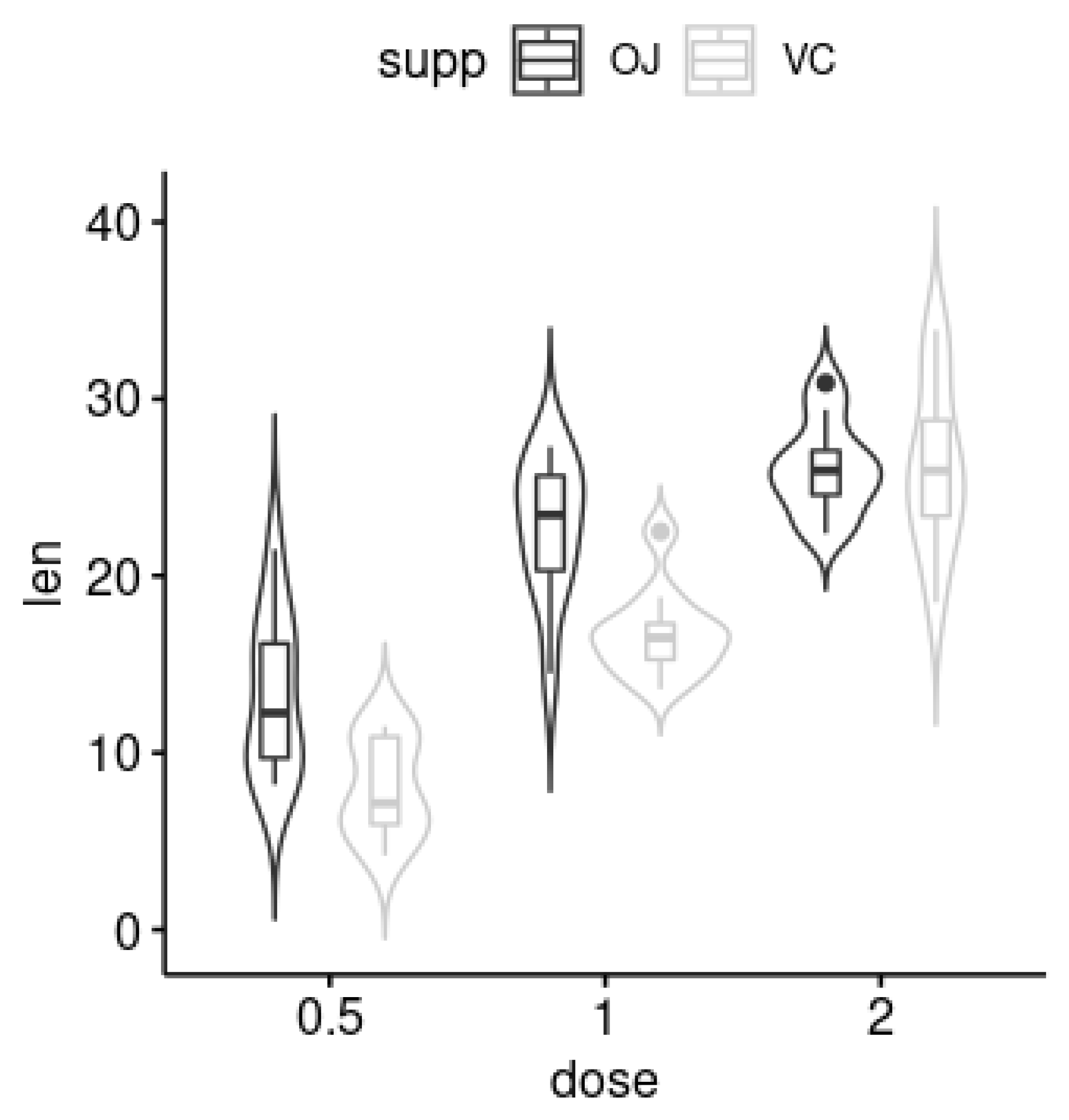
In many practical situations, involving high-dimensional or structured data sets, few explanatory variables are continuous. Many of them are qualitative variables, counts or dummies; and others, though continuous in nature, are recorded as intervals and can be treated as discrete. Generally, those variables describe classes of interest for the researcher. When the number of categories is close to or even greater than the sample size, this results in sparse data.
For overviews and recent developments to efficiently utilize data information from categorical regressors, see [25,26,27,28,29,30,31,32,33,34,35,36]. Our target is to use the prediction methodology described in Section 2 using expression (15) when the regressors are categorical. Since with categorical variables, the notion of Euclidean distance given in expression (15) is not well established; in order to use the empirical similarity, methodology some adaptation is necessary.
Gayer et al. [14] proposed to encode the categorical regressors into dummies, one for each category of each regressor, and apply the weighted Euclidean distance to evaluate similarity. This approach induces for each dummy variable a different weight, even if they come from the same categorical feature, which we see as not intuitive.
For example, suppose a model with a single categorical explanatory variable x 1 , with three levels, denoted by a, b and c. According to Gayer et al. [14], these categories should be encoded into three dummy variables, I a = I ( x 1 = a ) , I b = I ( x 1 = b ) and I c = I ( x 1 = c ) , where I ( · ) is the indicator function. In this way, the model associates for each one of these dummies the weights ω a , ω b and ω c , respectively. Thus, the weighted Euclidean distance between I a and I b , d ω ( I a , I b ) = ω a + ω b , generally is different from distance d ω between I b and I c , i.e.,  d ω ( I b , I c ) = ω b + ω c . Notice that, in this approach, the weights reflect different relative importance for the levels in the categorical variable x 1 and this does not make sense, once differences within levels of the same variable should not be evaluated differently for unordered categorical regressors. This approach also has the disadvantage of increasing the dimensionality of the design matrix X and may turn the prediction by empirical similarity into an ill-posed problem.
In this work, we propose to measure distance using the categorical regressors without encoding them into dummy variables. For that, we propose the use of the following weighted binary distance metric
d ω ( x i , x j ) = k = 1 m ω k I ( x i k , x j k ) ,
where x i = ( x i 1 , , x i m ) and x j = ( x j 1 , , x j m ) are two observations from m categorical regressors, and 
I ( x i k , x j k ) = 0 , if x i k = x j k , ( match ) , 1 , if x i k x j k , ( mismatch ) .
The weighted binary distance in expression (16) is given by the sum of the weights whose explanatory variables are different. This alternative is equivalent to encode the qualitative variables into dummy variables, but constraining the weights to being the same for all levels of the variable without increasing the dimensionality of the design matrix.
Using the distance expression (16) in the similarity functions given in expression (8), we can use the predictor in expression (15). In this approach, the prediction of the response will be given by the weighted average of y’s, where the values of the response variable that have more identical values in the categorical regressors have a greater weight. Under this framework, the parameter estimator of the vector ω is obtained by maximizing the profile likelihood function given in expression (14) and it is denoted by  ω ^ MLE .
Another estimation procedure can be used to obtain the prediction of our model, y ^ t = y ^ ( x t ) (depending on ω ), for a new data point x t . This estimator can be chosen by minimizing a cost function which we take to be the MSE between the predicted and observed values. Formally, we denote the solution to this problem as
ω ^ LS = min ω R + m i = 1 n y i j i j s ( ω ; x i ) y j 2 .
Next, we call by M 1 the model that deals with categorical regressors as proposed here and by M 2 the model proposed by Gayer et al. [14] which uses dummy variables.

4. Application

We apply the proposed methodology to study the effect of Vitamin C supplement on tooth growth in guinea pigs. For that, we use the ToothGrowth data set [37] available in the R software [38]. We used the R software to implement the estimation methodology of the Models M 1 and M 2 and also to fit the linear regression model. The tooth growth data set contains the length of the odontoblasts (y) in 10 guinea pigs according to two delivery methods ( x 1 )(orange juice (OJ) ( x 1 = 0 ) or ascorbic acid (VC) ( x 1 = 1 )) and three Vitamin C dosage ( x 2 ) levels (0.5 ( x 21 ), 1 ( x 22 ), and 2 ( x 23 ) mg). The data set contains 60 observations.
Figure 1 presents the violin plot [39] for the ToothGrowth data set. According to the plot, there exists a different behavior of the response variable across the categorical regressors. Regardless of the supplementation method, there is a clearly observable trend of increased response with increasing dosage levels. Although there is a slight advantage in OJ being more effective than VC for obtaining greater response values, there is no significant statistical difference between supplementation methods, regardless of dose size.
Now, we fit the response using Models M 1 and M 2 discussed in Section 3. For Model M 1 , we associate the weights ω 1 and ω 2 corresponding to dosage level and supplement method, respectively. Since the variable dosage level is ordinal and the variable supplement method has only two values, we used both binary and Euclidean distances to measure similarity in Model M 1 . On the other hand, in Model M 2 , the weights ω 1 , ω 2 , ω 3 and ω 4 correspond to the dummy variables associated with Vitamin C—dose 0.5 mg, Vitamin C—dose 1.0 mg, Vitamin C—dose 2.0 mg and supplement method, respectively.
For comparative effect, we also fit the following linear regression model
y = β 0 + β 1 x 1 + β 2 x 22 + β 3 x 23 ,
where β = ( β 0 , β 1 , β 2 , β 3 ) is the vector of coefficients and the variables x 1 , x 22 and x 23 have been previously defined.
We compared the obtained parameters’ estimates in two scenarios. In Scenario 1, we use the complete database to estimate the parameters and then, with these estimates, we obtain the predictions for the whole database. On the other hand, in Scenario 2, we divided the database into a training database (corresponding to 70% of randomly chosen observations in the database) and a test database (corresponding to the remaining observations). The training database was used to estimate the parameters which were used to predict the response in the test database. Predictions were evaluated by MSE values.
The estimated parameters of Model M 1 using four different methods can be seen in Table 1. The methods differ in the estimation procedure LS or MLE and in the similarity function used FR or EX. Since the weight ω 2 corresponds to the Type of Supplement variable which contains only two possible values, the distance measures match and, consequently, the estimates obtained for ω 2 do not vary much with the choice of distance metric. On the other hand, the estimates of the weight ω 1 , which corresponds to the Vitamin C Dose variable, are greater when the Euclidean distance is used. In both scenarios, for both distance measures and estimation methods, we observed that the largest value of the estimated parameters corresponds to the weight ω 1 , which means that the Vitamin C Dose variable is the most important to predict the tooth growth length of guinea pigs. Moreover, it can be observed that the parameter estimates for the exponential similarity function are less influenced by the estimation method than those for the fractionary similarity function, but are more influenced to changes in the distance metric used.
In Table 2, we present the parameters’ estimates of Model M 2 using the same four methods of the previous analysis. In both scenarios, regardless of the estimation method, the estimates of the weight ω 2 are equal to zero. This result implies that Vitamin C Dose 1.0 milligram variable does not affect the estimation of the tooth length in guinea pigs. The largest estimated weight corresponds to the 0.5 milligrams Vitamin C Dose, followed by the estimated weight corresponding to the 2.0 milligrams Vitamin C Dose and the lowest corresponds to the Type of Supplement variable. Again, the Vitamin C dose is the most influential variable on the prediction of the tooth growth length of guinea pigs. However, note that the interpretation of the results of Model M 2 is harder since the lowest dose showed the highest influence and the intermediate value showed no influence at all—even though, according to the violin plot displayed in Figure 1, this is not the observable trend. Finally, it was also observed that parameters’ estimates for the exponential similarity function are more robust to changes in the estimation method than those for the fractionary similarity function.
The estimates of the parameters of the linear regression model given by Equation (19) can be seen in Table 3. Considering a 1% significance level, all explanatory variables are significant and help to explain the response variable. We highlight that the weight corresponding to the supplement method has different signs depending on the scenario considered. This suggests that the method of empirical similarity is more robust to model this database.
In Table 4, we present the MSE values, for both Models M 1 and M 2 and also for the regression model. In general terms, the MSE values do not vary with the empirical similarity method used. However, in general, LS results are better than those obtained by MLE. In comparison with results from the regression model, it can be seen that regression performed better than the empirical similarity approach in Scenario 1, but in Scenario 2 with LS estimates, empirical similarity obtained the best results. This suggests that regression may be overfitting the training data set.

5. Conclusions and Future Work

We proposed a new similarity model to address the case of categorical explanatory variables ( M 1  model), in which the explanatory variables are considered in its original form without having to code them into dummy variables. This implies that all possible levels of the categorical explanatory variable have the same weight. Therefore, Model M 1 has an advantage of being more parsimonious than that proposed by Gayer et al. [14] ( M 2 model).
We performed an application using the ToothGrowth data set, which contains data about tooth length of guinea pigs feed with Vitamin C with three different dosage levels and two different supplementary methods. We compared both similarity models with the linear regression model under two scenarios: one considering the full database and another randomly splitting the database into training and test subsets. In both scenarios and considering all similarity models, we obtained that the estimates of the weights that accompany the Vitamin C Dose variable are larger than the estimates obtained for the weights of the Type of Supplement variable, implying that this variable is more influential to the prediction of the tooth length in guinea pigs. It was also observed that the relative importance of the Vitamin C Dose variable is higher when the Euclidean distance is used in the M 1 model. Moreover, it was also observed that parameters’ estimates for the exponential similarity function are less influenced by changes of the estimation method than those of the fractionary similarity function, but are more influenced to changes in the distance metric used.
The application also highlights that the interpretation of Model M 2 is harder since, although the lowest dosage of Vitamin C has the highest associated weight, the intermediary dosage showed no influence at all in the response variable, contradicting the increasing observable trend displayed in the violin plot of Figure 1. In what regards the regression model, it is also observed that the sign of the parameter estimate associated with the Type of Supplement variable has changed in the two scenarios analyzed, which suggests that empirical similarity models are more robust to model the ToothGrowth data set.
Through an MSE analysis, we observed that empirical similarity predictions with LS estimates are the best ones for the test data set. On the other hand, regression obtained the best results for the training data set, which suggests that it may be overfitting the training data. As pointed out by an anonymous referee, a penalty item is commonly inserted into the error function as a regularization method when fitting a regression model to data, in order to prevent overfitting [40,41,42]. We do not added such a penalty in our analysis so that a fairer comparison between the methods can be made given that regularization methods have not been proposed yet in the empirical similarity methodology. Having said that, we do agree that the proposal of regularization methods in this methodology is an interesting problem to be handled in a future work. Moreover, in all works in the empirical similarity literature, it is assumed that the error has a fixed variance. In future works, we intend to expand the model to capture heteroscedastic data.

Author Contributions

Conceptualization, L.C.R. and R.O.; Data curation, J.D.S. and R.O.; Formal analysis, J.D.S.; Funding acquisition, L.C.R. and R.O.; Investigation, J.D.S.; Methodology, J.D.S., L.C.R. and R.O.; Project administration, L.C.R. and R.O.; Resources, L.C.R. and R.O.; Software, J.D.S. and R.O.; Supervision, L.C.R. and R.O.; Validation, L.C.R. and R.O.; Visualization, R.O.; Writing—original draft, J.D.S., L.C.R. and R.O.; Writing—review and editing, L.C.R. and R.O.

Funding

This study was financed in part by the Coordenação de Aperfeiçoamento de Pessoal de Nível Superior-Brasil (CAPES)-Finance Code 001. This work was also supported in part by Conselho Nacional de Desenvolvimento Científico e Tecnológico (CNPq) grant number 307556/2017-4 and Fundação de Amparo à Ciência e Tecnologia de Pernambuco (FACEPE) grant number IBPG-0086-1.02/13.

Acknowledgments

The authors thank the editor and anonymous referees for comments and suggestions.

Conflicts of Interest

The authors declare no conflict of interest.

References

  1. Fix, E.; Hodges, J.L. Discriminatory Analysis. Nonparametric Discrimination: Consistency Properties; Technical Report 4; Project Number 21-49-004; USAF School of Aviation Medicine: Randolph Field, TX, USA, 1951. [Google Scholar]
  2. Fix, E.; Hodges, J.L. Discriminatory Analysis: Samall Sample Performance; Technical Report 21-49-004; USAF School of Aviation Medicine: Randolph Field, TX, USA, 1952. [Google Scholar]
  3. Cover, T.M.; Hart, P.E. Nearest Neighbor Pattern Classification. IEEE Trans. Inf. Theory 1967, 13, 21–27. [Google Scholar] [CrossRef]
  4. Devroye, L.; Gyorfy, L.; Lugosi, G. A probabilistic Theory of Pattern Recognition; Springer: New York, NY, USA, 1996. [Google Scholar]
  5. Akaike, H. An approximation to the density function. Ann. Inst. Stat. Math. 1954, 6, 127–132. [Google Scholar] [CrossRef]
  6. Rosenblatt, M. Remarks on some Nonparametric Estimates of a Density Function. Ann. Math. Stat. 1956, 27, 832–837. [Google Scholar] [CrossRef]
  7. Parzen, E. On the Estimation of a Probability Density Function and the Mode. Ann. Math. Stat. 1962, 33, 1065–1076. [Google Scholar] [CrossRef]
  8. Silverman, B.W. Density Estimation for Statistics and Data Analysis; Chapman & Hall: London, UK, 1986. [Google Scholar]
  9. Scott, D.W. Multivariate Density Estimation: Theory, Practice and Visualization; Wiley: New York, NY, USA, 1992. [Google Scholar]
  10. Gilboa, I.; Lieberman, O.; David, S. Empirical Similarity. Rev. Econ. Stat. 2006, 88, 433–444. [Google Scholar] [CrossRef]
  11. Gilboa, I.; Schmeidler, D. Case-based decision theory. Q. J. Econ. 1995, 110, 605–639. [Google Scholar] [CrossRef]
  12. Gilboa, I.; Schmeidler, D. A Theory of Case-Based Decisions; Cambridge University Press: Cambridge, UK, 2001. [Google Scholar]
  13. Gilboa, I.; Schmeidler, D. Inductive inference: An axiomatic approach. Econometrica 2003, 71, 1–26. [Google Scholar] [CrossRef]
  14. Gayer, G.; Gilboa, I.; Lieberman, O. Rule-Based and Case-Based Reasoning in Housing Prices. BE J. Theor. Econ. 2007, 7. [Google Scholar] [CrossRef] [Green Version]
  15. Gilboa, I.; Lieberman, O.; Schmeidler, D. A similarity-based approach to prediction. J. Econ. 2011, 162, 124–131. [Google Scholar] [CrossRef] [Green Version]
  16. Lieberman, O. Asymptotic Theory for Empirical Similarity Models. Econ. Theory 2010, 4, 1032–1059. [Google Scholar] [CrossRef]
  17. Lieberman, O. A Similarity-Based Approach to Time-Varying Coefficient Non-Stationary Autoregression. J. Time Ser. Anal. 2012, 33, 484–502. [Google Scholar] [CrossRef]
  18. Davison, A.C. Statistical Models; Cambridge University Press: Cambridge, UK, 2003. [Google Scholar]
  19. Wassermann, L. All of Nonparametric Statistics; Springer: New York, NY, USA, 2006. [Google Scholar]
  20. Billot, A.; Gilboa, I.; Samet, D.; Schmeidler, D. Probabilities as similarity-weighted frequencies. Econometrica 2005, 73, 1125–1136. [Google Scholar] [CrossRef]
  21. Billot, A.; Gilboa, I.; Schmeidler, D. Axiomatization of an exponential similarity function. Math. Soc. Sci. 2008, 55, 107–115. [Google Scholar] [CrossRef] [Green Version]
  22. Gilboa, I.; Lieberman, O.; Schmeidler, D. On the definition of objective probabilities by empirical similarity. Synthese 2010, 172, 79–95. [Google Scholar] [CrossRef]
  23. Lieberman, O.; Phillips, P.C. Norming Rates and Limit Theory for Some Time-Varying Coefficient Autoregressions. J. Time Ser. Anal. 2014, 35, 592–623. [Google Scholar] [CrossRef]
  24. Hamid, A.; Heiden, M. Forecasting volatility with empirical similarity and Google Trends. J. Econ. Behav. Organ. 2015, 117, 62–81. [Google Scholar] [CrossRef]
  25. Gayer, G.; Lieberman, O.; Yaffe, O. Similarity-based model for ordered categorical data. Econ. Rev. 2019, 38, 263–278. [Google Scholar] [CrossRef]
  26. Aitchison, J.; Aitken, C.G. Multivariate binary discrimination by the kernel method. Biometrika 1976, 63, 413–420. [Google Scholar] [CrossRef]
  27. Delgado, M.A.; Mora, J. Nonparametric and semiparametric estimation with discrete regressors. Econom. J. Econom. Soc. 1995, 63, 1477–1484. [Google Scholar] [CrossRef]
  28. Chen, S.X.; Tang, C.Y. Nonparametric regression with discrete covariate and missing values. Stat. Its Interface 2011, 4, 463–474. [Google Scholar] [CrossRef] [Green Version]
  29. Nie, Z.; Racine, J.S. The crs Package: Nonparametric Regression Splines for Continuous and Categorical Predictors. R J. 2012, 4, 48–56. [Google Scholar] [CrossRef]
  30. Ma, S.; Racine, J.S. Additive regression splines with irrelevant categorical and continuous regressors. Stat. Sin. 2013, 23, 515–541. [Google Scholar]
  31. Chu, C.Y.; Henderson, D.J.; Parmeter, C.F. Plug-in bandwidth selection for kernel density estimation with discrete data. Econometrics 2015, 3, 199–214. [Google Scholar] [CrossRef]
  32. Guo, C.; Berkhahn, F. Entity embeddings of categorical variables. arXiv 2016, arXiv:1604.06737. [Google Scholar]
  33. Racine, J.; Li, Q. Nonparametric estimation of regression functions with both categorical and continuous data. J. Econ. 2004, 119, 99–130. [Google Scholar] [CrossRef] [Green Version]
  34. Li, Q.; Racine, J. Nonparametric estimation of distributions with categorical and continuous data. J. Multivar. Anal. 2003, 86, 266–292. [Google Scholar] [CrossRef] [Green Version]
  35. Li, Q.; Racine, J.S.; Wooldridge, J.M. Estimating average treatment effects with continuous and discrete covariates: The case of Swan-Ganz catheterization. Am. Econ. Rev. 2008, 98, 357–362. [Google Scholar] [CrossRef]
  36. Farnè, M.; Vouldis, A.T. A Methodology for Automatised Outlier Detection in High-Dimensional Datasets: An Application to Euro Area Banks’ Supervisory Data; Working Paper Series; European Central Bank: Frankfurt, Germany, 2018. [Google Scholar]
  37. Crampton, E.W. The growth of the odontoblasts of the incisor tooth as a criterion of the vitamin C intake of the guinea pig. J. Nutr. 1947, 33, 491–504. [Google Scholar] [CrossRef]
  38. R Core Team. R: A Language and Environment for Statistical Computing; R Foundation for Statistical Computing: Vienna, Austria, 2018. [Google Scholar]
  39. Hintze, J.; Nelson, R.D. Violin Plots: A Box Plot-Density Trace Synergism. Am. Stat. 1998, 52, 181–184. [Google Scholar]
  40. Tutz, G.; Gertheiss, J. Regularized regression for categorical data. Stat. Model. 2016, 16, 161–200. [Google Scholar] [CrossRef]
  41. Chiquet, J.; Grandvalet, Y.; Rigaill, G. On coding effects in regularized categorical regression. Stat. Model. 2016, 16, 228–237. [Google Scholar] [CrossRef]
  42. Tibshirani, R.; Wainwright, M.; Hastie, T. Statistical Learning with Sparsity: The Lasso and Generalizations; Chapman and Hall/CRC: Boca Raton, FL, USA, 2015. [Google Scholar]
Figure 1. Violin plots of odontoblasts’ length by dose across the delivery method.
Make 01 00038 g001
Table 1. Parameter estimates of Model M 1 .
Binary Dist.Euclidean Dist.
Method ω ^ 1 ω ^ 2 ω ^ 1 ω ^ 2
Scenario 1LS FR499.5914.721049.2014.79
LS EX5.282.7417.092.71
MLE FR38.324.2352.334.66
MLE EX3.181.626.371.55
Scenario 2LS FR113.176.67170.426.94
LS EX3.911.9612.061.94
MLE FR23.843.5732.754.00
MLE EX2.701.484.821.38
Table 2. Parameter estimates of Model M 2 .
Method ω ^ 1 ω ^ 2 ω ^ 3 ω ^ 4
Scenario 1LS FR719.350.00105.8815.42
LS EX3.790.003.562.84
MLE FR30.600.0020.684.45
MLE EX2.350.002.241.68
Scenario 2LS FR86.650.0046.556.94
LS EX2.720.002.531.97
MLE FR25.200.007.624.04
MLE EX2.120.001.581.57
Table 3. Linear regression model.
Estimates.e.p-Value
Scenario 1Intercept12.460.99 < 0.01
Supp. VC−3.700.99<0.01
Dose 1.0 mg9.131.21<0.01
Dose 2.0 mg15.501.21<0.01
Scenario 2Intercept9.281.16<0.01
Supp. VC3.761.20<0.01
Dose 1.0 mg8.521.49<0.01
Dose 2.0 mg14.261.47<0.01
Table 4. MSE of predictions of the tooth length in guinea pigs.
LSMLE
Method y ^ FR y ^ EX y ^ FR y ^ EX
Scenario 1 M 1 (binary)14.5414.5415.3915.36
M 1 (Euclidean)14.5514.5415.4516.40
M 2 14.5414.5115.3515.19
Regression13.67---
Scenario 2 M 1 (binary)14.5114.8818.0018.41
M 1 (Euclidean)14.4014.0417.5418.55
M 2 14.6915.2718.1918.15
Regression15.31---

