1. Introduction
Automatic speaker recognition is a challenging task as speakers may have different accents, pronunciations, styles, word rates, and emotional states. Furthermore, the presence of environmental noise makes the task even more challenging. Development of a functional speaker recognition architecture has paved the way for many real-world applications such as speech forensics, robotics, and home control systems [
1]. In several areas, recorded voice has been traditionally used to collect data through transcription. Healthcare is one such area where the voice is recorded for later reporting. Moving further towards real-world applications in healthcare, researchers have now been focusing on point-of-impact technologies. Statistically, medical first responders making a large number of errors during transfer of care, leading to loss of human lives, is considered as the primary reason for this shift [
2]. It is notable that limited response time, lack of standard technical language/protocol, and the difference in knowledge of equipment among the caretakers, serve as primary sources of these errors. It is expected that the use of a speaker recognition system integrated with an existing Natural Language Processing (NLP) system for voice-activated decision making or
synthetic assistance (SA), might reduce such errors to some extent, and improve the voice-based UI while providing secure access to these systems [
3,
4]. Such systems, involving the use of
synthetic assistants (SA) or voice-activated decision-making, would also require authentication through speaker recognition.
We propose the use of an in-house developed synthetic assistant for such applications to minimize errors by augmenting a medic’s capabilities through assistance in decision-making. A personalized voice assistant with custom-built skills would be a great example of an SA for such applications. However, these commercial off the shelf (COTS) devices and the associated applications are available to the public and may pose security and privacy challenges if access is not limited. One of the ways to limit access can be a high-accuracy real-time speaker recognition system. Motivated by the applications of real-time speaker recognition, we propose a generalized speaker recognition architecture that can be used in near real-time without compromising accuracy. Furthermore, the proposed architecture overcomes the issue of recognizing a single speaker when multiple non-overlapping speakers are present in a noisy environment. The proposed architecture would also make the recognition simpler and allow further integration with other existing NLP systems.
Classification algorithms and feature extraction techniques are integral components of a speaker recognition system. Several algorithms for speaker recognition have been proposed over the years with varying degrees of success. Conventional speaker recognition systems used a Gaussian mixture model (GMM)-based hidden Markov models (HMMs) [
5]. However, it was inefficient for modeling data that lie on or near a non-linear manifold in the data space. To understand this concept, consider an example of modeling the set of points that lie closer to the surface of a sphere. Those points would only require a few parameters using an appropriate model class. On the contrary, it would require a large number of diagonal Gaussians or full-covariance to model them. Later on, with the development of various machine learning (ML) algorithms, the research community shifted its focus to algorithms such as support vector machine (SVM), random forest (RF), Linear Regression, K-Nearest Neighbors, K-means, and most recently, deep neural network (DNN). Among these, we found that SVM, RF, and DNN exhibit the best performance in recent works [
6].
Researchers identified random forest as the best classifier among 179 classifiers considered in their study [
7]. However, another group of researchers claimed that these results lacked a held-out test set and excluded trials with errors [
8]. Furthermore, the statistical tests in [
7] showed that RF did not have higher percentage accuracy than SVM and artificial neural networks (ANNs). Therefore, in our work, we explore SVM, RF, and DNN classifiers to determine which one would be the best for speaker recognition. It is also noteworthy that choosing the correct classifier does not mean that the speaker recognition problem is solved and care should be taken to ensure that an optimal set of features are being extracted from the speech sample under consideration. Although features such as pitch, zero-crossing rate (ZCR), short-time energy (STE), spectral centroid (SC), spectral roll-off (SR), and spectral flux (SF) have been previously used in speaker recognition, they are more suitable for background noise detection [
9,
10,
11]. Similarly, Mel frequency cepstral coefficients (MFCC) have also been used in speaker recognition, but they tend to give unreliable results in noisy environments [
12].
This paper contributes to the area of speech processing by proposing a voice authentication based access to an NLP system. Voice authentication is accomplished by developing a generic and robust speaker recognition architecture that could be integrated with an existing cloud-based NLP. The paper also gives insights into the essential features of speech signals that are vital to training popular ML algorithms for speaker recognition. Insight into features was achieved through a detailed performance analysis of different ML algorithms using the standard ELSDSR and in-house generated dataset. The proposed novel architecture uses GF, CNN, and statistical parameters separately for feature extraction. Also, we briefly discuss ML algorithm-based classifiers such as RF, SVM, and DNN and present results related to their behavior when used with different datasets. Finally, we compare our architecture performance to the standard AlexNet architecture [
13].
The rest of the paper is organized into six sections.
Section 2 discusses the most relevant related work in speaker recognition.
Section 3 presents our proposed high-speed pipelined architecture.
Section 4 details the pre-processing and feature extraction modules of the proposed architecture.
Section 5 presents a detailed discussion on ML-based algorithms that have been used in speaker recognition applications.
Section 6 presents our experimental results and related discussion. Finally, we conclude the paper with comments on possible future work directions along with limitations.
2. Related Work
In this section, we discuss existing architectures including the authentication process, and techniques that have been used for speaker recognition. After a detailed literature survey, we found that very few architectures for speaker recognition or related areas have been proposed to date. We found that it was difficult to ascertain if one of the most recent attempts to address multilingual speech recognition architecture can be used for speaker recognition [
14]. On top of that, the authors also did not mention if this architecture is compatible with cloud-based NLP applications. On a positive note, this architecture is well-defined and is expected to be useful for real-time applications. Other popular architectures in literature are simple in design and use old classification algorithms and feature extraction techniques [
1,
15,
16]. These architectures also lack real-time applicability.
One of the most recently proposed (2019) fully supervised speaker diarization framework [
17] proposes an “
online system with offline quality.” This work proposes the use of unbounded interleaved-state RNN (UIS-RNN) which is a trainable model and outperforms the spectral offline clustering algorithm on the NIST SRE 2000 CALLHOME benchmark [
18]. Another recent work proposes a speaker verification framework using CNN with a focus on demonstrating the use of effective pair selection for verification [
19]. This work primarily leverages the protocol proposed by authors of
Voxceleb database [
20]. In related authors published part 2 of the work where
Voxceleb data is used in speaker recognition using CNN models. The paper examines the depth of network with performance and results conclude substantial performance improvement with performance improves with greater network depth [
21]. Another Deep CNN and LSTMs were used for ASR acoustic modeling [
22] with accuracies ranging between 69–83% for various scenarios, using the TIMIT database [
23]. A 2018 work also proposes a text-independent ASR using LSTM which creates match and non-match pairs for ASR through learning the speaker as well as the background sound [
24]. Similar to [
18], this model uses overlaps in signal windows during feature extraction to capture temporal variations and suggests that LSTM fails to capture long dependencies in speaker characteristics. In another CNN and Gaussian mixture model (GMM) speaker recognition model authors used spectrograms to recognize the speaker to recognize short utterances and results presented are promising [
25]. The recent LSTM based works further conclude that LSTM has not been successful in capturing long dependencies among speaker characteristics while trying to capture temporal speech variation [
18,
26].
Few researchers have also focused on authenticating along with recognizing an individual’s voice by comparing the collected voice template for training and testing [
27,
28]. However, architecture performance was not reported for noisy or real-time environments. Similarly, another work focused on building a secure real-time android-based speaker recognition system to identify the technician’s voice in the laboratory [
29]. In this work, the authors state that the authentication process is complicated in noisy environments. Moreover, the authors did not report any performance-related results of the proposed system. Similarly, different classification and feature extraction techniques have been used in automatic speech recognition (ASR), which can be used for speaker recognition as well with some improvements. DNN and CNN have both been successfully applied to ASR with cepstral coefficient features as input to these networks. These researchers found CNN to perform better than DNN and both of these to perform better than GMM/HMM [
30,
31]. However, some researchers have just applied the CNN model for both feature extraction and classification [
32]; and reported the error rate reduction compared to DNN. Researchers have also used CNN as a feature extractor and linear classifiers as a classifier and reported better performance compared to the CNN alone as a feature extractor and classifier [
33].
Similarly, another work employed Gabor filter (GF)-based features for ASR [
34]. The generated features were classified using different classifiers. This work claims that the GF-based feature extraction method gave better recognition than those of MFCC, perceptual linear predictive (PLP) and LPC. In the past, features generated from GF have been used as inputs to DNN to generate Gabor-DNN features and to CNN for improved speech recognition [
12,
35,
36]. One such research incorporated GF into convolution filter kernels where a variety of Gabor features served as the feature maps of the convolution layer [
12]. The authors achieved a better result compared to when Gabor features were used without CNN. It was then concluded that the CNN or DNN features alone are not enough and better speaker recognition is achieved when Gabor features are also incorporated. Similarly, in another recent work, the authors reported a method where specific weight kernels of a CNN are replaced with GF to reduce the training complexity of CNN [
37]. This work claims that a better performance in terms of time and energy was achieved compared to CNN because the convolutional layers use the GF as fixed weight kernels that extract intrinsic features with regular trainable weight kernels. This implementation used the MNIST, FaceDet and TICH datasets. These findings motivated our research towards the development of a novel architecture design that uses GF, CNN, and statistical parameters separately for feature extraction.
3. High Speed Pipelined Architecture
The proposed high-speed pipelined architecture depicted in
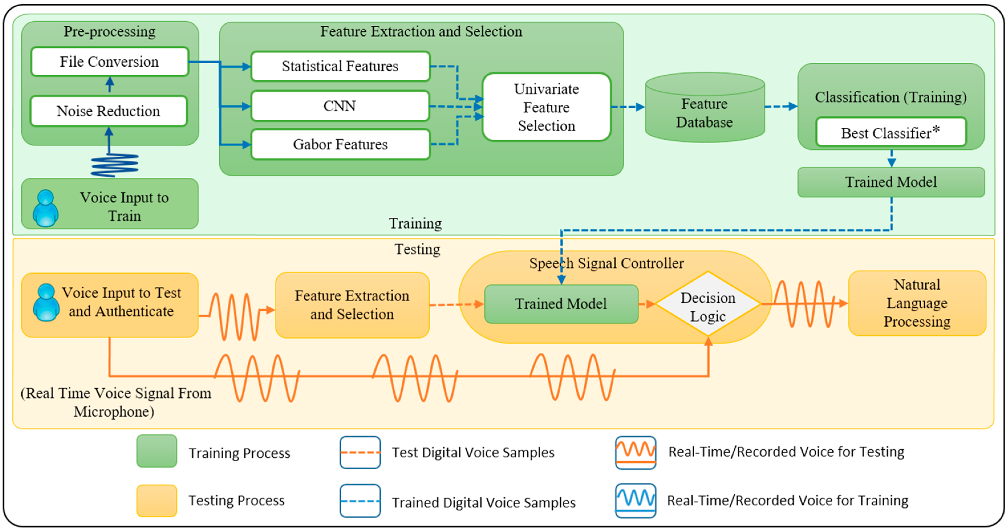
Figure 1 comprises the following blocks: pre-processing, feature extraction, feature selection, classification, trained model, and the speech signal controller block (SSCB). This architecture was designed with the aim to make it simple, highly accurate, and reliable in a noisy environment with the capability to recognize non-overlapping multiple speakers. It was also considered necessary for the architecture to be compatible with cloud-based applications such as popular NLP systems. The proposed architecture consists of different modules, and each of them has been discussed in detail in the paper. In the following paragraphs, we present details of the operation of the proposed architecture.
Suppose that there are six individuals - A, B, C, D, E, and F, all of whom are talking and trying to access the NLP. Let us also assume that the system has been trained to only detect the user B. The proposed high-speed pipelined architecture will recognize only B as the correct person and send B’s voice to the NLP system. Later, if the system designer decides to give access to C as well, then the feature database will be updated with the features of C’s voice. Next, an updated trained model will be generated based on the new feature database. Now, using the generated trained model as a reference, SSCB will start accepting and transferring the voice of both users B and C to the NLP system.
As shown in
Figure 1, after the acquisition of a real-time speech signal, the pre-processing block performs noise reduction and file conversion to a suitable format. Next, the feature extraction block extracts features from the provided voice sample including statistical features, Gabor features, and CNN-generated features. After that, the feature selection block uses the univariate feature selection technique that selects the best features from the extracted features based on univariate statistical test and sends them to the feature database.
Using the feature database the classification block employs the best ML algorithm and builds a trained model. The proposed architecture uses several ML algorithms, and for each new user, the SSCB will train them and then select one of the algorithm mentioned above based on the highest accuracy. A separate set of experiments were performed (discussed in
Section 6) to study the best classifier where we compared three ML-based classifiers. These ML-based classifiers include SVM, RF, and DNN. The classifier that gave the result with the highest accuracy within a given time was selected as the best classifier to build a trained model. The trained model is then stored in the SSCB for comparison with the real-time test voice signals.
Finally, the SSCB uses the extracted features from the test speech signal, tests it against the trained model and makes the decision of sending the captured real-time speech signal to the NLP system. This block will reject the captured real-time speech signal if it fails to pass the test against the trained model. In essence, the SSCB acts as a final switch in the proposed architecture and recognizes individuals for whom the classification algorithm has already been trained while samples from new unauthorized users will not be recognized. This systematic approach in our proposed architecture operation results in a robust speaker recognition process. In the subsequent sections, we will discuss the submodules of the proposed architecture in more detail.
4. Preprocessing and Feature Extraction
The preprocessing consists of a series of steps including noise separation and file conversion. First, the Additive White Gaussian Noise (AWGN) corrupting the input audio signal is filtered. We used the Recursive Least Squares (RLS) adaptive filtering method for the noise cancellation [
38]. Since the feature extraction technique for our proposed architecture requires the input to be an image [
33], we represent the received audio file as a spectrogram. Spectrograms are 2D images representing sequences of spectra with time and frequency along each axis with brightness or color intensity representing the strength of a frequency component at each timeframe [
39]. A spectrogram is limited in the sense that it can only show one channel at a time because of its 2D nature. To overcome this limitation, we averaged two channels of the received audio signal before converting it to a spectrogram.
Extraction of a set of features from the voice signal is an essential step for the classification of speakers. We extracted features using statistical parameters, GF, and CNN from the spectrograms generated using the raw voice signals. The feature selection on each of these parameter set was performed to obtain the best feature set.
To test the proposed architecture in the stages of preprocessing and feature extraction, we used two data sets. As presented in
Table 1, dataset 1 is a standardized dataset called ELSDSR [
40] that generally used speaker recognition. Dataset 2 is an in-house developed dataset with more realistic conditions and background noises than any scandalized dataset collected in a controlled environment. One of the reasons to come up with an in-house dataset is that Nationality plays a vital role in the accent of different speakers. The aim of the new data (i.e., dataset 2) was to be more compatible with newer NLP systems that can recognize various English accents. If the non-native speaking user decides to get access to the NLP system, then our proposed architecture should be able to provide proper authentication to those new users. The primary objective of our architecture was to authenticate speaker and provide secure access to NLP systems. Typically, speakers from any nation could use existing NLP systems. Therefore, with diverse nationality, we aimed to check the robustness and accuracy of our architecture for various accents. There are several large data sets available for researchers of voice recognition and authentication used by previous publications example
Voxceleb database [
20]. The rationale for not using large data sets such as Voxceleb, or Harvard-Haskins is our model targeting applications of sensitive environments. Our tested architecture should tell who specifically in the system is instead of who is not in the system. In the real world, application the users going to submit only one are two user voice sample for authentication in their personal assisting devices, so in most of the cases, our architecture has to work with a very sparse and small data set. The main aim of proposing this architecture was to provide secure user access to an existing NLP system. Based on our application domain, we wanted a limited dataset and therefore, generated in-house data and looked for similar standard datasets. We found ELSDSR data to be the most appropriate for our application. The following subsections detail the feature selection process and the features that were considered during the selection process.
4.1. Statistical Features
The statistical features hold unique value for each pixel in an image and are considered useful for classification. Furthermore, these features give a good indication of the various image intensity-level distribution properties such as uniformity, smoothness, flatness, and contrast [
41]. The statistical features include mean (M), median (Md), standard deviation (SD), and interquartile range (IQR). An example of k-fold cross-validation of statistical values is extracted and shown in
Table 2.
4.2. Gabor Filter
GF is a transform-based method for extracting the texture information. The advantage of this technique is its degree of invariance to scale, rotate, and translate. A GF is a sinusoid function modulated by a Gaussian and is defined by the following equation [
42].
The input parameter ‘
σ’ represents the standard deviation of the Gaussian function, ‘
λ’ represents the wavelength of harmonic function, ‘
θ’ is the orientation, ‘
γ’ is the spatial aspect ratio with a constant value of 0.5, and ‘
ψ’ represents the phase shift of harmonic function. The spatial frequency bandwidth is constant and is equal to 1. The output value is the weight of the filter at the (
x,
y) location. Here, we used 2D GFs that are equally spaced in orientation (i.e., equal
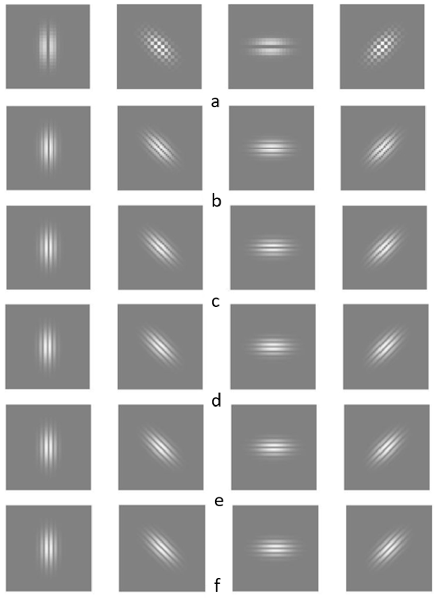
θ) to capture the maximum number of characteristic textural features [
43]. These 24 different GFs were tuned to four orientation values (
θ = 0°, 45°, 90°, and 135°) and six frequencies
(1/λ) (where,
λ = 2.82, 5.65, 11.31, 22.62, 45.25, 90.50) as shown in
Figure 2.
4.3. Convolution Neural Network (CNN)
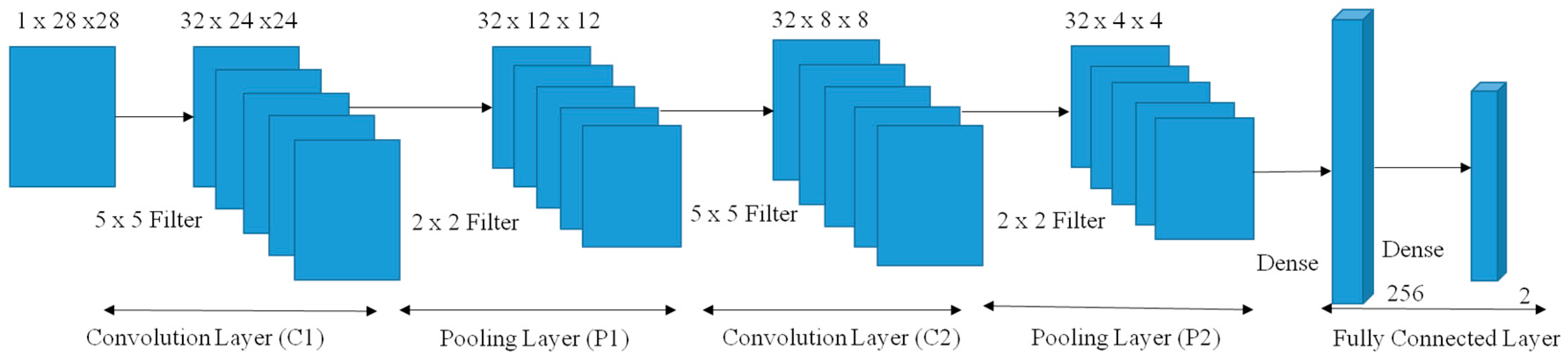
The CNN shown in
Figure 3 is five layered. Namely, two convolution layers, C1 and C2, and two pooling layers, P1 and P2, and an output layer [
44,
45]. The size of the filter used in convolution layers C1 and C2 was 5 × 5 whereas the filter size used in pooling layers P1 and P2 was 2 × 2. The input to the CNN was 28 × 28 grayscale images. The output of C1 and C2 give a feature map of 32 sets for both of them. The outputs of P1 and P2 had the same number of feature map sets as C1 and C2. The output of the CNN was a column vector of dimension 256 × 1 that was used by the SoftMax classifier to classify the input images into one of the two output classes. The last two layers of the CNN classifier, i.e., P2 and the output layer, were fully-connected. The CNN classifier was trained using the back-propagation algorithm in batch mode, and the architecture was implemented using the python packages lasagne and nolearn [
46,
47,
48]. According to the discussion presented in [
46,
47,
48] when the training dataset is spectrographic, a 5 × 5 filter has shown better output with 32 pooling channels and two max-pooling layers. Other models that literature tested include 3 × 3 and 11 × 11 with 16 channels and 64 channels where we retested their models and out test showed no difference in results compared to the cited research works. The dense layer was also used between P2 and the output layer to avoid overfitting. Finally, the set of weights and bias parameters obtained after training the samples were used to extract features from the P2 layer considered as the bottleneck layer.
This CNN model was trained with both standard data (ELSDSR) [
45] and the collected 26 voice samples that were converted to an image.
4.4. Feature Selection
The feature selection technique is found to be helpful before data modeling as it reduces overfitting, improves accuracy and reduces the model complexity. Feature selection further makes the model easier to interpret and reduces training time. In the proposed architecture, to achieve these advantages, we implemented the univariate feature selection technique. This feature selection technique works by selecting the best feature based on univariate statistical tests. In particular, the chi-square test was performed on the samples to obtain the 56 best features from the 286 extracted features. The use of chi-square test was based on its property of selecting the informative features and removing the redundant values. Moreover, it helps reduce large feature sets by selecting the highest scoring feature based on the statistical test. The main objective to use this feature selection technique was to reduce our extracted feature matrix to a smaller size so that the training time is decreased with no loss of accuracy. The results of the experiments performed with the univariate feature selection technique are discussed in
Section 6. Based on the univariate statistical test when
k = 1, one best feature is selected. Similarly, for the value of
k = 2 and
k = 3, two and three best features are selected from four extracted feature.
4.5. Comparative Study
To evaluate the efficacy of the selected feature set, we compared the performance of the proposed framework with a few features or feature sets that have been popularly used in literature such as MFCC, ZCR, Pitch, SC, SR, SF, and STE [
9,
10,
11,
12]. These feature(s) have been widely studied in different application scenarios where primary training dataset was large with sample size 1000 and above. The main purpose of the comparative study was to show how the proposed feature extraction technique performs as compared with popular feature extraction methods when used with standard classifiers. The results of this study are presented and discussed in
Section 6.1. Here is a short description of these popular features:
MFCCs are derived from a cepstral representation of the audio clip, which is the amplitude of the resulting spectrum of the frequency bands that are equally spaced on the
mel scale [
12].
ZCR of a speech signal is the sign change along the signal, i.e., the rate at which the signal changes, and is a good indication of the speech variability [
10].
STE is a good measure of the total energy in a short analysis frame of the voice signal and calculated by windowing of the speech sequence and summation of energy in that short window [
10].
SR is the frequency below which 85% of the total spectrum energy is contained and indicates mean and the variance of the roll-off across timeframes in the texture window [
10,
11].
SC of a speech signal is defined as the center of gravity of the frequency components in the spectrum and is evaluated using Fourier transform [
10,
11]. Perceptually, it indicates the “brightness” of a sound.
SF is the squared difference between the normalized magnitudes of successive spectral distributions and is a good measure of how quickly a local spectral, i.e., the power spectrum of a signal, changes. The mean and the variance of the flux across timeframes are measured through SF [
10,
11].
5. Machine Learning-Based Classifiers
The goal of a classifier is to produce a model, which predicts the target value of the test data given only the test data features. In our architecture, we first compare the results of well-known classifiers from literature and select the classifier with the highest accuracy. We used Python to implement the classifiers. The following sub-sections describe the different classifiers considered in the proposed architecture. Among these classifiers, one with the best classification result was used in the proposed architecture. The comparison of the performance of classifiers has been discussed in
Section 6.2.
5.1. Support Vector Machine
In this work, we treated speaker recognition as a binary classification problem. At each point during the speaker recognition process, we applied the trained classifier to recognize whether the voice is a match or not. We used the radial basis function (RBF) kernel in our experiments due to following reasons: (i) it nonlinearly maps samples into higher dimensional space, (ii) it has less numerical difficulties, and (iii) it has fewer hyper-parameters than the polynomial kernel. Model selection is the process of parameter tuning to achieve high classification accuracy. We used the best pair value for
C and
γ to train the whole training set. The best pair value was found through a grid search method in cross-validation where pairs of values were tested with the training set [
49,
50].
5.2. Random Forest Classifier
RF is the collection of decision trees that uses both bagging and variable selection for tree building, which is built on the bootstrap sample of data [
51]. During the classification, each tree classifies a new object based on attributes, i.e., tree votes for that class. Finally, the classifier chooses the class with the most votes. Two parameters need to be optimized in the RF algorithm: first is the number of variables that are chosen for splitting at each node, denoted by
M, and another is the number of trees to grow or build, denoted by
Ntrees. The selection of
M influences the final error rate. So,
M is usually taken to be a square root of the number of input variables, as was the case in our experiment.
Ntree can be as many as possible as the random forest is fast and there is no overfitting, but for our method, we tried several values using a random function until the prediction error was stabilized.
5.3. Deep Neural Network (DNN) Classifier
DNN is an extension of the ANN with multiple hidden layers between input and output. Extra hidden layers in DNN enable composition of features from lower layers, thus modeling complex data with fewer units as compared to a similarly performing ANN [
5,
52,
53]. In our work, we implemented a DNN with three hidden layers. The hidden units were implemented as Rectified Linear Units (ReLU) such that the input at level
j, which is
xj, is mapped to its respective activation value
yj. The output layer is then configured as a logistic function to obtain an output value between 0 and 1. As a loss function for back propagating gradients in the training stage, we used the cross-entropy function that incorporates the target probability, L2- a regulation parameter that penalizes complex models, and a non-negative hyper-parameter that controls the magnitude of the penalty. The process starts with the initial set of random weight and DNN minimizes the loss function by constantly updating these weights. After computing the loss, a backward pass propagates from the output layer to the previous layers, providing the weight of each parameter with an updated value meant to decrease the loss [
54].
DNN itself performs feature extraction using a stacked sparse encoder or another feature selection method. In our work, we fed DNN classifier with the same features that we fed to the SVM and RF classifier to leverage uniformity in the comparison between these algorithms during feature extraction and selection. Further, we used the asynchronous stochastic gradient descent method for training the DNN. The architecture of the network was 5-layered with 56 input nodes, 3 hidden layers with 50, 100 and 25 nodes, followed by two output nodes. The DNN classifier was implemented using the
TensorFlow library and Python.
Table 3 summarizes the parameters used for DNN in our proposed architecture.
6. Results and Discussion
In this section, we aim to study the perceived performance of the proposed near real-time speaker recognition system. In our algorithm, features were extracted using MATLAB and Python, whereas the classification task was done using Python. Evaluation parameters such as sensitivity, specificity, and accuracy were used to check the performance of ML-based algorithms. Similarly, parameters such as equal error rate (EER), and Detection Error Tradeoff Curve (DETC) were used to evaluate the performance of the speaker recognition architecture. The parameters such as accuracy, specificity, and sensitivity for all the algorithms were calculated using the confusion matrix. The accuracy was calculated using the sum of true positives (TP) and true negatives (TN) divided by total samples. Similarly, sensitivity was calculated using (TP/(TP+FN)), and specificity was calculated using (TN/(TN+FP)) where FP and FN are false positive and false negative respectively.
To validate our architecture, we took standardized data from the English language speech database for speaker recognition (ELSDSR) [
40]. The database contains voice messages from 22 speakers: 12 Males and 10 Females, aged between 24 and 63 from Canada, Denmark, and Iceland. The voice messages were recorded in a .wav format using Pulse Code Modulation. The sampling frequency was 16 KHz, with a bit rate of 16. For training purposes, seven different sentences were collected from each of the 22 speakers. Similarly, for testing purposes, each of the 22 speakers was asked to read two sentences from NOVA Home [
55]. NOVA Home is a web site that contains information about the great pyramid of Egypt. In essence, 154 (7 × 22) utterances were recorded for training, and 44 (2 × 22) utterances were provided for testing.
To test the aforementioned data on our architecture, we divided the training dataset into two different classes, namely known and unknown before training them. A similar process was repeated for testing by classifying them. A comparison of ML-based algorithms based on accuracy, specificity, and sensitivity for standardized data is shown in
Table 4. In the following subsections, we present the results from different submodules of the proposed architecture.
6.1. Evaluation of Extracted Features
A number of features were extracted and studied for real-time speaker recognition; however, our experiments showed that not all of those features were relevant or appropriate. For the experiments, we collected voice samples from 26 speakers, consisting of 15 males and 11 females. Nationality-wise, out of the 26 speakers, 12 were from India, 6 from Nepal, 1 from the Kingdom of Saudi Arabia (KSA), 1 from China and 6 from the USA. The experiments conducted on collected samples from 26 speakers showed that only some features were capable of giving good results.
Apart from the features used in our architecture, we also extracted features such as MFCC, ZCR, pitch, SC, SR, STE, and SF that have been popularly used for speaker recognition as discussed in
Section 4.5 [
9,
10,
11,
12]. All of these extracted features were investigated for speaker recognition using different classifiers to see how they perform when compared with the features used in the proposed framework. A comparison of the accuracy of different classifiers with different features is shown in
Table 5. It can be seen from these results that our proposed feature extraction method provided the best accuracy for all the classifiers considered in the current work.
Similarly, the feature selection technique was performed on each of the extracted features. This technique helped us achieve higher accuracy while reducing training time.
Table 6 reports the improvement in accuracy of ML-based algorithms after the use of the proposed feature selection technique. For this comparison, only a realistic dataset could be used while the dataset 1 (ELSDSR) may not be a reliable source for this specific evaluation since it is collected in a controlled environment without any background noise. Dataset 1 was collected in a controlled environment, but dataset 2 was collected in the real world with all background sounds and uncertainties, which is a requirement for some of the feature extraction methods. Therefore, we only used dataset 2 for this specific purpose.
6.2. Architecture and ML-based Classifier Performance
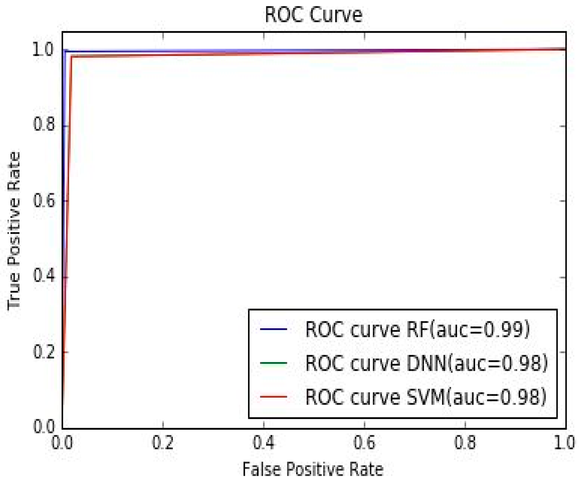
To measure the performance of ML classifiers we used voice samples collected from 26 speakers containing authorized user the need access to NLP. We converted these voice samples to the spectrogram of size 512 × 512 pixels. These spectrograms were further resized to 256 × 256 pixels before extracting features using an array of 24 GFs and statistical parameters. However, in the case of the CNN, for feature extraction, they were resized to 28 × 28 pixels. Next, we used the univariate feature selection technique on the extracted features. After that, the selected features were stored in a database where they were scaled and randomized. Then, these features were separated in the ratio of 4:1 for training and testing. Finally, ML-based algorithms were used for classification to compare the results. The performance was measured using the well-known parameters such as accuracy, sensitivity, and specificity. The specificity parameter, also known as true positive rate, gives the accuracy of framework identifying an authorized user as an authorized user while the sensitivity parameter, also known as true negative rate, gives the accuracy of detecting an unauthorized user as an unauthorized user by each classifier. This analysis is presented in Table 8. In addition, the ROC curve in Figure 5 also shows that the false positive rate, i.e., detection of unauthorized users as authorized users, was very low.
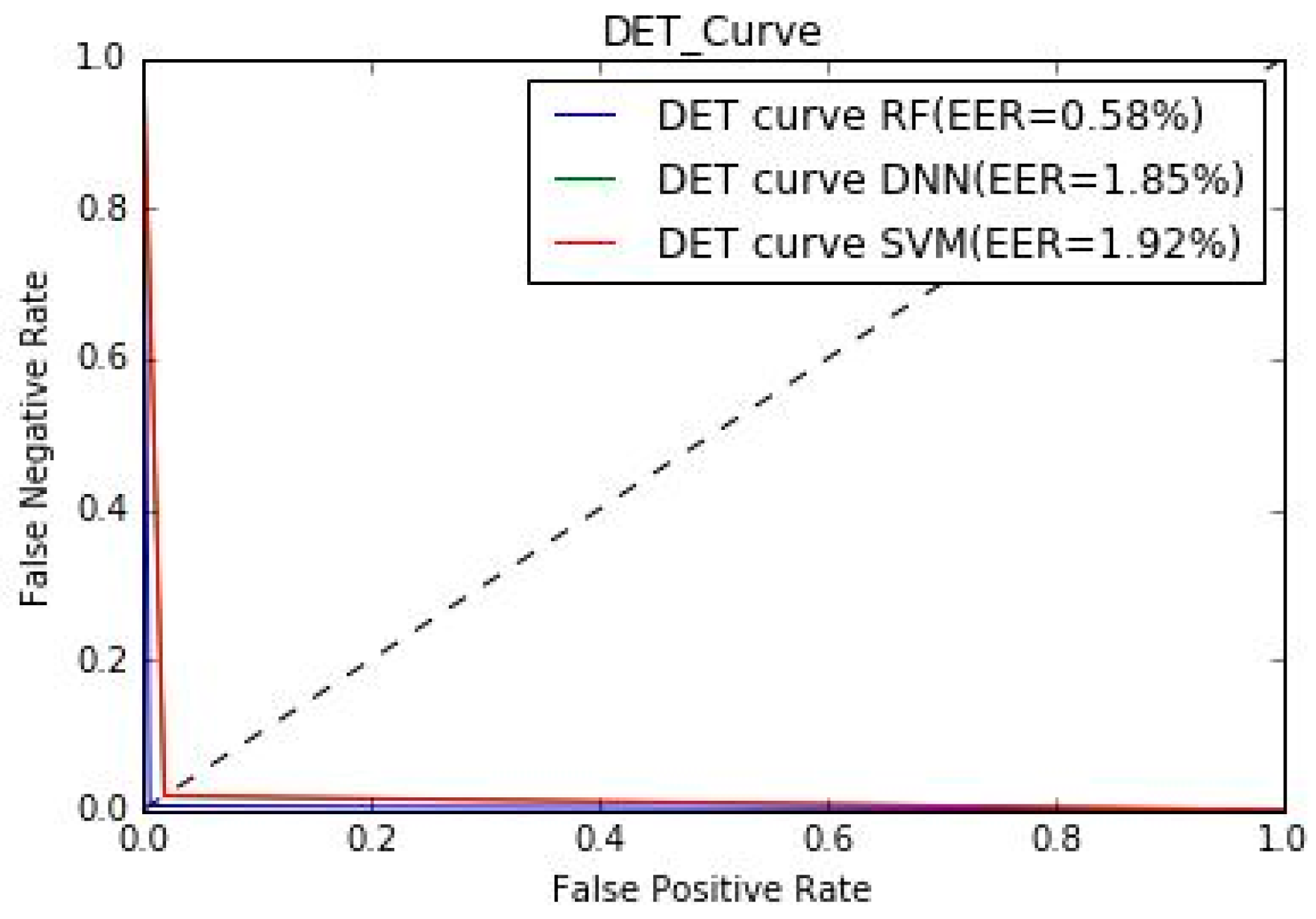
Next, to measure the performance of the speaker-recognition architecture, we used parameters such as equal error rate (EER) and detection error tradeoff curve (DETC) as shown in
Table 7 and
Figure 4, respectively. These parameters are used to show proposed architecture performance in recognized authorized users or rejecting unauthorized user. Moreover, we also compared our architecture with pre-trained AlexNet by providing the same collected samples, as shown in
Table 8. We also found that the %EER were 1.92, 0.58, and 1.85 for SVM, RF, and DNN, respectively. The receiver operating characteristic (ROC) curve, which plots the true acceptance rate versus the false acceptance rate, shown in
Figure 5 demonstrates that the RF algorithm performed better than SVM and DNN for speaker recognition. %EER for the architecture with different classifiers is also shown in
Figure 4 using the DET curve. A DET curve plots the false acceptance rate versus the false rejection rate. This curve moves towards the origin as the system performance improves. With regards to how the performance was measured if the model was trained for A and B, it should be noted that the model was trained on all 26 speaker samples. While evaluating performance, we used the same model that was trained using samples of 26 speakers and passed “new” samples of 5 randomly selected speakers to check if the model can either accept/reject the user as authorized/unauthorized correctly. In other words, the randomly selected speaker could have been of any category, authorized or unauthorized, and was still categorized correctly by the framework.
For standard data, in terms of accuracy, specificity and sensitivity, we obtained 91.66, 93.06 and 90.42 for SVM, 94.87, 97.85 and 92.23 for RF and 93.52, 94.17 and 92.93 for DNN. Similarly, for the collected 26 samples, we obtained 98.07, 98.07 and 98.08 for SVM, 99.41, 99.41 and 99.42 for RF and 98.14, 98.14 and 98.15 for DNN in terms of accuracy, specificity, and sensitivity, respectively. These are listed in
Table 7. Finally, %EER for the proposed architecture with ML algorithms SVM, RF and DNN are 1.92, 0.58 and 1.85, respectively, as shown in
Table 8.
6.3. Real-time Performance of the Architecture
With an aim to study the real-time performance of the proposed architecture with the best classifier, i.e., RF, we randomly chose five speakers out of the samples of 26 speakers from both “known” and “unknown” classes. All these speakers were asked to speak, and then they were authenticated one by one using the proposed framework. From these five speakers, test samples lasting for approximately 5–6 s were taken and tested against the trained model. The average processing time for the proposed architecture, i.e., the time to authenticate after the test sample is received was found to be 0.3456 s, on an average. To perceive any communication real-time bidirectional delays must be of less than 300 ms whereas in our case it is taking little more than that. The time taken for individual samples and the average time of processing has been reported in
Table 9.
With five speakers presented, we were trying to study the average real-time performance of the architecture that did not change much with the complete set of 26 speakers. Using the sample subject size gives us an accurate picture of the average of the overall set of 26 speakers. Initially, we planned to increase the number of speakers if the time taken were not close to each other for different speakers. However, from
Table 9, we can see that those values were quite close to each other, and therefore, we concluded that the time taken to authenticate speakers with only five speakers was a good enough representation of all the speakers in the dataset.
Real-time performance of the architecture enables seamless integration with the cloud-based NLP system without compromising the performance of the NLP system. To examine the integration capabilities of the developed speaker recognition architecture to the cloud-based NLPs, we chose three different NLPs Amazon Alexa [
56], Google Now [
57], and Microsoft Cortana [
58]. All of these services use APIs that provide access to the respective NLP. The interface can be achieved by a far-field or hands-free method of integration where a wake word is used to alert the system. In each case, our developed application will authenticate the speech signal after the wake word. As illustrated in the testing method of our architecture, feature extraction and selection along with a speech signal controller would be a deployment package, which is integrated into the respective APIs. Speech signal controller would be built on a cloud server every time a new speaker’s voice is to be added.
7. Conclusions
In this paper, we presented a novel high-speed pipelined architecture that supports real-time speaker recognition, allowing NLP systems to accept only selected speech signals in near real-time. Most commercially available NLP systems, even after training by a single user, are known to exhibit high false positive rates. The proposed intelligent system attempts to solve this problem by detecting the authorized user with high accuracy. Moreover, we exploit the advantages of GF, CNN, and statistical parameters for feature extraction. Based on our experiments, we found the feature extraction techniques mentioned above and RF to be optimal in speaker recognition for feature extraction and classification, respectively. Our proposed architecture relies primarily on the feature extraction block and classification block for achieving high accuracy. Results of rigorous testing with multiple datasets reveal that RF performed better compared to the other two methods for speaker recognition. While performance decreased in the order of RF-DNN-SVM, the time taken and complexity showed a different trend of decrease in the order of DNN-SVM-RF.
Unlike other approaches, the proposed architecture establishes a mechanism to perform speaker recognition in near real-time. Moreover, we assessed this architecture in terms of both %EER and a DET curve in a collected database consisting of 26 different speakers, with different native languages, and speaking the same language—English. Initially, we hypothesized that we need to train more data points for each accent to be recognized by the model. However, we observed that the model performed equally well regardless of the accent. We also made a comparative analysis of different algorithms based on %EER and a DET curve that is more preferred in the case of the speaker verification system. Finally, the results of the comparison between the proposed and AlexNet architecture show that the proposed architecture is capable of handling and recognizing the voices of multiple individuals without significant impact on accuracy with better performance. This work could be extended in future to identify the voices of multiple individuals talking at the same time, i.e., overlapping voices, possibly using different languages, in real-time (<300ms) and integrated into an NLP system.
Author Contributions
Conceptualization, P.D. (Praveen Damacharla); Data curation, P.D. (Parashar Dhakal); Formal analysis, P.D. (Parashar Dhakal); Funding acquisition, V.D. and A.Y.J.; Investigation, P.D. (Praveen Damacharla); Methodology, P.D. (Parashar Dhakal); Project administration, P.D. (Praveen Damacharla), A.Y.J. and V.D.; Resources, A.Y.J.; Supervision, A.Y.J. and V.D.; Visualization, P.D. (Praveen Damacharla) and A.Y.J.; Writing—original draft, P.D. (Parashar Dhakal); Writing—review & editing, P.D. (Praveen Damacharla), A.Y.J. and V.D.
Funding
This study was funded by Round 1 Project Award “Improving Healthcare Training and Decision Making Through LVC” from the Ohio Federal Research Jobs Commission (OFMJC) through Ohio Federal Research Network (OFRN).
Acknowledgments
This work was partially supported by Department of Electrical Engineering and Computer Science, the University of Toledo and Round 1 Project Award “Improving Healthcare Training and Decision Making Through LVC” from the Ohio Federal Research Jobs Commission (OFMJC) through Ohio Federal Research Network (OFRN). The authors are also thankful to Paul A. Hotmer Family CSTAR (Cyber Security and Teaming Research) lab at the University of Toledo.
Conflicts of Interest
The authors declare no conflict of interest. The funders had no role in the design of the study; in the collection, analyses, or interpretation of data; in the writing of the manuscript, or in the decision to publish the results.
References
- Das, T.; Nahar, K.M. A voice identification system using hidden Markov model. Indian J. Sci. Technol. 2016, 9, 4. [Google Scholar] [CrossRef]
- Makary, M.A.; Daniel, M. Medical error—The third leading cause of death in the US. BMJ 2016, 353. [Google Scholar] [CrossRef] [PubMed]
- Damacharla, P.; Dhakal, P.; Stumbo, S.; Javaid, A.Y.; Ganapathy, S.; Malek, D.A.; Hodge, D.C.; Devabhaktuni, V. Effects of voice-based synthetic assistant on performance of emergency care provider in training. Int. J. Artif. Intell. Educ. 2018. [Google Scholar] [CrossRef]
- Damacharla, P.; Javaid, A.Y.; Gallimore, J.J.; Devabhaktuni, V.K. Common metrics to benchmark human-machine teams (HMT): A review. IEEE Access 2018, 6, 38637–38655. [Google Scholar] [CrossRef]
- Hinton, G.; Deng, L.; Yu, D.; Dahl, G.; Mohamed, A.R.; Jaitly, N.; Senior, A.; Vanhoucke, V.; Nguyen, P.; Kingsbury, B.; et al. Deep neural networks for acoustic modeling in speech recognition: The shared views of four research groups. IEEE Signal. Process. Mag. 2012, 29, 82–97. [Google Scholar] [CrossRef]
- Cutajar, M.; Gatt, E.; Grech, I.; Casha, O.; Micallef, J. Comparative study of automatic speech recognition techniques. IET Signal. Process. 2013, 7, 25–46. [Google Scholar] [CrossRef]
- Fernndez-Delgado, M.; Cernadas, E.; Barro, S.; Amorim, D. Do we need hundreds of classifiers to solve real-world classification problems. J. Mach. Learn. Res. 2014, 15, 3133–3181. [Google Scholar]
- Weinberg, M.; Alipanahi, B.; Frey, B.J. Are random forests truly the best classifiers? J. Mach. Learn. Res. 2016, 17, 3837–3841. [Google Scholar]
- Liu, Z.; Huang, J.; Wang, Y.; Chen, T. Audio feature extraction and analysis for scene classification. J. VLSI Signal. Process. Syst. 1997, 20, 61–79. [Google Scholar] [CrossRef]
- Zahid, S.; Hussain, F.; Rashid, M.; Yousaf, M.H.; Habib, H.A. Optimized audio classification and segmentation algorithm by using ensemble methods. Math. Probl. Eng. 2015, 2015, 209814. [Google Scholar] [CrossRef]
- Lozano, H.; Hernandez, I.; Navas, E.; Gonzalez, F.; Idigoras, I. Household sound identification system for people with hearing disabilities. In Proceedings of the Conference and Workshop on Assistive Technologies for People with Vision and Hearing Impairments, Granada, Spain, 28–31 August 2007. [Google Scholar]
- Chang, S.Y.; Morgan, N. Robust CNN-Based Speech Recognition with Gabor Filter Kernels. In Proceedings of the Fifteenth Annual Conference of the International Speech Communication Association, Singapore, 14–18 September 2014. [Google Scholar]
- Krizhevsky, I.S.; Hinton, G.E. Imagenet classification with deep convolutional neural networks. Adv. Neural Inf. Process. Syst. 2012, 60, 84–90. [Google Scholar] [CrossRef]
- Gonzalez-Dominguez, J.; Eustis, D.; Lopez-Moreno, I.; Senior, A.; Beaufays, F.; Moreno, P.J. A real-time end-to-end multilingual speech recognition architecture. IEEE J. Sel. Top. Signal Process. 2015, 9, 749–759. [Google Scholar] [CrossRef]
- Karpagavalli, S.; Chandra, E. A Review on Automatic speech recognition architecture and approaches. Int. J. Signal. Process. Image Process. Pattern Recognit. 2016, 9, 393–404. [Google Scholar]
- Goyal, S.; Batra, N. Issues and challenges of voice recognition in pervasive environment. Indian J. Sci. Technol. 2017, 10, 30. [Google Scholar] [CrossRef]
- Zhang, A.; Wang, Q.; Zhu, Z.; Paisley, J.; Wang, C. Fully Supervised Speaker Diarization. arXiv preprint 2018, arXiv:1810.04719. Available online: https://arxiv.org/pdf/1810.04719.pdf (accessed on 18 March 2019).
- Zhang, A.; Wang, Q.; Zhu, Z.; Paisley, J.; Wang, C. Fully supervised speaker diarization. In Proceedings of the IEEE International Conference on Acoustics, Speech, and Signal. Processing, Brighton, UK, 12–17 May 2019. [Google Scholar]
- Salehghaffari, H. Speaker Verification using Convolutional Neural Networks. arXiv, 2018; arXiv:1803.05427. [Google Scholar]
- Nagrani, A.; Son, C.J.; Andrew, Z. Voxceleb: A Large-Scale Speaker Identification Dataset. arXiv, 2017; arXiv:1706.08612. [Google Scholar]
- Chung, J.S.; Nagrani, A.; Zisserman, A. VoxCeleb2: Deep Speaker Recognition. Presented at the Interspeech 2018, Hyderabad, India, 6 September 2018; Available online: http://dx.doi.org/10.21437/Interspeech.2018-1929 (accessed on 16 February 2019).
- Xiaoyu, L. Deep Convolutional and LSTM Neural Networks for Acoustic Modelling in Automatic Speech Recognition; Pearson Education Inc.: Hoboken, NJ, USA, 2017; pp. 1–9. [Google Scholar]
- Zue, V.; Seneff, S.; Glass, J. Speech database development at MIT: TIMIT and beyond. Speech Commun. 1990, 9, 351–356. [Google Scholar] [CrossRef]
- Mobiny, A. Text-Independent Speaker Verification Using Long Short-Term Memory Networks. arXiv, 2018; arXiv:1805.00604. [Google Scholar]
- Liu, Z.; Wu, Z.; Li, T.; Li, J.; Shen, C. GMM and CNN hybrid method for short utterance speaker recognition. IEEE Trans. Ind. Inf. 2018, 14, 3244–3252. [Google Scholar] [CrossRef]
- Selvaraj, S.S.P.; Konam, S. Deep Learning for Speaker Recognition. 2017. Available online: https://arxiv.org/ftp/arxiv/papers/1708/1708.05682.pdf (accessed on 18 March 2019).
- Rudrapal, D.; Das, S.; Debbarma, S.; Kar, N.; Debbarma, N. Voice recognition and authentication as a proficient biometric tool and its application in online exam for PH people. Int. J. Comput. Appl. 2012, 39, 12. [Google Scholar]
- Dhakal, P.; Damacharla, P.; Javaid, A.Y.; Devabhaktuni, V. Detection and Identification of Background Sounds to Improvise Voice Interface in Critical Environments. In Proceedings of the 2018 IEEE International Symposium on Signal. Processing and Information Technology (ISSPIT), Louisville, KY, USA, 6–8 December 2018; pp. 78–83. [Google Scholar] [CrossRef]
- Nandish, M.; Balaji, M.C.; Shantala, C.P. An outdoor navigation with voice recognition security application for visually impaired people. Int. J. Eng. Trends Technol. 2014, 10, 500–504. [Google Scholar]
- Sainath, T.N.; Mohamed, A.R.; Kingsbury, B.; Ramabhadran, B. Deep Convolutional Neural Networks for LVCSR. In Proceedings of the IEEE International Conference on acoustics, Speech and Signal Processing, Vancouver, BC, Canada, 26–31 May 2013; Volume 2013, pp. 8614–8618. [Google Scholar]
- Vesely, K.; Karafit, M.; Grzl, F. Convolutive Bottleneck Network Features for LVCSR. In Proceedings of the IEEE Workshop on Automatic Speech Recognition and Understanding (ASRU), Big Island, HI, USA, 11 December 2011; pp. 42–47. [Google Scholar]
- Abdel-Hamid, O.; Mohamed, A.R.; Jiang, H.; Deng, L.; Penn, G.; Yu, D. Convolutional neural networks for speech recognition. IEEE/ACM Trans. Audio Speech Lang. Process. 2014, 22, 1533–1545. [Google Scholar] [CrossRef]
- Poria, S.; Cambria, E.; Gelbukh, A. Deep convolutional neural network textual features and multiple kernel learning for utterance-level multimodal sentiment analysis. EMNLP 2015. [Google Scholar] [CrossRef]
- Missaoui, I.; Zied, L. Gabor Filterbank Features for robust Speech Recognition. In Proceedings of the International Conference on Image and Signal. Processing (ICISP), Cherburg, France, 30 June–2 July 2014; Springer International Publishing: Berlin, Germany, 2014; pp. 665–671. [Google Scholar]
- Martinez, M.C.; Mallidi, S.H.; Meyer, B.T. On the relevance of auditory-based Gabor features for deep learning in robust speech recognition. Comput. Speech Lang. 2017, 45, 21–38. [Google Scholar] [CrossRef] [Green Version]
- Chang, S.Y.; Morgan, N. Informative Spectro-Temporal Bottleneck Features for Noise-Robust Speech Recognition. In Proceedings of the Interspeech 14th Annual Conference of the International Speech Communication Association, Lyon, France, 25–29 August 2013. [Google Scholar]
- Sarwar, S.S.; Panda, P.; Roy, K. Gabor Filter Assisted Energy Efficient Fast Learning Convolutional Neural Networks. In Proceedings of the 2017 IEEE/ACM International Symposium on Low Power Electronics and Design (ISLPED), Taipei, Taiwan, 15 August 2017. [Google Scholar] [CrossRef]
- Mahmoud, W.H.; Zhang, N. Software/Hardware Implementation of an Adaptive Noise Cancellation System. In Proceedings of the 120th ASEE Annual Conference and Exposition, Atlanta, GA, USA, 23–26 June 2013; pp. 23–26. [Google Scholar]
- Wyse, L. Audio Spectrogram Representations for Processing with Convolutional Neural Networks. In Proceedings of the IEEE International Conference on Deep Learning and Music, Anchorage, AK, USA, 18–19 May 2017; pp. 37–41. [Google Scholar]
- Feng, L.; Kai, H.L. A New Database for Speaker Recognition; IMM: Copenhagen, Denmark, 2005. [Google Scholar]
- Malik, F.; Baharudin, B. Quantized Histogram Color Features Analysis for Image Retrieval Based on Median and Laplacian Filters in DCT Domain. In Proceedings of the IEEE International Conference on Innovation Management and Technology Research (ICIMTR), Malacca, Malaysia, 21–22 May 2012; Volume 2012. [Google Scholar]
- Haghighat, M.; Zonouz, S.; Abdel-Mottaleb, M. CloudID: Trustworthy cloud-based and cross-enterprise biometric identification. Exp. Syst. Appl. 2015, 42, 7905–7916. [Google Scholar] [CrossRef]
- Jain, K.; Farrokhnia, F. Unsupervised Texture Segmentation Using Gabor Filters. In Proceedings of the IEEE International Conference on Systems, Man and Cybernetics, Universal City, CA, USA, 4–7 November 1990. [Google Scholar]
- Burkert, P.; Trier, F.; Afzal, M.Z.; Dengel, A.; Liwicki, M. Dexpression: A Deep Convolutional Neural Network for Expression Recognition. arXiv, 2015; arXiv:1509.05371. [Google Scholar]
- Levi, G.; Hassner, T. Age and Gender Classification Using Convolutional Neural Networks. In Proceedings of the IEEE Conference on Computer Vision and Pattern Recognition Workshops (CVPRW), Boston, MA, USA, 7–12 June 2015. [Google Scholar]
- Dieleman, S.; Schlüter, J.; Raffel, C.; Olson, E.; Sønderby, S.K.; Nouri, D.; Maturana, D.; Thoma, M.; Battenberg, E.; Kelly, J.; et al. Lasagne: First release; Zenodo: Geneva, Switzerland, 2015; Volume 3. [Google Scholar]
- Hinton, G.E.; Srivastava, N.; Krizhevsky, A.; Sutskever, I.; Salakhutdinov, R.R. Improving neural networks by preventing co-adaptation of feature detectors. arXiv, 2012; arXiv:1207.0580. [Google Scholar]
- Hijazi, S.; Kumar, R.; Rowen, C. Using Convolutional Neural Networks for Image Recognition; Cadence Design Systems Inc.: San Jose, CA, USA, 2015. [Google Scholar]
- El-Naqa, Y.Y.; Wernick, M.N.; Galatsanos, N.P.; Nishikawa, R.M. A support vector machine approach for detection of microcalcifications. IEEE Trans. Med. Imag. 2002, 21, 1552–1563. [Google Scholar] [CrossRef] [PubMed]
- Hsu, W.; Chang, C.C.; Lin, C.J. A Practical Guide to Support Vector Classification; Technical Report; Department of Computer Science and Information Engineering, National Taiwan University: Taipe, Taiwan, 2003; pp. 1–16. [Google Scholar]
- Liaw, A.; Wiener, M. Classification and Regression by Random Forest; The Newsletter of the R Project; The R Foundation: Vienna, Austria, December 2002; Volume 2/3, pp. 18–22. [Google Scholar]
- Breiman, L.; Friedman, J.; Stone, C.J.; Olshen, R.A. Classification and Regression Trees; CRC press: Boca Raton, FL, USA, 1984. [Google Scholar]
- Tang, Y. Deep learning using linear support vector machines. Presented at the Challenges in Representation Learning Workshop (ICML), Atlanta, GA, USA, 2 June 2013; Available online: https://arxiv.org/pdf/1306.0239.pdf (accessed on 16 February 2019).
- Pedregosa, F.; et al. Scikit-learn: Machine learning in Python. J. Mach. Learn. Res. 2011, 12, 2825–2830. [Google Scholar]
- NOVA, WGBH Science Unit Online; PBS: Washington, DC, USA, 1997; Volume 1, p. 2018.
- Amazon, Alexa. 2018. Available online: Amazon.com (accessed on 18 March 2019).
- Build Natural and Rich Conversational Experiences. 2018. Available online: DialogFlow.com (accessed on 18 March 2019).
- Cortana Is Your Truly Personal Digital Assistant. 2018. Available online: Microsoft.com (accessed on 18 March 2019).
© 2019 by the authors. Licensee MDPI, Basel, Switzerland. This article is an open access article distributed under the terms and conditions of the Creative Commons Attribution (CC BY) license (http://creativecommons.org/licenses/by/4.0/).


