Category Maps Describe Driving Episodes Recorded with Event Data Recorders †


Abstract
:1. Introduction
2. Proposed Method
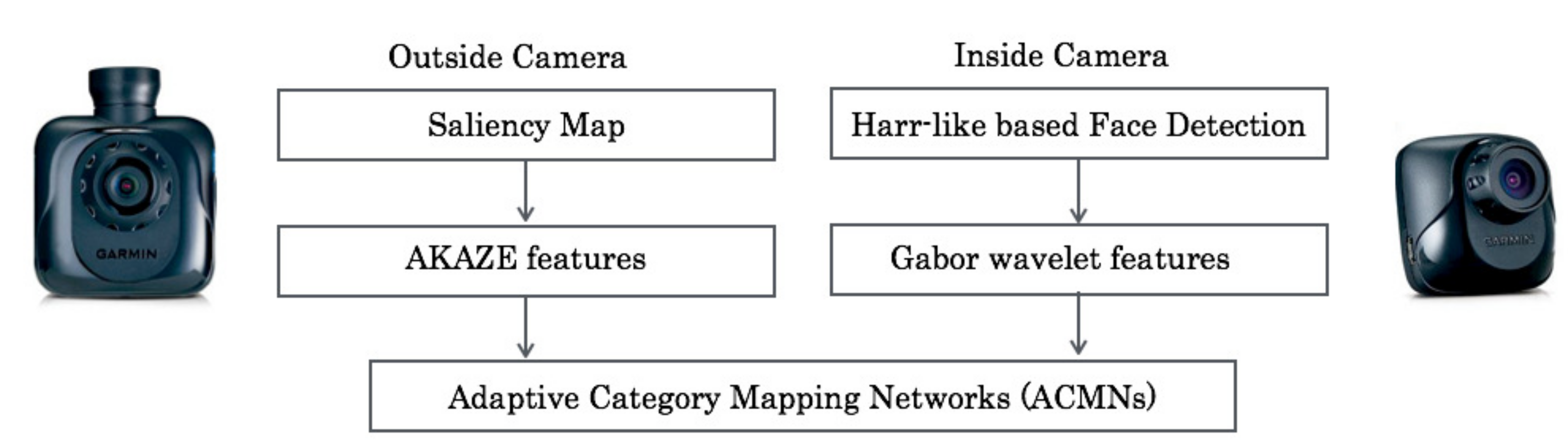
2.1. The Procedure
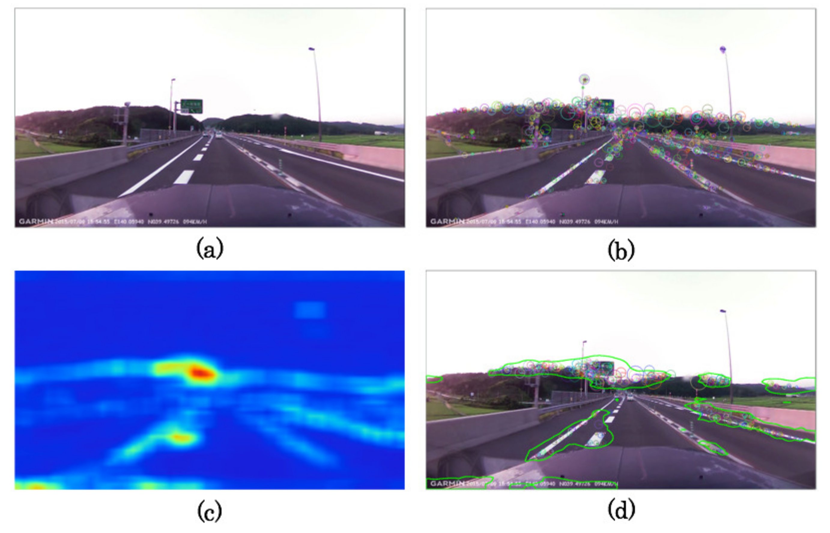
2.2. Saliency Maps
2.3. AKAZE Descriptors
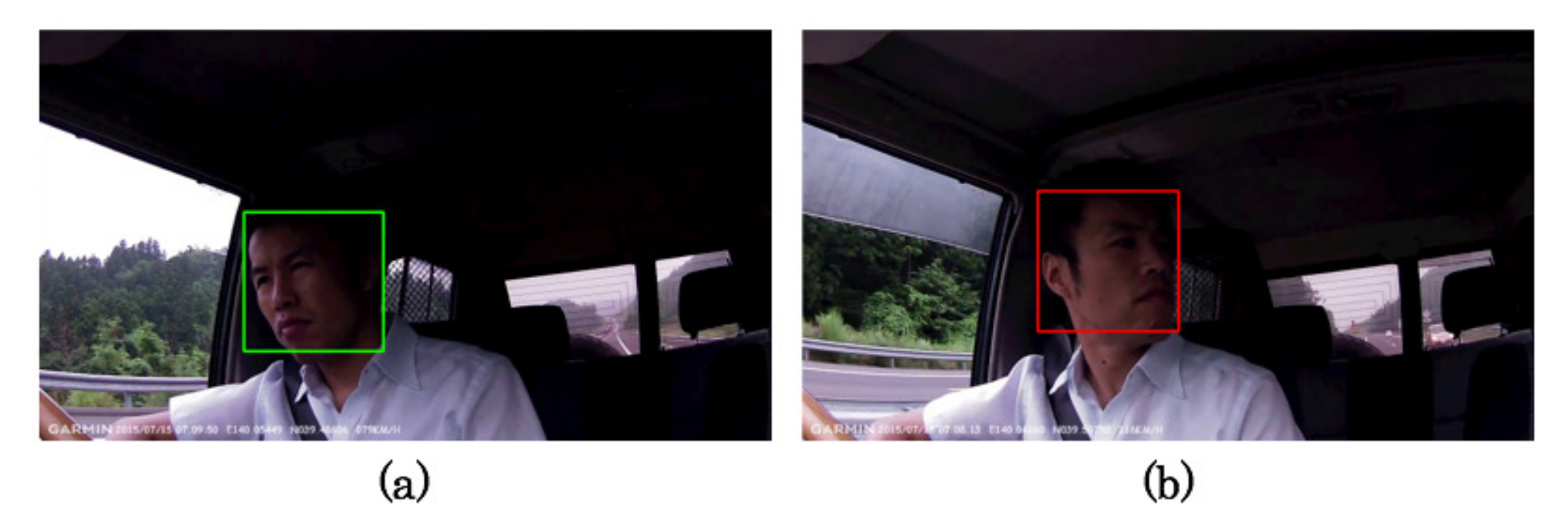
2.4. Face Detection
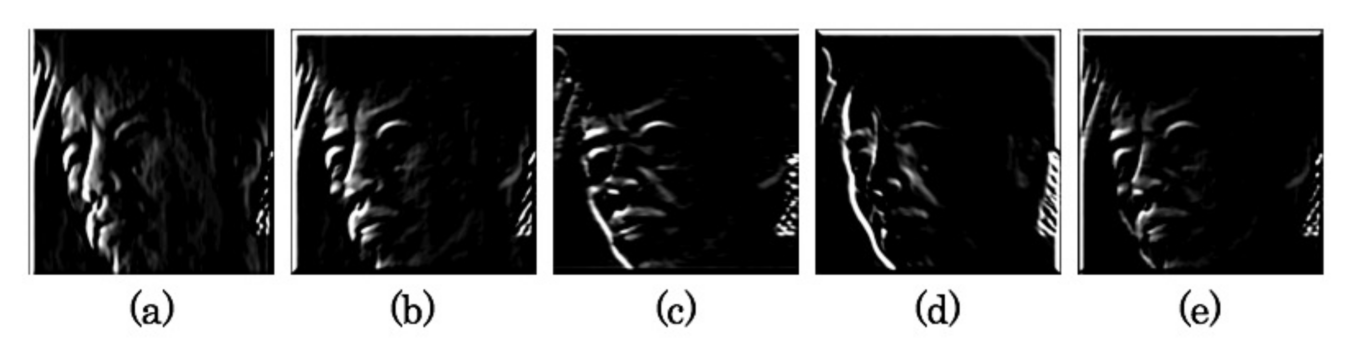
2.5. Gabor Wavelets
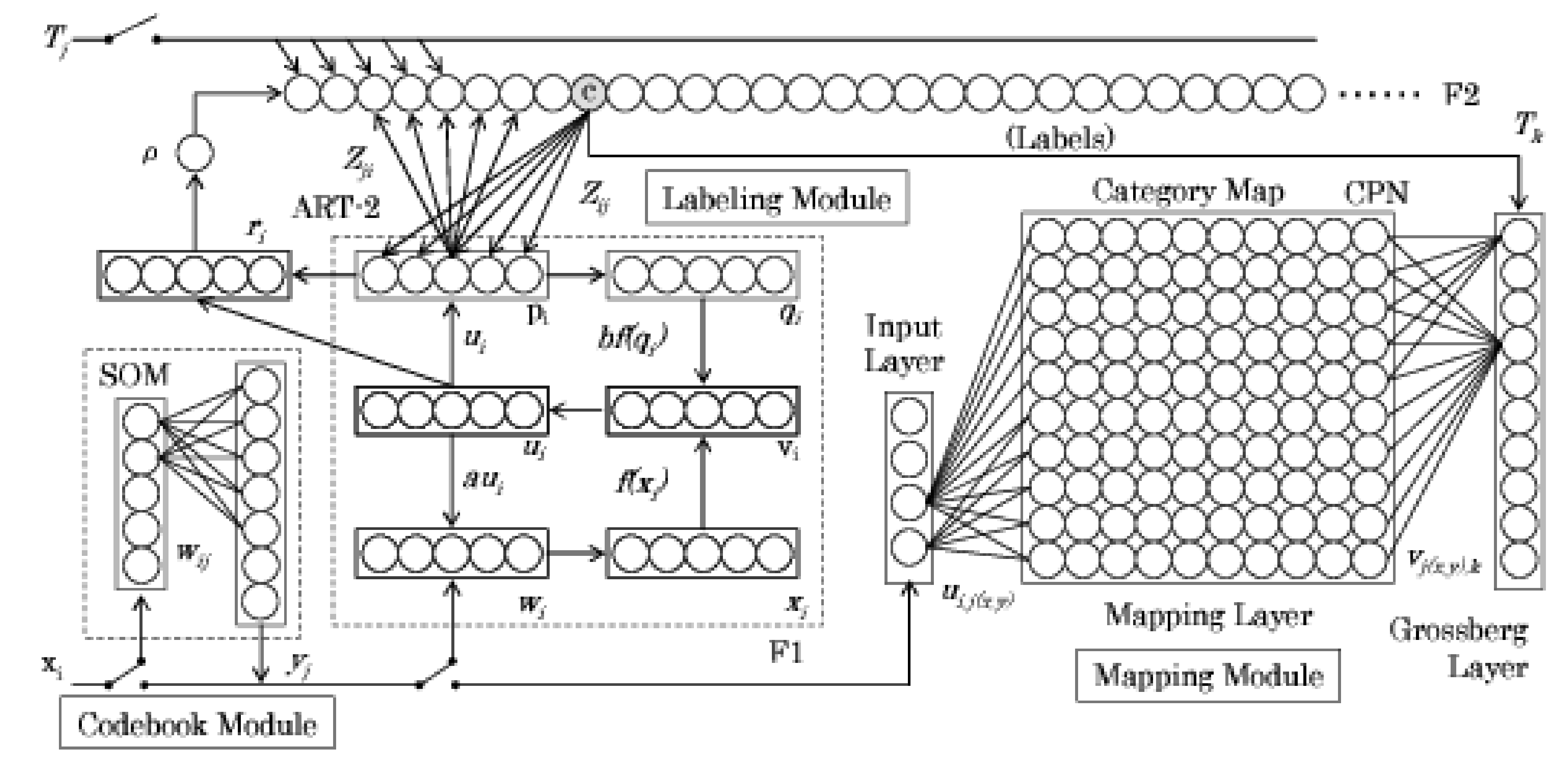
3. Adaptive Category Mapping Networks
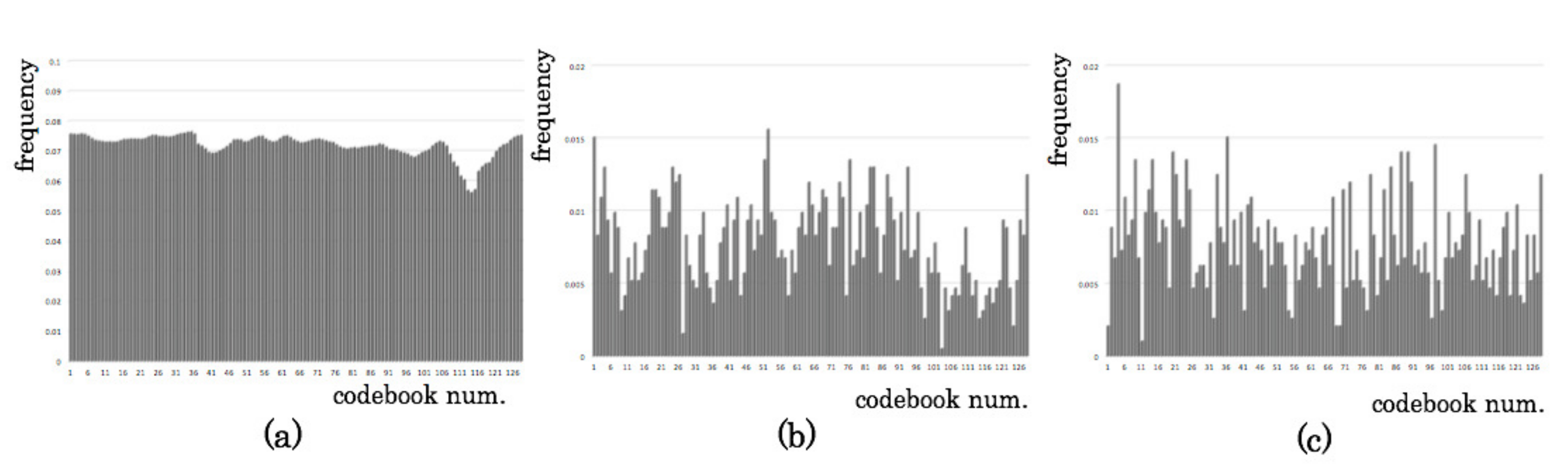
3.1. Codebook Modules
3.2. Labeling Module
3.3. Mapping Module
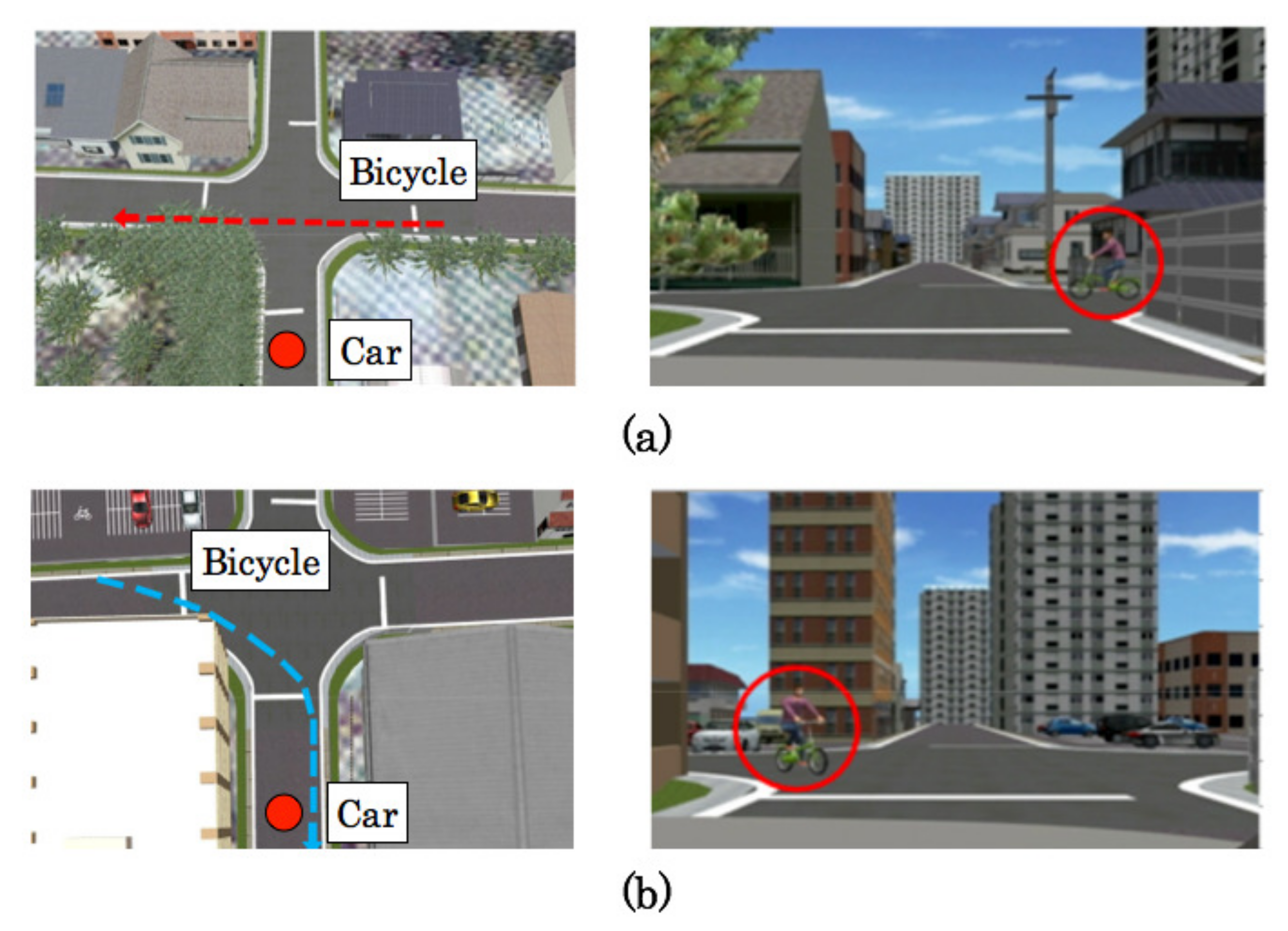
4. Preliminary Experiment Using a Driving Simulator
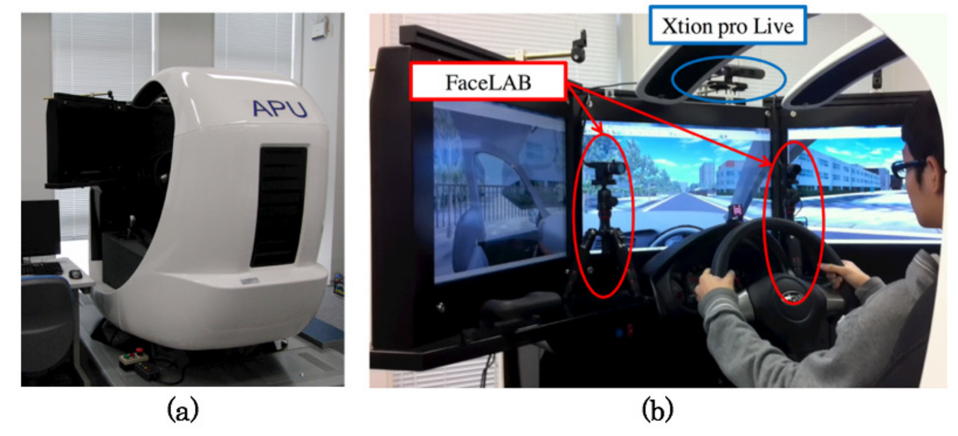
4.1. Measurement Setup
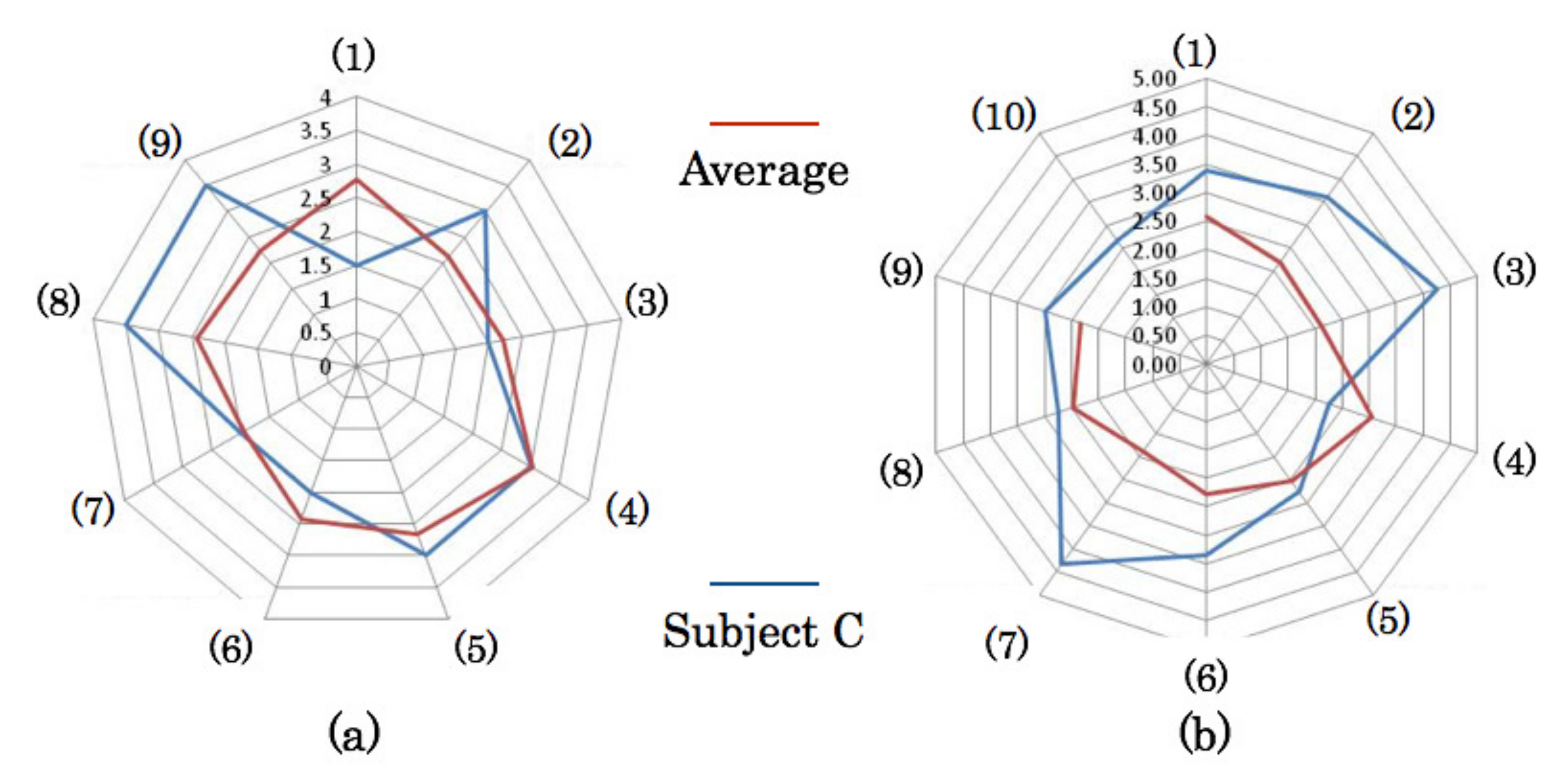
4.2. Driving Characteristics
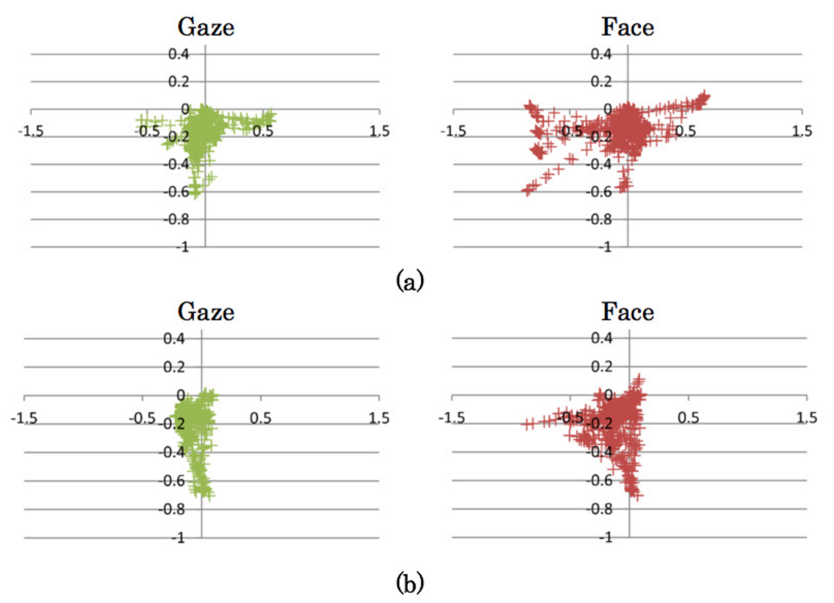
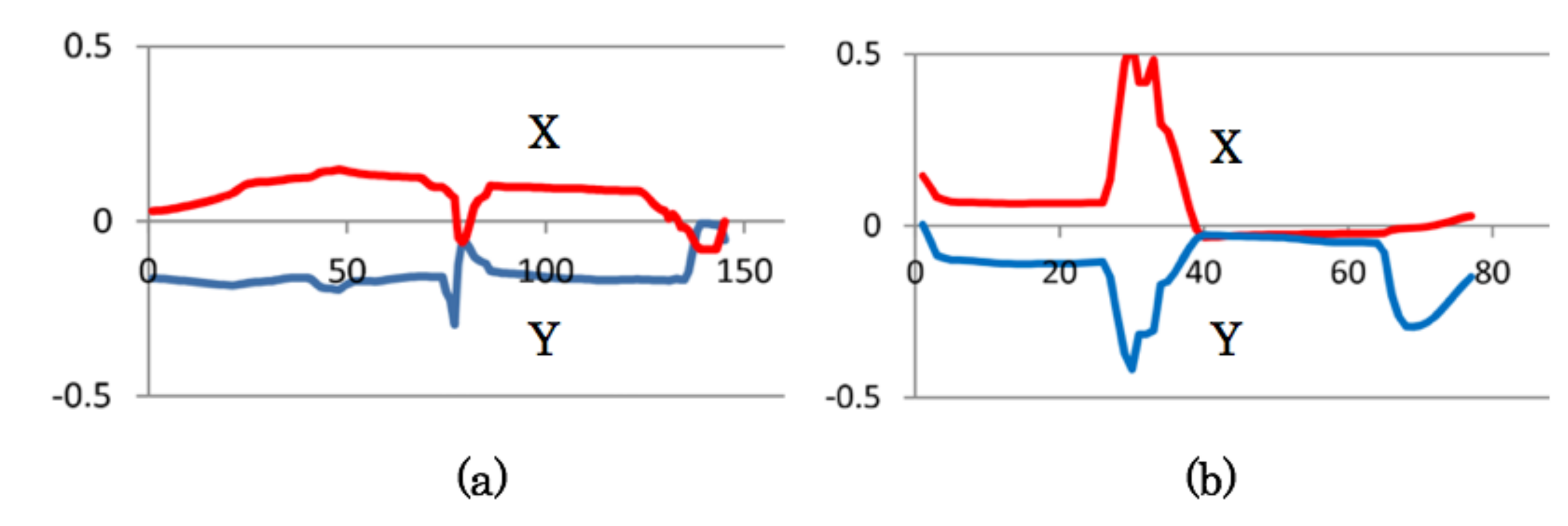
4.3. Measurement Results of Gaze and Face Orientation
4.4. Relation between Near-Miss and Cognitive Distraction
5. Evaluation Experiment Using an Event Data Recorder
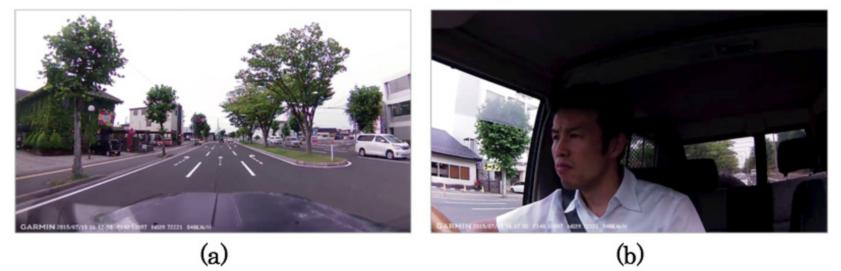
5.1. Experimental Setup
5.2. Feature Extraction Results
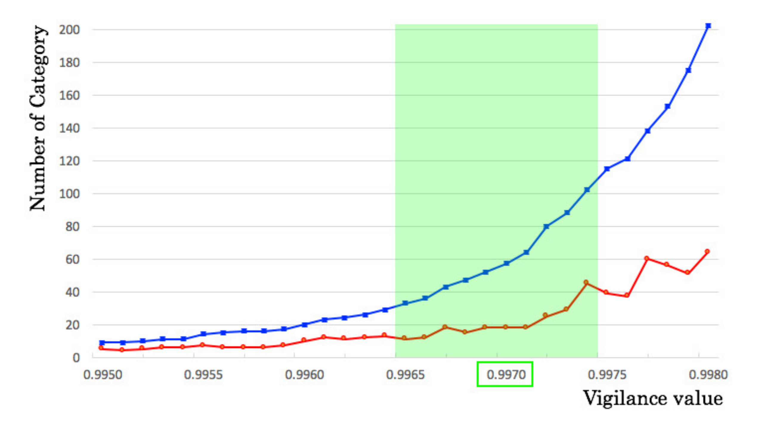
5.3. Classification Granularity
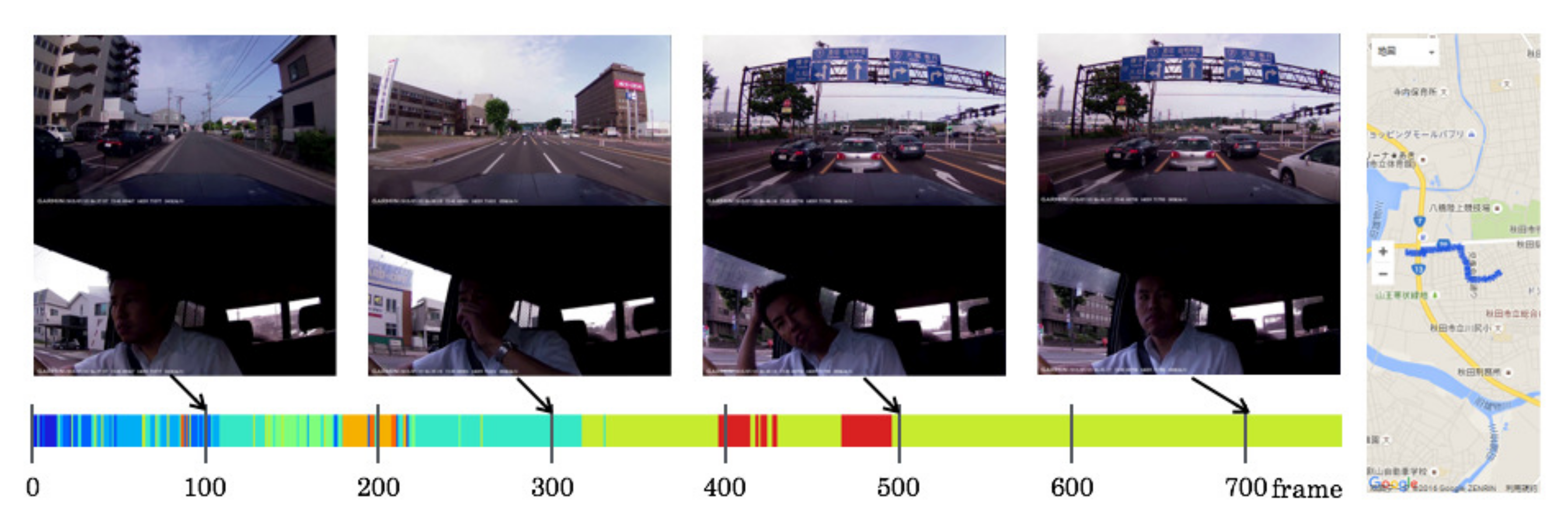
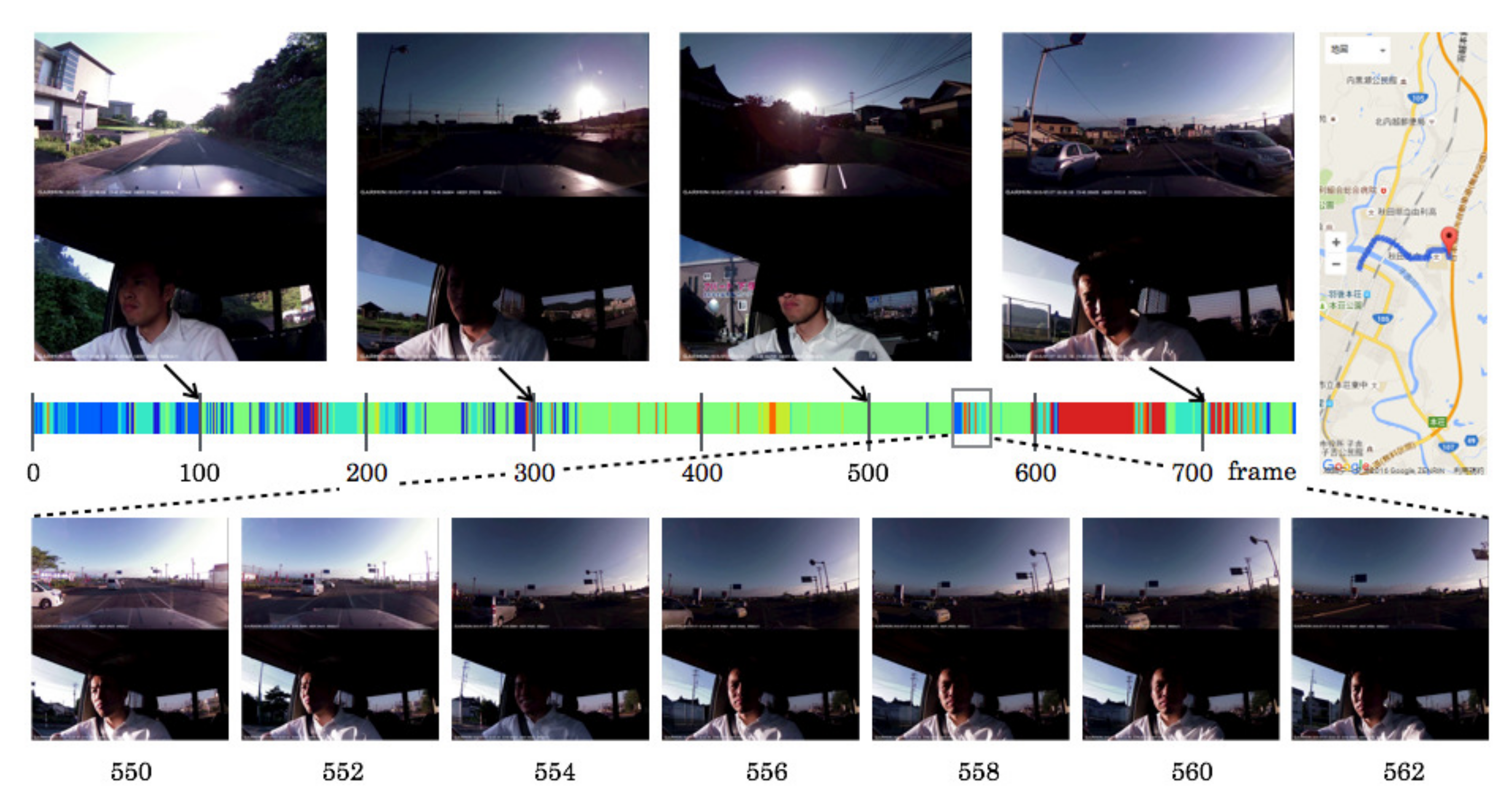
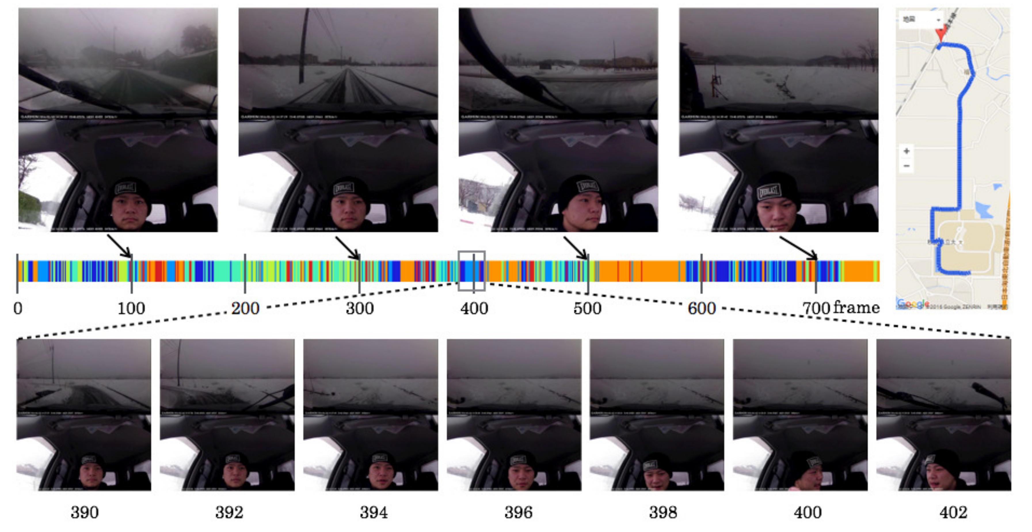
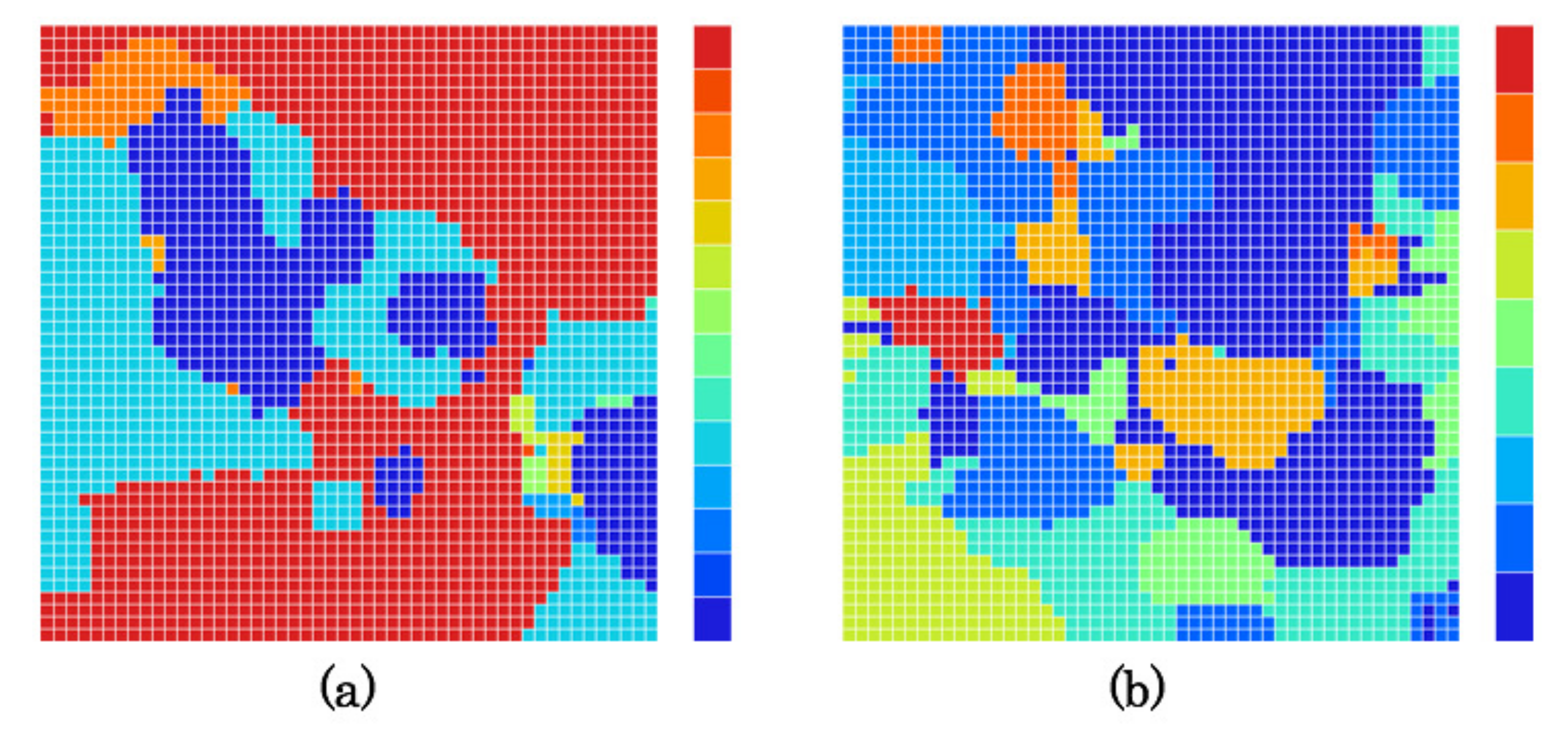
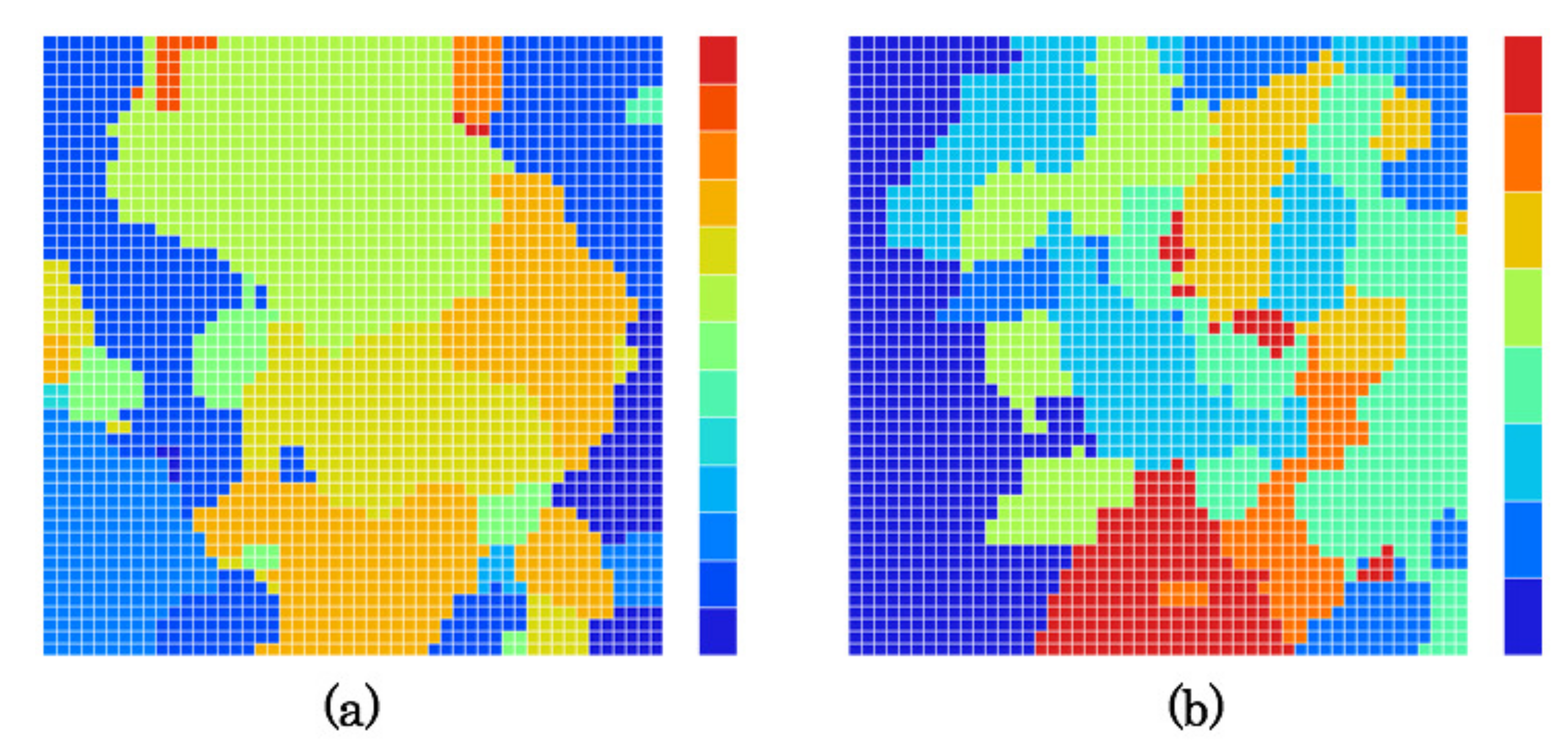
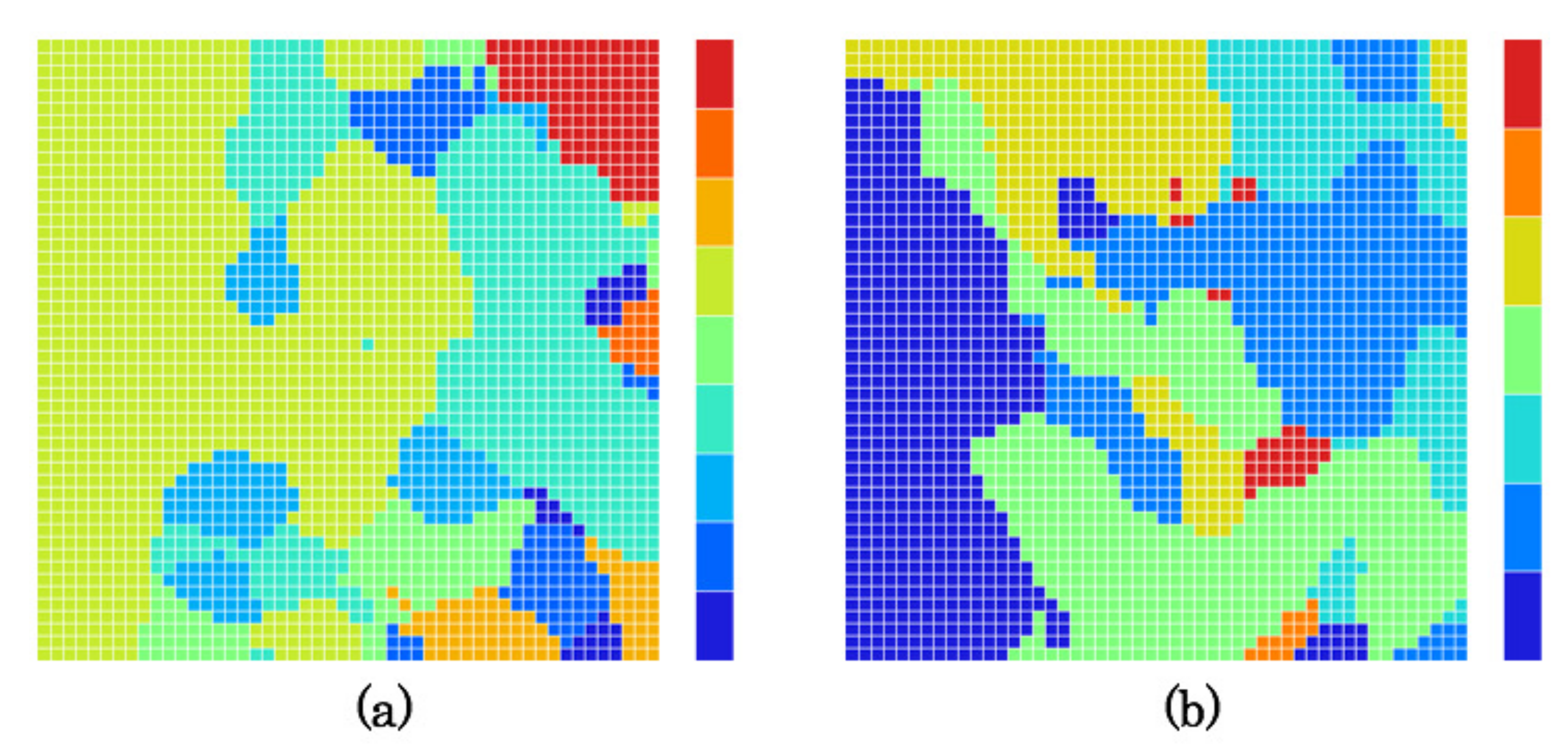
5.4. Created Category Maps
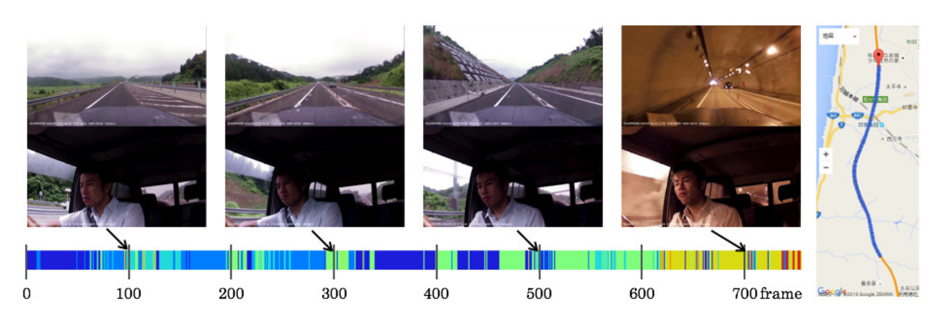
5.5. Driving Episodes with Near-Misses
6. Conclusions
Acknowledgments
Author Contributions
Conflicts of Interest
References
- Woolley, A.W.; Chabris, C.F.; Pentland, A.; Hashmi, N.; Malone, T.W. Evidence for a Collective Intelligence Factor in the Performance of Human Groups. Science 2010, 330, 686–688. [Google Scholar] [CrossRef] [PubMed]
- The Pathway to Driverless Cars: A Detailed Review of Regulations for Automated Vehicle Technologies; Department for Transport: London, UK, 2015.
- Anderson, J.M.; Kalra, N.; Stanley, K.D.; Sorensen, P.; Samaras, C.; Oluwatola, O.A. Autonomous Vehicle Technology: A Guide for Policymakers; RAND Corporation: Santa Monica, CA, USA, 2014. [Google Scholar]
- Obinata, G. Nap Sign Detection during Driving Automobiles. J. Jpn. Soc. Mech. Eng. 2013, 116, 774–777. (In Japanese) [Google Scholar] [CrossRef]
- Uchida, N.; Hu, Z.; Yoshitomi, H.; Dong, Y. Facial Feature Points Extraction for Driver Monitoring System with Depth Camera. Tech. Rep. Inst. Image Inf. Telev. Eng. 2013, 37, 9–12. (In Japanese) [Google Scholar]
- Hirayama, T.; Mase, K.; Takeda, K. Timing Analysis of Driver Gaze under Cognitive Distraction toward Peripheral Vehicle Behavior. In Proceedings of the 26th Annual Conference of the Japanese Society for Artificial Intelligence, Yamaguchi, Japan, 12–15 June 2012; pp. 1–4. (In Japanese). [Google Scholar]
- Terada, Y.; Morikawa, K. Technology for Estimation of Driver: Distracted State with Electroencephalogram. Panasonic Tech. J. 2011, 57, 73–75. (In Japanese) [Google Scholar]
- Matsunaga, J. Facial Expression Recognition Technology to understand the State of Driver. J. Automot. Eng. 2015, 69, 94–97. (In Japanese) [Google Scholar]
- Dong, Y.; Hu, Z.; Uchimura, K.; Murayama, N. Driver Inattention Monitoring System for Intelligent Vehicles: A Review. IEEE Trans. Intell. Transp. Syst. 2011, 12, 596–614. [Google Scholar] [CrossRef]
- Apostoloff, N.; Zelinsky, A. Vision In and Out of Vehicles: Integrated Driver and Road Scene Monitoring. Int. J. Robot. Res. 2004, 23, 513–538. [Google Scholar] [CrossRef]
- Fletcher, L.; Zelinsky, A. Driver Inattention Detection based on Eye Gaze—Road Event Correlation. Int. J. Robot. Res. 2009, 28, 774–801. [Google Scholar] [CrossRef]
- Atance, C.M.; O’Neill, D.K. Episodic future thinking. Trends Cogn. Sci. 2001, 5, 533–539. [Google Scholar] [CrossRef]
- Tulving, E. Episodic Memory: From Mind to Brain. Annu. Rev. Psychol. 2002, 53, 1–25. [Google Scholar] [CrossRef] [PubMed]
- Schacter, D.L.; Benoit, R.G.; Brigard, F.D.; Szpunar, K.K. Episodic Future Thinking and Episodic Counterfactual Thinking: Intersections between Memory and Decisions. Neurobiol. Learn. Mem. 2015, 117, 14–21. [Google Scholar] [CrossRef] [PubMed] [Green Version]
- Maeno, T. How to Make a Conscious Robot: Fundamental Idea based on Passive Consciousness Model. J. Robot. Soc. Jpn. 2005, 23, 51–62. (In Japanese) [Google Scholar] [CrossRef]
- Carpenter, G.A.; Grossberg, S. ART 2: Stable Self-Organization of Pattern Recognition Codes for Analog Input Patterns. Aied Opt. 1987, 26, 4919–4930. [Google Scholar] [CrossRef] [PubMed]
- Kohonen, T. Self-Organizing Maps; Springer Series in Information Sciences; Springer: Berlin, Germany, 1995. [Google Scholar]
- Nielsen, R.H. Counterpropagation networks. Aied Opt. 1987, 26, 4979–4983. [Google Scholar]
- Madokoro, H.; Sato, K.; Nakasho, K.; Shimoi, N. Adaptive Learning Based Driving Episode Description on Category Maps. In Proceedings of the 2017 International Joint Conference on Neural Networks (IJCNN), Anchorage, AK, USA, 14–19 May 2017; pp. 3138–3145. [Google Scholar]
- Itti, L.; Koch, C.; Niebur, E. A Model of Saliency-Based Visual Attention for Rapid Scene Analysis. IEEE Trans. Pattern Anal. Mach. Intell. 1998, 20, 1254–1259. [Google Scholar] [CrossRef]
- Otsu, N. An Automatic Threshold Selection Method Based on Discriminant and Least Squares Criteria. Trans. Inst. Electron. Commun. Eng. Jpn. 1980, J63-D, 349–356. (In Japanese) [Google Scholar]
- Hou, X.; Zhang, L. Saliency Detection: A Spectral Residual Approach. In Proceedings of the IEEE Conference on Computer Vision and Pattern Recognition, Minneapolis, MN, USA, 17–22 June 2007; pp. 1–8. [Google Scholar]
- Rensink, R. Seeing, Sensing, and Scrutinizing. Vis. Res. 2000, 40, 1469–1487. [Google Scholar] [CrossRef]
- Rensink, R.A.; O’Regan, J.K.; Clark, J. To See or not to See: The Need for Attention to Perceive Changes in Scenes. Psychol. Rev. 1997, 8, 368–373. [Google Scholar] [CrossRef]
- Rensink, R.; Enns, J. Preemption Effects in Visual Search: Evidence for Low-Level Grouping. Psychol. Rev. 1995, 102, 101–130. [Google Scholar] [CrossRef] [PubMed]
- Treisman, A.; Gelade, G. A Feature-Integration Theory of Attention. Cogn. Psychol. 1980, 12, 97–136. [Google Scholar] [CrossRef]
- Wolfe, J. Guided Search 2.0: A Revised Model of Guided Search. Psychon. Bull. Rev. 1994, 1, 202–238. [Google Scholar] [CrossRef] [PubMed]
- Oliva, A.; Torralba, A. Modeling the Shape of the Scene: A Holistic Representation of the Spatial Envelope. Int. J. Comput. Vis. 2001, 42, 145–175. [Google Scholar] [CrossRef]
- Lowe, D.G. Object Recognition from Local Scale-Invariant Features. In Proceedings of the Seventh IEEE International Conference on Computer Vision, Kerkyra, Greece, 20–27 September 1999; pp. 1150–1157. [Google Scholar]
- Alcantarilla, P.F.; Bartoli, A.; Davison, A.J. KAZE Features. Lect. Notes Comput. Sci. 2012, 7577, 214–227. [Google Scholar]
- Alcantarilla, P.F.; Nuevo, J.; Bartoli, A. Fast Explicit Diffusion for Accelerated Features in Nonlinear Scale Spaces. In Proceedings of the 24th British Machine Vision Conference, Bristol, UK, 9–13 September 2013. [Google Scholar]
- Scharr, H. Optimal Operators in Digital Image Processing; Heidelberg University: Heidelberg, Germany, 2000. [Google Scholar]
- Weickert, J.; Scharr, H. A Scheme for Coherence-Enhancing Diffusion Filtering with Optimized Rotation Invariance. J. Vis. Commun. Image Represent. 2002, 13, 103–118. [Google Scholar] [CrossRef]
- Yang, X.; Cheng, K.T. LDB: An Ultra-Fast Feature for Scalable Augmented Reality. In Proceedings of the 2012 IEEE International Symposium on Mixed and Augmented Reality (ISMAR), Atlanta, GA, USA, 5–8 November 2012; pp. 49–57. [Google Scholar]
- Perona, P.; Malik, J. Scale-Space and Edge Detection Using Anisotropic Diffusion. IEEE Trans. Pattern Anal. Mach. Intell. 1990, 12, 1651–1686. [Google Scholar] [CrossRef]
- Viola, P.; Jones, M. Rapid Object Detection Using a Boosted Cascade of Simple Features. Comput. Vis. Pattern Recognit. 2001, 1, 511–518. [Google Scholar]
- Rowley, H.; Baluja, S.; Kanade, T. Neural Network-Based Face Detection. IEEE Trans. Pattern Anal. Mach. Intell. 1998, 20, 22–38. [Google Scholar] [CrossRef]
- Papageorgiou, C.; Oren, M.; Poggio, T. A General FrameWork for Object Detection. In Proceedings of the Sixth International Conference on Computer Vision (IEEE Cat. No.98CH36271), Bombay, India, 4–7 January 1998. [Google Scholar]
- Haar, A. Zur Theorie der Orthogonalen Funktionensysteme. Math. Ann. 1910, 69, 331–371. (In German) [Google Scholar] [CrossRef]
- Freund, Y.; Schapire, R.E. A Decision-Theoretic Generalization of On-Line Learning and an Aication to Boosting. J. Comput. Syst. Sci. 1997, 55, 119–139. [Google Scholar] [CrossRef]
- Schapire, R.E.; Freund, Y. Boosting: Foundations and Algorithms; The MIT Press: Cambridge, MA, USA, 2012. [Google Scholar]
- Amari, S. Encyclopedia of Brain Sciences; Asakurashoten Press: Tokyo, Japan, 2000. (In Japanese) [Google Scholar]
- Hubel, D.H.; Wiesel, T.N. Functional Architecture of Macaque Monkey Visual Cortex. Proc. R. Soc. B 1978, 198, 1–59. [Google Scholar] [CrossRef]
- Lee, T.S. Image representation using 2D Gabor wavelets. IEEE Trans. Pattern Anal. Mach. Intell. 1996, 18, 959–971. [Google Scholar]
- Madokoro, H.; Shimoi, N.; Sato, K. Adaptive Category Mang Networks for All-Mode Topological Feature Learning Used for Mobile Robot Vision. In Proceedings of the 23rd IEEE International Symposium on Robot and Human Interactive Communication (RO-MAN), Edinburgh, UK, 25–29 August 2014; pp. 678–683. [Google Scholar]
- Sudo, A.; Sato, A.; Hasegawa, O. Associative Memory for Online Learning in Noisy Environments Using Self-Organizing Incremental Neural Network. IEEE Trans. Neural Netw. 2009, 20, 964–972. [Google Scholar] [CrossRef] [PubMed]
- Csurka, G.; Dance, C.R.; Fan, L.; Willamowski, J.; Bray, C. Visual Categorization with Bags of Keypoints. In Proceedings of the ECCV Workshop Statistical Learning Computer Vision, Prague, Czech Republic, 16 May 2004; pp. 1–22. [Google Scholar]
- McQueen, J. Some Methods for Classification and Analysis of Multivariate Observations. In Proceedings of the Fifth Berkeley Symposium on Mathematical Statistics and Probability: Statistics; University of California Press: Berkeley, CA, USA, 1967; pp. 281–297. [Google Scholar]
- Vesanto, J.; Alhoniemi, E. Clustering of the Self-Organizing Map. IEEE Trans. Neural Netw. 2000, 11, 586–600. [Google Scholar] [CrossRef] [PubMed]
- Terashima, M.; Shiratani, F.; Yamamoto, K. Unsupervised Cluster Segmentation Method Using Data Density Histogram on Self-Organizing Feature Map. Trans. Inst. Electron. Inf. Commun. Eng. 1996, J79-D-II, 1280–1290. (In Japanese) [Google Scholar]
- Carpenter, G.A.; Grossberg, S. Pattern Recognition by Self-Organizing Neural Networks; The MIT Press: Cambridge, MA, USA, 1991. [Google Scholar]
- Sato, K.; Ito, M.; Madokoro, H.; Kadowaki, S. Driver Body Information Analysis for Distraction State Detection. In Proceedings of the IEEE International Conference on Vehicular Electronics and Safety (ICEVS2015), Yokohama, Japan, 5–7 November 2015. [Google Scholar]
- Suenaga, O.; Nakamura, Y.; Liu, X. Fundamental Study of Recovery Time from External Information Processing while Driving Car. Jpn. Ergon. Soc. Ergon. 2015, 51, 62–70. (In Japanese) [Google Scholar] [CrossRef]
- Abe, K.; Miyatake, H.; Oguri, K. Induction and Biosignal Evaluation of Tunnel Vision Driving Caused by Sub-Task. Trans. Inst. Electron. Inf. Commun. Eng. A 2008, J91-A, 87–94. [Google Scholar]
- Ishibahi, M. HQL Manual of Driving Style Questionnaires; Research Institute of Human Engineering for Quality Life: Tsukuba, Japan, 2003. (In Japanese) [Google Scholar]
- Ishibahi, M. HQL Manual of Driving Workload Sensibility Questionnaires; Research Institute of Human Engineering for Quality Life: Tsukuba, Japan, 2003. (In Japanese) [Google Scholar]
- Regan, M.A.; Lee, J.D.; Young, K.L. Driver Distraction: Theory, Effects, and Mitigation; CRC Press: Boca Raton, FL, USA, 2008. [Google Scholar]
- Hynd, D.; McCarthy, M. Study on the Benefits Resulting from the Installation of Event Data Recorders; Project Report PRP707; Transport Research Laboratory: Wokingham, UK, 2014. [Google Scholar]


| Size (front) | 82 × 66 × 42 mm |
| Size (rear) | 46 × 46 × 46 mm |
| Weight (front) | 122 g |
| Weight (rear) | 37 g |
| Imaging device | CMOS |
| Resolution | 3 million pixel |
| Frame rate | 30 fps |
| View angle | diagonal 132 |
| (horizontal 120) | |
| Focal length | F2.0 |
| Embedded sensors | Gyroscope, GPS, and TLS |
| Case | Near-Miss | Situation | Season |
|---|---|---|---|
| I | rushing out | evening | summer |
| II | slip | snow | winter |
© 2018 by the authors. Licensee MDPI, Basel, Switzerland. This article is an open access article distributed under the terms and conditions of the Creative Commons Attribution (CC BY) license (http://creativecommons.org/licenses/by/4.0/).
Share and Cite
Madokoro, H.; Sato, K.; Shimoi, N. Category Maps Describe Driving Episodes Recorded with Event Data Recorders. Mach. Learn. Knowl. Extr. 2019, 1, 43-63. https://doi.org/10.3390/make1010003
Madokoro H, Sato K, Shimoi N. Category Maps Describe Driving Episodes Recorded with Event Data Recorders. Machine Learning and Knowledge Extraction. 2019; 1(1):43-63. https://doi.org/10.3390/make1010003
Chicago/Turabian StyleMadokoro, Hirokazu, Kazuhito Sato, and Nobuhiro Shimoi. 2019. "Category Maps Describe Driving Episodes Recorded with Event Data Recorders" Machine Learning and Knowledge Extraction 1, no. 1: 43-63. https://doi.org/10.3390/make1010003
APA StyleMadokoro, H., Sato, K., & Shimoi, N. (2019). Category Maps Describe Driving Episodes Recorded with Event Data Recorders. Machine Learning and Knowledge Extraction, 1(1), 43-63. https://doi.org/10.3390/make1010003