Analysis of Machine Learning Algorithms for Opinion Mining in Different Domains

Abstract

Sentiment classification (SC) is a reference to the task of sentiment analysis (SA), which is a subfield of natural language processing (NLP) and is used to decide whether textual content implies a positive or negative review. This research focuses on the various machine learning (ML) algorithms which are utilized in the analyzation of sentiments and in the mining of reviews in different datasets. Overall, an SC task consists of two phases. The first phase deals with feature extraction (FE). Three different FE algorithms are applied in this research. The second phase covers the classification of the reviews by using various ML algorithms. These are Naïve Bayes (NB), Stochastic Gradient Descent (SGD), Support Vector Machines (SVM), Passive Aggressive (PA), Maximum Entropy (ME), Adaptive Boosting (AdaBoost), Multinomial NB (MNB), Bernoulli NB (BNB), Ridge Regression (RR) and Logistic Regression (LR). The performance of PA with a unigram is the best among other algorithms for all used datasets (IMDB, Cornell Movies, Amazon and Twitter) and provides values that range from 87% to 99.96% for all evaluation metrics.

1. Introduction

Sentiment analysis, also known as opinion mining (OM), is defined as figuring out the public attitude of individuals toward distinct topics and news [1]. It is also the computational handling of opinions, feelings, and the subjectivity of textual content [2]. Nowadays, individuals inspect feedback and online posts about any product—which are called opinions, emotions, feelings, attitudes, considerations, beliefs or conduct of clients—before purchasing it. Sentiment analysis is the task of automatically classifying the sentiment orientation (positive or negative) of a textual content. It can be used to classify online products as recommended or not recommended (satisfied or not satisfied) [3].

There are two fundamental OM approaches used to decide whether the review or audit sentences are positive or negative [4]. The first approach is a machine learning (ML) approach which is very frequently used in sentiment analysis (SA), as this approach is based on supervised, unsupervised, and semi-supervised learning. In supervised learning, the dataset is labeled to acquire a reasonable and sensible output. Dissimilar to supervised learning, the unsupervised learning process does not have any need for labeled data. In order to tackle the issue of processing unlabeled data, clustering algorithms are utilized [5]. The second approach makes use of a present lexicon or dictionary with words, expressions, or phrases—terms labeled either positive or negative [6,7]. These approaches were performed based on real-life needs. This study presents the impact of supervised learning algorithms on different labeled datasets.

Binary sentiment classification (SC) and multi-class SC are the very regularly used methodologies of SC [8]. Each document or feedback review of the dataset is classified into two main classes, which are a positive or a negative sentiment in binary SC [9]. Whereas in multi-class SC each document could be classified into more than two classes, a degree of the sentiment could be a solid positive, positive, neutral, negative or solid negative [10].

SA is categorized into three main levels—the aspect or feature level (AL), the sentence level (SL) and the document level (DL) [11]. The AL refers to classify the sentiments that are expressed on various features or aspects of an entity. In the SL, the fundamental concern is to pick whether each sentence infers a positive, negative or neutral opinion. In the DL, the basic concern is to classify whether the whole opinion in a document implies a positive or negative sentiment. The SL and DL analyses are insufficient to precisely monitor what people accept and reject. This research focuses on the document level of sentiment analysis.

The rest of this paper is organized as follows: Section 2 presents a literature review of SA. Section 3 demonstrates the characteristics of the different datasets. In Section 4, the proposed methodology of SA is clarified. Section 5 discusses the results of the proposed methodology on different datasets. Section 6 concludes the research and introduces the scope and extension for future work.

2. Literature Review

In this section the related work is presented. It was investigated in various domains such as movie reviews, product reviews, and Twitter.

Tripathy et al. [5] did a study on classifying movie reviews using different ML algorithms, which are naïve bayes (NB), maximum entropy (ME), stochastic gradient descent (SGD), and support vector machine (SVM). These algorithms are carried out on the IMDB dataset using different combinations between n-gram approaches, for example, unigram and bigram, bigram and trigram, and unigram, bigram and trigram. Their results show that support vector machines (SVM) acquired the highest accuracy with 88.9% when unigram, bigram and trigram are applied as feature extraction.

Deng et al. [12] applied SVM combined with Importance of a Term in a Document (ITD) in order to extract features on various datasets, which are the Cornell movie reviews, Amazon products reviews and the Stanford movie reviews. Their approach certainly beats Best Matching (BM25) on two of three datasets while the distinction is indistinctive on the small Cornell movie review dataset with an accuracy of 88.50%. The accuracy of the combined algorithm is 87.44% on the Stanford movie review data set, which is greater than the BM25 (87.10%). Furthermore, the accuracy of the combined algorithm is 88.70% on Amazon products reviews.

Suresh and Raj [13] exhibited a novel model for Twitter SA of a specific product and have analyzed the four usually used supervised ML algorithms (NB, Decision Tree J48, SVM and ME). Among those applied algorithms, results show that the J48 algorithm ended up being the most efficient ML algorithm, in contrast with the other three algorithms, with an overall accuracy of 92%.

Joshi and Vekariya [14] presented a practical approach to Twitter SA. The SVM algorithm with Part of Speech (POS) performs very well in SA with an accuracy of 92%.

Wawre and Deshmukh [15] compared two supervised ML algorithms (NB and SVM) for SA on the IMDB movie reviews dataset. The NB is 65.57% accurate compared with SVM with an accuracy of 45.71%.

Liu et al. [16] introduced a fundamental framework for SA on the Cornell movie review dataset utilizing NB with the Hadoop framework. The results show that the NB classifier could scale up enough. The accuracy achieved is below 82%.

In addition to machine learning based sentiment analysis, there are other approaches for SA that are based on lexicon. Many researchers applied sentiment analysis using a dictionary or corpus [6,7].

3. Datasets

Four different datasets were examined—the IMDB dataset [17], the Cornell dataset [18], the Amazon products dataset [19], and the Twitter dataset [20,21]. All these English reviews datasets are balanced and only contain two sentiment classes, which are positive and negative sentiments.

The first dataset, IMDB movie review, was initially used by Reference [22], then it was used and expanded widely as a benchmark dataset. The polarity dataset contains 12,500 positive and 12,500 negative processed reviews of movies, which were extracted from the internet movie database with an average of 30 sentences in each document.

The second data set is also a movie reviews dataset collected from Cornell movie reviews [23]. It includes 1000 positive and 1000 negative movie reviews. The number of positive words is 372,016 while the number of the distinct positive words is 29,693. The number of negative words is 330,463 while the number of the distinct negative words is 27,749.

The third dataset is collected from Amazon product reviews. The dataset has 1000 reviews divided into 500 positive and 500 negative. This dataset contains 981 distinct positive words and 1125 distinct negative words out of a total number of 5180 words.

Finally, the last dataset used is a Twitter dataset. It contains more than 1,500,000 processed tweets. However, in this research only 150,000 tweets are used for training and testing. The characteristics of used datasets can be illustrated in

Table 1. Characteristics of different datasets.

	Dataset	IMDB	Cornell Movies	Amazon	Tweets
Term
Positive		12,500	1000	500	75 K
Negative		12,500	1000	500	75 K
Total		25 K	2000	1000	150 K

.

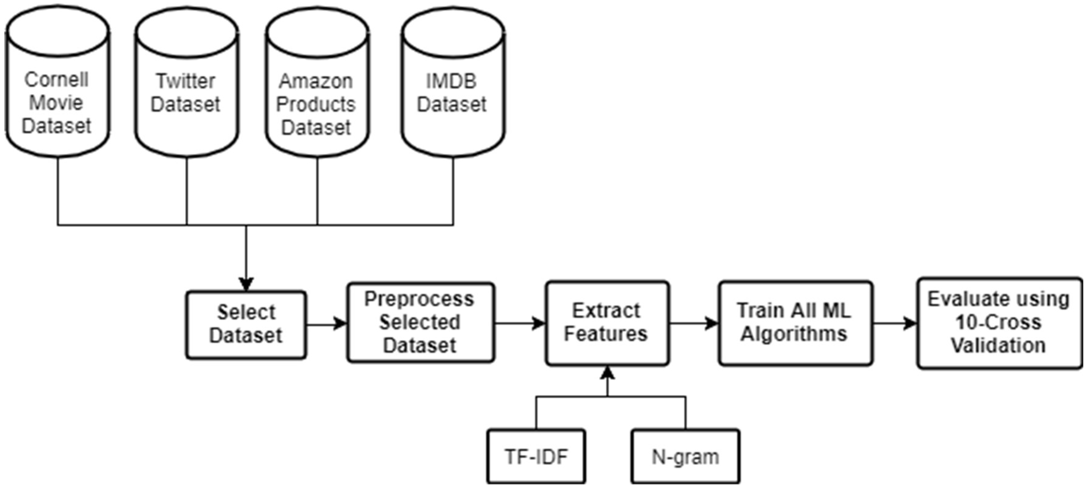
4. The Proposed Methodology

In this research, experiments are implemented with respect to binary SC, since this classification is important for many users who want to make a decision either to buy a product or not, watch a movie or not and so on. The proposed methodology for SA is a five-step process. In the first step, a dataset is selected from among the four different datasets. Pre-processing is performed in the second step, while the third step involves the FE algorithms that are applied on the selected dataset. Next, all ML algorithms are trained. Finally, the different ML algorithms are evaluated using 10-fold. The proposed methodology is illustrated in Figure 1.

4.1. Datasets Pre-Processing

The reviews datasets contain a lot of feedback and opinions which are expressed in various ways by clients. The four datasets utilized in this work are already labeled. Labeled datasets have a negative and positive polarity. The raw data having polarity is extremely susceptible to inconsistency, irregularity and redundancy. The structure of the data influences the results. To enhance the quality and performance of the classification process, the raw data needs to be pre-processed [24]. The pre-processing task deals with the preparation process that removes the repetitive words, non-English characters and punctuations. It enhances the proficiency and adeptness of the data. It includes removing non-English letters, tokenizing, removing stop words, removing repeated characters, removing URLs and user mentions, removing hashtags and retweets for the Twitter dataset, and handling emoticons [25,26].

4.2. Feature Extraction

In order to apply ML algorithms to the SA datasets, it is essential to extract confident features from the textual content that lead to a successful correct classification. The original textual content data are typically presented as an element of a Feature Set (FS), FS = (feature 1, feature 2 … feature n). In this research, two FE algorithms are applied, these are Term Frequency–Inverse Document Frequency (TF–IDF) and N-gram.

4.2.1. Term Frequency–Inverse Document Frequency Algorithm

The Term Frequency–Inverse Document Frequency (TF–IDF) algorithm is a regular measurement utilized as a part of the textual content classification framework. TF–IDF contains two factors—term frequency and inverse document frequency. Term frequency is exposed through the basic monitoring of the frequency of a given expression that has occurred in a given document. The inverse document frequency is calculated by dividing the number of all documents by the total number of documents that a given word is stated in. When these factors are multiplied together, the output score is the value that is the highest for words that appear frequently in documents and lowest for terms that appear frequently in each document. This allows us to find terms that are significant and weighty in a document [27].

4.2.2. N-Gram Algorithm

N-gram would fit for capturing textual context to some scope and is broadly used in NLP tasks. Whether to apply a higher order of n-gram is beneficial or not can be debated. Many researchers say that the unigram performs better than the bigram in classifying movie reviews by sentiment polarity, however different analysts and researchers found that in the different reviews dataset, bigrams and trigrams outperform unigrams [28].

4.3. Machine Learning Classification

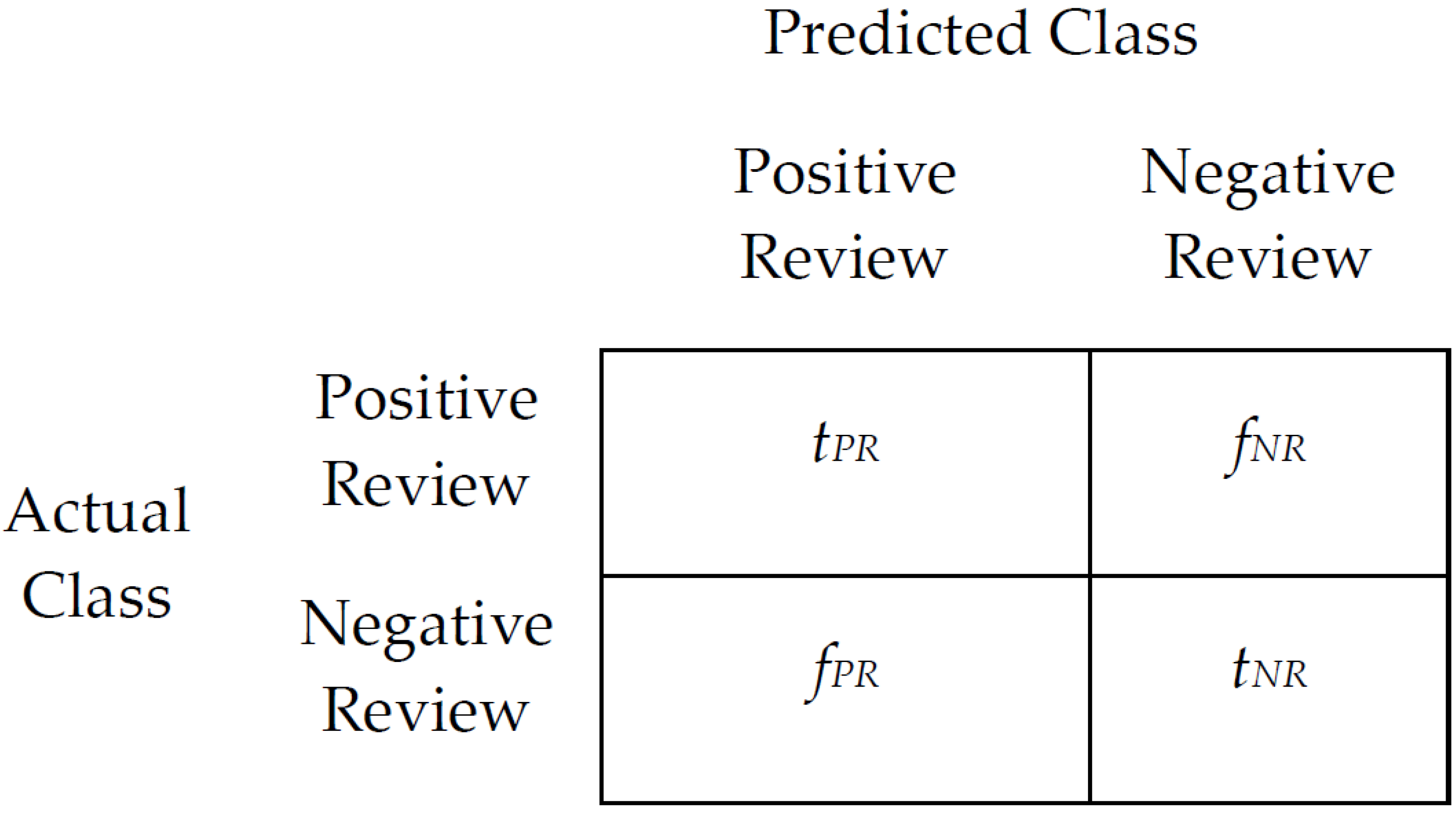
In this research, different ML algorithms are applied to four different datasets to determine their efficiency and applicability for text classification and compare their evaluation accuracies [29,30,31]. The different ML algorithms are NB, SGD, SVM, Passive Aggressive (PA), Maximum Entropy, Adaptive Boosting (AdaBoost), Multinomial Naïve Bayes (MNB), Bernoulli Naïve Bayes (BNB), Ridge Regression (RR) and Logistic Regression (LR). The motive behind utilizing such algorithms is their viable capability to manage and deal with textual categorizations, in which the quantity of features is very extensive. The experiments have been conducted using Python 3.6 libraries. The two Python libraries used for the experiments are Scikit-learn [32] and Natural Language Tool Kit (NLTK) [33]. These libraries are free and grant researchers the ability to employ ML algorithms.

4.4. Evaluation

K-fold-cross-validation is conducted in the experiments of various ML algorithms. In this research the 10-fold cross validation is used to evaluate the ML algorithms’ performance [34]. The confusion matrix of the evaluation metrics is shown in Figure 2 where t_PR stands for true positive review, t_NR stands for true negative review, f_PR stands for false positive review, and f_NR stands for false negative review.

The Precision (Prc.), Recall (Rcl.), Accuracy (Acc.) and F-score (F-s) are calculated to measure the performance of the applied algorithms. The equations of Prc., Rcl., Acc. and F-s are defined in Equations (1)–(4).

$$\mathrm{Prc}.=\frac{t_{PR}}{t_{PR}+f_{PR}}$$

(1)

$$\mathrm{Rcl}.=\frac{t_{PR}}{t_{PR}+f_{NR}}$$

(2)

$$\mathrm{Acc}.=\frac{\mathrm{No}.\mathrm{of}\mathrm{Correctly}\mathrm{Classified}\mathrm{Reviews}}{\mathrm{Total}\mathrm{No}.\mathrm{of}\mathrm{Reviews}}$$

(3)

$$\text{F-s}=\frac{2\times \mathrm{Prc}.\times \mathrm{Rcl}.}{\mathrm{Prc}.+\mathrm{Rcl}.}$$

(4)

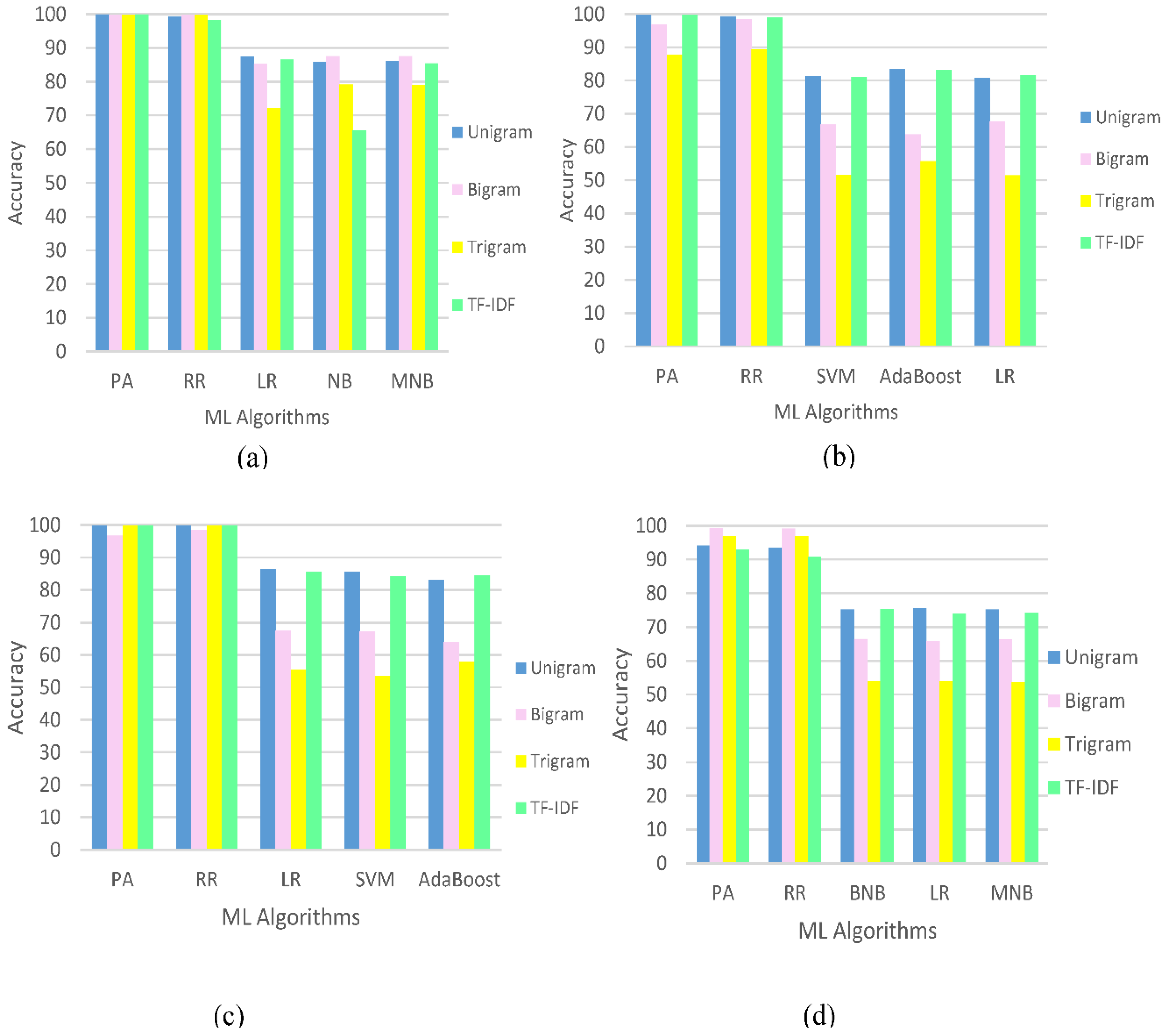
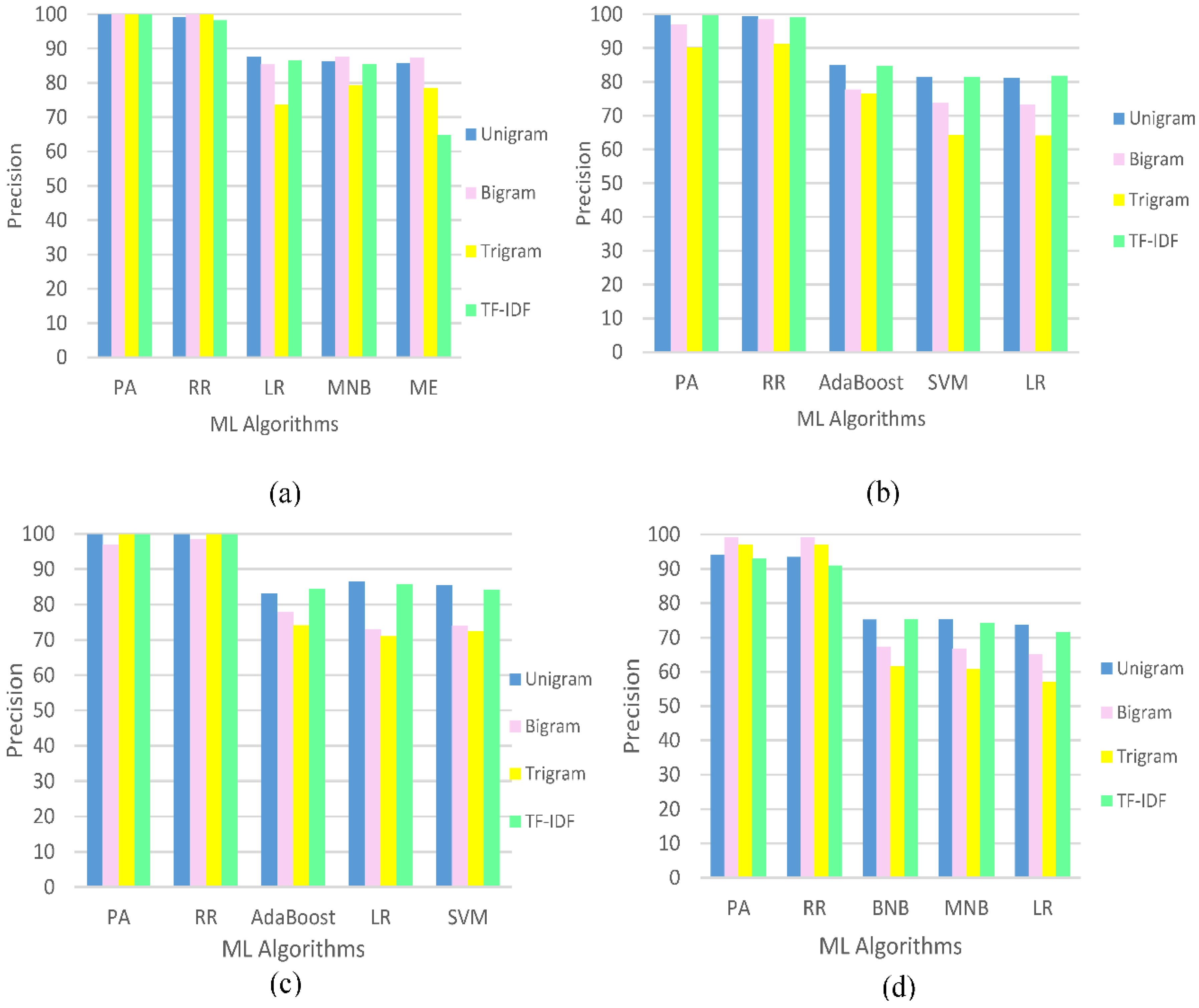
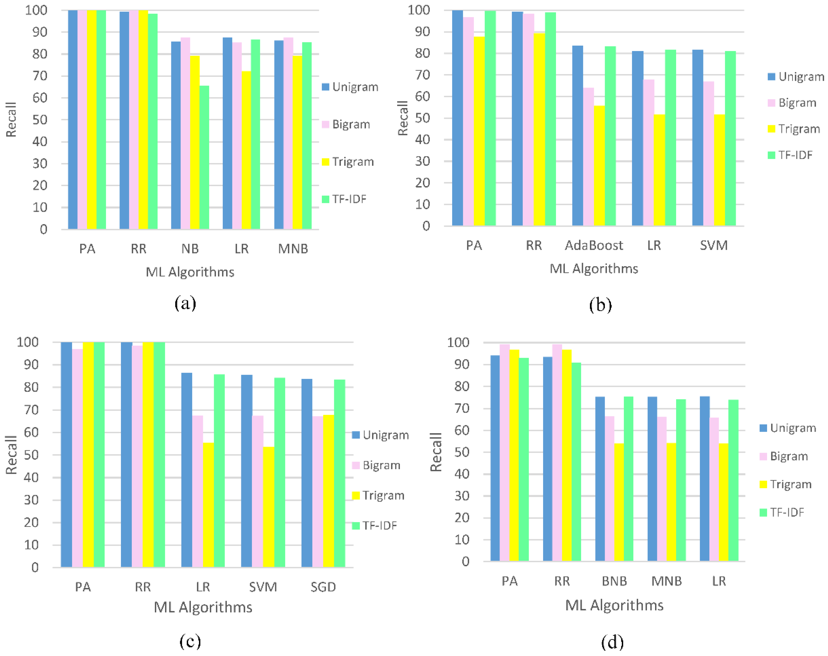
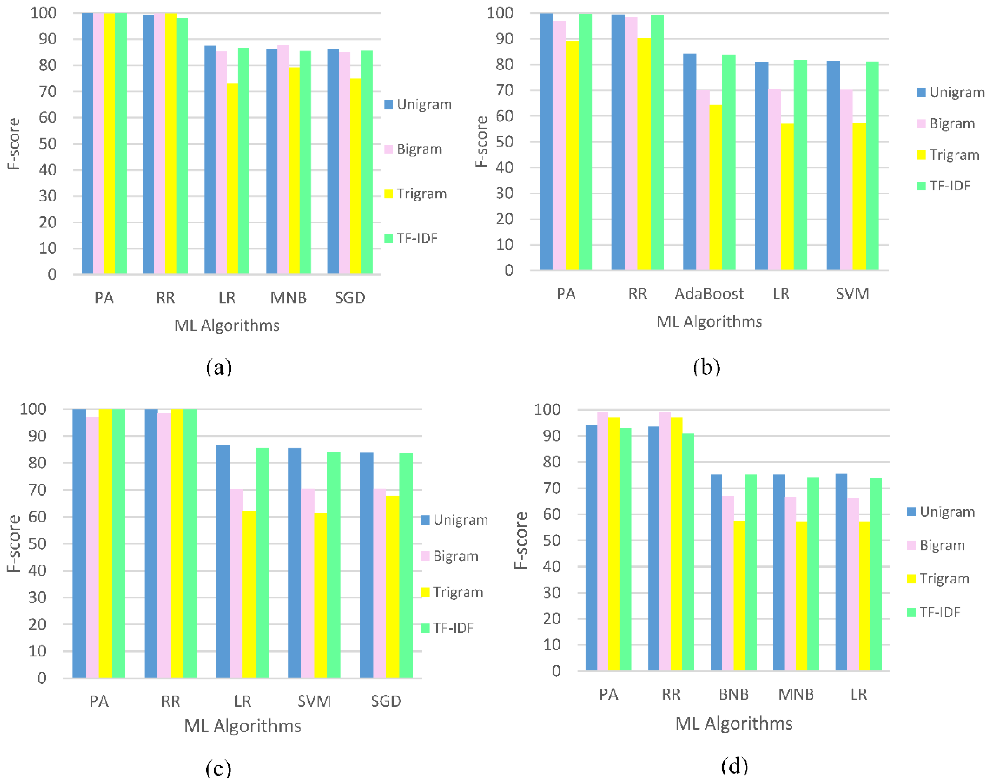
5. Results and Discussion

The comparative analysis of results obtained by the proposed methodology using four different datasets, n-gram and TF–IDF as FE is demonstrated in

Table 2. The comparison of various machine learning (ML) classifiers’ performance using different features.

ML Classifier	Dataset	IMDB				Cornell Movies				Amazon				Twitter
	Feature Extraction	Unigram	Bigram	Trigram	TF-IDF	Unigram	Bigram	Trigram	TF-IDF	Unigram	Bigram	Trigram	TF-IDF	Unigram	Bigram	Trigram	TF-IDF
NB	Acc.	85.76	87.56	79.16	65.56	69.76	60.76	70.36	52.46	79.66	58.66	50.56	67.06	74.66	65.96	53.76	70.16
	Prc.	85.96	87.56	79.16	65.96	78.56	70.76	70.36	52.16	79.66	67.36	64.66	67.66	74.86	66.46	60.96	70.36
	Rcl.	85.76	87.56	79.16	65.56	69.76	62.36	70.26	52.16	79.66	60.76	52.26	66.96	74.66	65.96	54.16	70.16
	F-S	85.86	87.56	79.16	65.76	73.86	66.26	70.36	52.16	79.66	63.86	57.86	67.36	74.76	66.26	57.36	70.26
BNB	Acc.	86.16	83.66	62.56	84.86	78.46	61.46	50.26	79.56	79.46	62.46	50.26	80.26	75.26	66.46	53.96	75.36
	Prc.	85.06	85.56	76.86	85.16	79.86	73.66	45.06	81.16	79.46	71.06	64.66	80.66	75.26	67.36	61.66	75.36
	Rcl.	84.76	83.66	62.66	84.86	78.46	62.86	50.16	79.56	79.66	63.76	51.76	80.36	75.26	66.46	53.96	75.36
	F-S	84.86	84.56	68.96	84.96	79.16	67.86	47.46	80.36	79.56	67.16	57.56	80.56	75.26	66.86	57.56	75.36
MNB	Acc.	86.16	87.56	79.06	85.46	82.06	62.26	70.26	81.66	79.46	59.66	50.56	79.06	75.26	66.26	53.76	74.26
	Prc.	86.26	87.56	79.26	85.46	81.96	73.86	70.36	81.66	79.56	68.06	64.66	79.56	75.36	66.86	60.86	74.26
	Rcl.	86.16	87.56	79.16	85.46	82.06	63.96	70.26	81.66	79.46	61.76	52.26	79.16	75.26	66.26	54.16	74.26
	F-S	86.26	87.66	79.16	85.46	82.06	68.56	70.36	81.66	79.56	64.76	57.86	79.36	75.36	66.56	57.26	74.26
AdaBoost	Acc.	80.36	65.26	57.96	80.46	83.06	64.06	57.96	84.46	83.56	63.76	55.76	83.26	64.46	52.76	51.16	64.46
	Prc.	80.56	72.86	68.26	80.56	83.06	77.86	74.16	84.46	84.96	77.76	76.46	84.66	64.66	67.86	62.66	69.66
	Rcl.	80.36	65.26	57.96	80.36	83.06	64.06	57.96	84.46	83.56	63.96	55.76	83.26	64.46	52.76	51.16	64.46
	F-S	80.46	68.76	62.76	80.46	83.06	70.36	65.06	84.46	84.26	70.16	64.46	83.96	66.96	59.36	56.36	66.96
ME	Acc.	85.66	87.16	78.56	64.36	68.16	57.96	69.56	52.36	77.26	56.76	51.66	64.86	74.76	65.96	53.86	70.46
	Prc.	85.86	87.26	78.56	64.86	77.76	70.06	69.76	52.36	77.86	67.76	64.16	67.46	74.96	66.56	61.36	70.56
	Rcl.	85.66	87.16	78.56	64.36	68.56	58.06	69.56	52.36	77.26	56.76	51.66	64.86	74.76	65.96	53.86	70.46
	F-S	85.76	87.26	78.56	64.56	72.86	63.46	69.66	52.36	77.56	61.76	57.26	66.16	74.86	66.26	57.36	70.46
SGD	Acc.	86.16	84.96	74.26	85.56	83.66	67.06	67.86	83.46	79.36	67.26	51.36	78.86	74.96	65.66	52.96	73.16
	Prc.	86.16	84.96	75.66	85.66	83.76	74.06	67.96	83.56	79.26	74.36	64.06	79.06	75.16	66.46	63.26	73.16
	Rcl.	86.16	84.96	74.26	85.56	83.76	67.16	67.86	83.46	79.16	67.56	51.56	78.76	74.96	65.66	52.96	73.16
	F-S	86.16	84.96	74.96	85.66	83.76	70.46	67.86	83.56	79.26	70.76	57.16	78.96	75.06	66.06	57.66	73.16
SVM	Acc.	85.76	85.26	73.36	84.56	85.56	67.26	53.56	84.16	81.36	66.76	51.66	81.16	73.66	64.86	53.86	71.46
	Prc.	85.76	85.26	74.36	84.56	85.56	74.06	72.36	84.16	81.36	73.76	64.16	81.36	73.66	65.36	60.96	71.46
	Rcl.	85.76	85.26	73.26	84.56	85.56	67.36	53.56	84.16	81.56	67.06	51.66	81.06	73.66	64.86	53.86	71.46
	F-S	85.76	85.26	73.86	84.56	85.56	70.56	61.56	84.16	81.46	70.26	57.26	81.26	73.66	65.16	57.16	71.46
LR	Acc.	87.46	85.26	72.16	86.56	86.46	67.46	55.36	85.66	80.86	67.66	51.46	81.56	75.56	65.86	53.96	74.06
	Prc.	87.56	85.36	73.66	86.56	86.46	72.96	71.06	85.66	81.16	73.16	64.06	81.76	75.56	66.46	61.06	74.06
	Rcl.	87.46	85.26	72.16	86.56	86.46	67.56	55.46	85.66	81.06	67.96	51.66	81.56	75.56	65.86	53.96	74.06
	F-S	87.56	85.36	72.96	86.56	86.46	70.16	62.26	85.66	81.06	70.46	57.16	81.66	75.56	66.16	57.26	74.06
PA	Acc.	99.96	99.86	99.86	99.96	99.96	96.76	99.96	99.96	99.86	96.76	87.76	99.76	94.16	99.26	96.86	92.96
	Prc.	99.96	99.86	99.86	99.96	99.96	96.96	99.96	99.96	99.76	96.96	90.26	99.76	94.16	99.26	97.06	92.96
	Rcl.	99.96	99.86	99.86	99.96	99.96	96.86	99.96	99.96	99.86	96.86	87.76	99.76	94.16	99.26	96.86	92.96
	F-S	99.96	99.86	99.86	99.96	99.96	96.96	99.96	99.96	99.86	96.86	88.96	99.76	94.16	99.26	96.96	92.96
RR	Acc.	99.16	99.86	99.86	98.26	99.96	98.46	99.96	99.96	99.36	98.46	89.26	99.06	93.46	99.16	96.86	90.86
	Prc.	99.16	99.86	99.86	98.26	99.96	98.56	99.96	99.96	99.36	98.46	91.16	99.06	93.46	99.16	97.06	90.96
	Rcl.	99.16	99.86	99.86	98.26	99.96	98.46	99.96	99.96	99.36	98.46	89.36	99.06	93.46	99.16	96.86	90.86
	F-S	99.16	99.86	99.86	98.26	99.96	98.46	99.96	99.96	99.36	98.46	90.26	99.06	93.46	99.16	96.96	90.96

.

From the experiments illustrated in Table 2, we recognized that the FE methods had an impact on the performance of any classifier. PA and RR with unigram, bigram or TF–IDF outperformed other algorithms on different datasets with an accuracy above 96%.

The top five accuracies of the results obtained by the proposed methodology using four different datasets, n-gram and TF–IDF as FE algorithms is demonstrated in Figure 3.

Seen in Figure 3, the top accuracies for the for IMDB dataset were for PA, RR, LR, NB and MNB. We noticed that the bigram performed the best with all ML algorithms, however, the unigram also received high accuracies. The trigram did not work very well with the IMDB dataset. In the Amazon products dataset we noticed that PA, RR, SVM, AdaBoost and LR achieved the highest accuracies. Using unigram or TF–IDF gave an accuracy above 80%, while trigram was the worst. The highest accuracies on Cornell movies dataset were for PA, RR, LR, SVM, and AdaBoost. Unigram and TF–IDF outperform the other FE methods. Trigram gave the lowest accuracies with most of ML algorithms. In the Twitter dataset, PA, RR, BNB, LR, and MNB achieved the highest accuracies. The trigram achieved the lowest accuracies among the different ML algorithms.

The top five precisions of the results obtained by the proposed methodology using four different datasets, n-gram and TF–IDF as FE algorithms is demonstrated in Figure 4.

Seen in Figure 4, the top precisions for the IMDB dataset were for PA, RR, LR, MNB, and ME. We noticed that the bigram performed the best with all ML algorithms, however, unigram also had a high precision. On Amazon products dataset we noticed that PA, RR, AdaBoost, SVM, and LR achieved the highest precision with using unigram or TF–IDF as FE methods. The highest precision values on Cornell movies dataset were for PA, RR, AdaBoost, LR, and SVM. Unigram and TF–IDF outperformed the other FE methods. On the Twitter Dataset, PA, RR, BNB, MNB, and LR achieved the highest precision. Trigram achieved the lowest precision among the different ML algorithms.

The top five show the results obtained by the proposed methodology using four different datasets, n-gram and TF–IDF as FE algorithms, this is demonstrated in Figure 5.

As seen in Figure 5 the top recall values for the IMDB dataset were for PA, RR, NB, LR and MNB. We noticed that n-gram beat the TF-IDF performance with all ML algorithms. On Amazon products dataset we noticed that PA, RR, AdaBoost, LR, and SVM achieved the highest recall values with using Unigram or TF-IDF as FE methods. The highest recall values on Cornell movies dataset were for PA, RR, LR, SVM, and SGD. Unigram and TF-IDF outperformed the other FE methods. On the Twitter dataset, PA, RR, BNB, MNB, and LR achieved the highest recall. Trigram achieved the lowest recall over different ML algorithms.

The top five f-score of the results obtained by the proposed methodology using four different datasets, n-gram and TF-IDF as FE algorithms is demonstrated in Figure 6.

As seen in Figure 6, the top f-score values for the IMDB dataset were for PA, RR, LR, MNB and SGD. We noticed that unigram, bigram and TF-IDF performed better than trigram. On the Amazon products dataset we noticed that PA, RR, AdaBoost, LR, and SVM achieved the highest f-score with using unigram or T-IDF as FE methods. The highest f-score values on Cornell movies dataset were for PA, RR, LR, SVM, and SGD. Unigram and TF–IDF outperformed the other FE methods. On the Twitter dataset, PA, RR, BNB, MNB, and LR achieved the highest f-score. Trigram achieved the lowest f-score among the different ML algorithms.

6. Conclusions and Future Work

In this research, ten different ML algorithms—NB, SGD, SVM, PA, ME, AdaBoost, MNB, BNB, RR and LR with two FE algorithms (n-gram and TF–IDF)—have been implemented on four SA datasets. The four reviews datasets are IMDB, Cornell movies, Amazon and Twitter, which have a different number of reviews each. The performance of the PA and RR with different FE algorithms on various datasets is the best among other algorithms as they give the highest accuracies in a range between 87% and 99.96%. Of the other tested algorithms, LR and SVM also promise an acceptable and convenient performance.

Some of the difficulties of sentiment analysis could be utilized as further extensions in the future of this research. The future research will focus on the detection of sarcasm and applying sentiment analysis to more domains such as YouTube, Yelp, Facebook, and cross-domains.

References

1. Gamal, D.; Alfonse, M.; El-Horbaty, E.S.; Salem, A.B. A comparative study on opinion mining algorithms of social media statuses. In Proceedings of the Intelligent Computing and Information Systems (ICICIS), Cairo, Egypt, 5–7 December 2017; pp. 385–390. [Google Scholar]
2. Petz, G.; Karpowicz, M.; Fürschuß, H.; Auinger, A.; Stříteský, V.; Holzinger, A. Opinion mining on the web 2.0—Characteristics of user generated content and their impacts. In Lecture Notes in Computer Science LNCS 7947; Springer: Berlin/Heidelberg, Germany, 2013; pp. 35–46. [Google Scholar] [CrossRef]
3. Zhang, Z.; Ye, Q.; Zhang, Z.; Li, Y. Sentiment classification of Internet resturant reviews written in Catonese. Expert Syst. Appl. 2011, 38, 7674–7682. [Google Scholar] [CrossRef]
4. Petz, G.; Karpowicz, M.; Fürschuß, H.; Auinger, A.; Stříteský, V.; Holzinger, A. Computational approaches for mining user’s opinions on the web 2.0. Inf. Process. Manag. 2015, 51, 510–519. [Google Scholar] [CrossRef]
5. Tripathy, A.; Agrawal, A.; Rath, S.K. Classification of sentiment reviews using n-gram machine learning approach. Expert Syst. Appl. 2016, 57, 117–126. [Google Scholar] [CrossRef]
6. Khoo, C.S.; Johnkhan, S.B. Lexicon-based sentiment analysis: Comparative evaluation of six sentiment lexicons. J. Inf. Sci. 2018, 44, 491–511. [Google Scholar] [CrossRef]
7. Dey, L.; Haque, S.M. Opinion mining from noisy text data. Int. J. Doc. Anal. Recognit. IJDAR 2009, 12, 205–226. [Google Scholar] [CrossRef]
8. Bouazizi, M.; Ohtsuki, T. Sentiment analysis: From binary to multi-class classification: A pattern-based approach for multi-class sentiment analysis in Twitter. In Proceedings of the IEEE International Conference Communications (ICC), Kuala Lumpur, Malaysia, 22–27 May 2016; pp. 1–6. [Google Scholar]
9. Barnaghi, P.; Ghaffari, P.; Breslin, J.G. Opinion mining and sentiment polarity on twitter and correlation between events and sentiment. In Proceedings of the Second international Conference Big Data Computing Service and Applications (BigDataService), Oxford, UK, 29 March–1 April 2016; pp. 52–57. [Google Scholar]
10. Liu, S.M.; Chen, J.-H. A multi-label classification based approach for sentiment classification. Int. J. Expert Syst. Appl. 2015, 42, 1083–1093. [Google Scholar] [CrossRef]
11. Joshi, N.S.; Itkat, S.A. A survey on feature level sentiment analysis. Int. J. Comput. Sci. Inf. Technol. 2014, 5, 5422–5425. [Google Scholar]
12. Deng, Z.-H.; Luo, K.-H.; Yu, H.-L. A study of supervised term weighting scheme for sentiment analysis. Expert Syst. Appl. 2014, 41, 3506–3513. [Google Scholar] [CrossRef]
13. Hima, S.; Gladston, R.S. Analysis of machine learning techniques for opinion mining. Int. J. Adv. Res. 2015, 3, 375–381. [Google Scholar]
14. Joshi, V.C.; Vekariya, V.M. An approach to sentiment analysis on Gujarati tweets. Int. J. Adv. Comput. Sci. Technol. 2017, 10, 1487–1493. [Google Scholar]
15. Liu, B. Sentiment analysis and subjectivity. Int. J. Handb. Nat. Lang. Process. 2010, 2, 627–666. [Google Scholar]
16. Wawre, S.V.; Deshmukh, S.N. Sentiment classification using machine learning algorithms. Int. J. Sci. Res. IJSR 2016, 5, 1–3. [Google Scholar]
17. Maas, A.L.; Daly, R.E.; Pham, P.T.; Huang, D.; Ng, A.Y.; Potts, C. Learning word vectors for sentiment analysis. In Proceedings of the 49th Annual Meeting of the Association for Computational Linguistics: Human Language Technologies, Portland, OR, USA, 19–24 June 2011. [Google Scholar]
18. Movie Review Data. Available online: http://www.cs.cornell.edu/people/pabo/movie-review-data/ (accessed on 2 August 2018).
19. Kotzias, D.; Denil, M.; de Freitas, N.; Smyth, P. From group to individual labels using deep features. In Proceedings of the 21th ACM SIGKDD International Conference on Knowledge Discovery and Data Mining, Sydney, Australia, 10–13 August 2015; pp. 597–606. [Google Scholar]
20. Twitter Sentiment Analysis Training Corpus (Dataset). Available online: http://thinknook.com/twitter-sentiment-analysis-training-corpus-dataset-2012-09-22/ (accessed on 2 August 2018).
21. The MIT License (MIT). Available online: http://vineetdhanawat.mit-license.org/ (accessed on 2 August 2018).
22. Pang, B.; Lee, L.; Vaithyanathan, S. Thumbs up? Sentiment classification using machine learning techniques. In Proceedings of the Association for Computational Linguistics (ACL)-02 Conference on Empirical Methods in Natural Language Processing, Stroudsburg, PA, USA, 6–7 July 2002; Volume 10, pp. 79–86. [Google Scholar]
23. Pang, B.; Lee, L. A sentimental education: Sentiment analysis using subjectivity summarization based on minimum cuts. In Proceedings of the 42nd Annual Meeting on Association for Computational Linguistics, Barcelona, Spain, 21–26 July 2004. [Google Scholar]
24. Derczynski, L.; Maynard, D.; Aswani, N.; Bontcheva, K. Microblog-genre noise and impact on semantic annotation accuracy. In Proceedings of the 24th ACM Conference on Hypertext and Social Media, Paris, France, 1–3 May 2013; ACM: New York, NY, USA, 2013; pp. 21–30. [Google Scholar] [Green Version]
25. Petz, G.; Karpowicz, M.; Fürschuß, H.; Auinger, A.; Winkler, S.M.; Schaller, S.; Holzinger, A. On text preprocessing for opinion mining outside of laboratory environments. In Active Media Technology, Lecture Notes in Computer Science, LNCS 7669; Huang, R., Ghorbani, A., Pasi, G., Yamaguchi, T., Yen, N., Jin, B., Eds.; Springer: Berlin/Heidelberg, Germany, 2012; pp. 618–629. [Google Scholar] [CrossRef]
26. Derczynski, L.; Ritter, A.; Clark, S.; Bontcheva, K. Twitter part-of-speech tagging for all: Overcoming sparse and noisy data. In Proceedings of the International Conference Recent Advances in Natural Language Processing RANLP 2013, Hissar, Bulgaria, 7–13 September 2013; pp. 198–206. [Google Scholar]
27. O’Keefe, T.; Koprinska, I. Feature selection and weighting methods in sentiment analysis. In Proceedings of the 14th Australasian Document Computing Symposium, Sydney, Australia, 4 December 2009. [Google Scholar]
28. Tamilselvi, A.; ParveenTaj, M. Sentiment analysis of micro blogs using opinion mining classification algorithm. Int. J. Sci. Res. IJSR 2013, 2, 196–202. [Google Scholar]
29. Kao, A.; Poteet, S.R. (Eds.) Natural Language Processing and Text Mining; Springer: Berlin/Heidelberg, Germany, 2007. [Google Scholar]
30. Aggarwal, C.C.; Zhai, C. (Eds.) Mining Text Data; Springer: Berlin/Heidelberg, Germany, 2012. [Google Scholar]
31. Srivastava, A.N.; Sahami, M. Text Mining: Classification, Clustering, and Applications; (Chapman and Hall/CRC): The CRC Press: Boca Raton, FL, USA, 2009. [Google Scholar]
32. Scikit-Learn Machine Learning in Python. Available online: https://scikit-learn.org/ (accessed on 17 July 2018).
33. Natural Language Toolkit. Available online: https://www.nltk.org/ (accessed on 17 July 2018).
34. Wan, Y.; Gao, Q. An ensemble sentiment classification system of twitter data for airline services analysis. In Proceedings of the International Conference on Data Mining Workshops (ICDMW), Atlantic City, NJ, USA, 14–17 November 2015; pp. 1318–1325. [Google Scholar]
Figure 1. The proposed methodology.
Make 01 00014 g001
Figure 2. The confusion matrix.
Make 01 00014 g002
Figure 3. Top five accuracies on different datasets: (a) IMDB (b) Amazon (c) Cornell Movies (d) Twitter.
Make 01 00014 g003
Figure 4. Top five precision on different datasets: (a) IMDB (b) Amazon (c) Cornell Movies (d) Twitter.
Make 01 00014 g004
Figure 5. Top Five Recall on Different Datasets: (a) IMDB (b) Amazon (c) Cornell Movies (d) Twitter.
Make 01 00014 g005
Figure 6. Top five F-score on different datasets: (a) IMDB (b) Amazon (c) Cornell Movies (d) Twitter.
Make 01 00014 g006