Using Collocation with Radial Basis Functions in a Pseudospectral Framework for a New Layerwise Shallow Shell Theory

Abstract

This work presents radial basis function collocation methods in pseudospectral form for forecasting the static deformations and free vibration characteristics of thin and thick cross-ply laminated shells. This method utilizes an innovative layerwise shallow shell theory that integrates both translational and rotational degrees of freedom. A collection of numerical examples illustrates the precision and efficacy of the suggested numerical method, highlighting its capability in resolving static and vibrational issues.

1. Introduction

The majority of numerical techniques for laminated shell analysis rely on finite element or analytical solutions. A accurate numerical technique and the suitable application of a shear deformation theory are necessary for an effective analysis. Shear deformation theories can be broadly divided into two groups: layerwise (LW) theories, in which each layer has distinct degrees of freedom, and equivalent single layer (ESL) theories, in which all layers share the same set of degrees of freedom. ESL theories are further subdivided into higher-order theories as in Pandya and Kant [1], Reddy and Liu [2], and Touratier [3], and first-order theories as the Mindlin’s plate theory [4]. LW theories can concentrate just on translational motion at each layer’s interfaces [5]. Carrera [6,7,8] developed a unified formulation that modifies the expansion vector for a particular plate/shell theory, allowing for the application of many theories.

Recently, the Kansa technique for collocation with radial basis functions (RBFs) have been presented (Kansa [9], Ferreira [10,11]). RBFs were first used to interpolate geographically scattered data by Hardy [12,13]. Later, they were utilized to solve partial differential equations (PDEs) by Kansa [9,14]. Using various shear deformation theories several successful applications of the RBF collocation to plates and shell were presented in [15,16]. A successful concurrent strong-form element method was given in [17]. Layerwise theories have undergone recent developments, as detailed in [18,19].

In this work, we employ an optimized shape parameter in conjunction with radial basis functions (RBFs) within a pseudospectral framework and a layerwise shell theory. We are able to investigate laminated shallow shell free vibrations and static deformations with this technology. The calculated values, which were attained by applying several techniques, are in very good agreement with the ones found in the literature.

2. Collocation with Radial Basis Functions in Pseudospectral Framework

Formulation

Pseudospectral (PS) methods [20,21] are able to deliver highly accurate approximate solutions to problems with partial differential equations (PDEs). In these methods, the spatial component $\widehat{u}$ of the approximate solution is represented as a linear combination of basis functions ${\varphi }_j$, where $j=1,\dots ,N$, as

$$\widehat{u}\left(x\right)=\sum _{j=1}^N{c}_j{\varphi }_j\left(x\right),x\in \mathbb{R}.$$

(1)

The utilization of polynomial basis functions in higher-dimensional spaces is generally confined to tensor products of one-dimensional basis functions. To overcome this issue, we substitute polynomials with radial basis functions (RBFs), enabling the modeling of uneven, general geometry grids with accuracy comparable to classic PS approaches.

In the realm of resolving linear partial differential equations, the radial basis function collocation approach, also known as Kansa’s method [9], necessitates that both the partial differential equation and the corresponding boundary conditions are fulfilled at a designated set of collocation locations, yielding a system of linear algebraic equations, that is solved to obtain coefficients $c_j$ in Equation  (1). The approximate solution $\widehat{u}$ can be computed then at any position x utilizing Equation (1).

Consider an elliptic PDE:

$$\mathcal{L}u=f\mathrm{in}\Omega ,$$

(2)

subject to Dirichlet boundary condition:

$$u=g\mathrm{on}\Gamma =\partial \Omega .$$

(3)

In the RBF-PS methodology, the solution is described as follows:

$$\widehat{u}\left({\displaystyle \mathit{x}}\right)=\sum _{j=1}^N{c}_j\phi (\parallel {\displaystyle \mathit{x}}-{{\displaystyle \mathit{\xi }}}_j\parallel ),{\displaystyle \mathit{x}}\in \Omega \subseteq {\mathrm{I}\mathrm{R}}^s,$$

(4)

where the points ${\mathit{\xi }}_j,j=1,\dots ,N$, serve as the centers of the RBF, with ${\varphi }_j=\phi \left(∥·-{\mathit{\xi }}_j∥\right)$. By evaluating Equation (4) at a set of collocation points ${\mathit{x}}_i,i=1,\dots ,N$, we obtain:

$$\widehat{u}\left(x_i\right)=\sum _{j=1}^N{c}_j\phi \left(∥x_i-{\xi }_j∥\right),i=1,\dots ,N$$

or in matrix-vector notation as:

$${\displaystyle \mathit{u}}=A{\displaystyle \mathit{c}},$$

(5)

where $\mathit{c}={\left[c_1,\dots ,c_N\right]}^T$ denotes the coefficient vector, and $A_{ij}=\phi \left(∥{\mathit{x}}_i-{\mathit{\xi }}_j∥\right)$ represents the matrix of RBF evaluations, and $\mathit{u}={\left[\widehat{u}\left({\mathit{x}}_1\right),\dots ,\widehat{u}\left({\mathit{x}}_N\right)\right]}^T$ denotes the vector of approximate solutions at the collocation sites.

A prevalent approach to executing the PS technique entails the formulation of a differentiation matrix $\mathbf{L}$, such that, at each grid point $x_i$, the relationship

$${\mathbf{u}}_{\mathcal{L}}=\mathbf{Lu}$$

(6)

is maintained, where ${\mathbf{u}}_{\mathcal{L}}$ denotes the vector of differentiated solution values.

The vector $\mathbf{u}={\left[\widehat{u}\left({\mathit{x}}_1\right),\dots ,\widehat{u}\left({\mathit{x}}_N\right)\right]}^T$ denotes the values of $\widehat{u}$ at the grid points, while ${\mathbf{u}}_{\mathcal{L}}$ indicates the vector of derivative values of u at the same locations. Instead of determining the coefficients c by solving a system of linear equations, as is standard in the conventional RBF collocation approach (Kansa’s method), we utilize the differentiation matrix $\mathbf{L}$. This yields a discrete formulation of the PDE as:

$$\mathbf{L}u=f,$$

(7)

where u is defined as previously stated, and f is the vector comprising the values of the right-hand side function f from Equation (2) assessed at the collocation points. In the differential Equation (2), the differential operator $\mathcal{L}$ is applied to the approximate solution $\widehat{u}$ as specified in Equation (4). According to linearity, we obtain:

$$\mathcal{L}\widehat{u}\left(\mathit{x}\right)=\sum _{j=1}^N{c}_j\mathcal{L}\phi \left(∥x-{\mathit{\xi }}_j∥\right)$$

Assessing this statement at the collocation sites $x_i$ yields a system of linear algebraic equations, which can be expressed in matrix-vector notation as:

$$\mathbf{L}u={\mathbf{A}}_{\mathcal{L}}\mathit{c}$$

(8)

where $\mathit{u}$ and $\mathit{c}$ are as defined in Equation (5), and the matrix $A_{\mathcal{L}}$ has entries ${\left.\mathcal{L}\phi \left(∥x-{\xi }_j∥\right)\right|}_{x=x_i}$. Although we do not explicitly calculate the coefficients $\mathit{c}$, they are given by $\mathit{c}=A^{-1}\mathit{u}$. Substituting this into the equation above, we obtain:

$$\mathbf{L}\mathit{u}={\mathbf{A}}_{\mathcal{L}}{\mathbf{A}}^{-1}\mathit{u}$$

(9)

The differentiation matrix $\mathbf{L}$ is defined as $\mathbf{L}={\mathbf{A}}_{\mathcal{L}}{\mathbf{A}}^{-1}$. To implement the Dirichlet boundary conditions from Equation (3), we substitute the rows of L associated with the boundary collocation points with conventional unit vectors, featuring a one in the diagonal position and zeros in all other positions. Furthermore, we substitute the equivalent values of $\mathbf{f}\left({\mathit{x}}_k\right)$ on the right-hand side with $g\left(x_k\right)$.

The shape parameter $\epsilon$ is essential in determining the precision of the numerical solution. The ideal value of $\epsilon$ is ascertained by Rippa’s [22] method, a form of cross-validation referred to as “leave-one-out” cross-validation (LOOCV). Despite the computational expense associated with a direct implementation of the LOOCV algorithm, Rippa shown that it may be streamlined into a singular formula:

$$E_k={\displaystyle \frac{c_k}{{\mathbf{A}}_{kk}^{-1}}},$$

(10)

where $c_k$ is the k th coefficient in the interpolant based on the full dataset, and ${\mathbf{A}}_{kk}^{-1}$ is the k th diagonal element of the inverse of the corresponding interpolation matrix.

We will now demonstrate the calculation of differentiation matrices utilizing three pseudospectral approaches. The initial approach utilizes Trefethen’s ‘cheb.m’ code as detailed in [21]. The last two approaches employ collocation with radial basis functions in a pseudospectral framework, utilizing differentiation matrices of size $(N+1)\times (N+1)$, where N denotes the number of nodes in the domain, inclusive of the boundaries. Such matrices facilitate the interpolation of the equations of motion, permitting resolution as a linear system of equations (in static scenarios) or as a generalized eigenvalue problem (in cases of free vibrations or buckling). Utilizing Trefethen’s ‘cheb.m’ code from [21], we derive the differentiation matrices in a concise format, as demonstrated in Program 1.

Program 1. 

Using cheb.m from Trefethen’s book [21]

% PS methd using Trefethen’s cheb.m code

[D,x] = cheb(N);

D2 = D^2;Dy=kron(D,I);

Dx=kron(I,D);

Dxx=kron(I,D2);

Dyy=kron(D2,I);

Dxy=Dx{*}Dy;

In the context of employing radial basis functions in a univariate framework, we initially calculate the differentiation matrix D. Thereafter, we derive the differentiation matrices ${\mathbf{D}}_x,{\mathbf{D}}_{xx}$, and others by employing the Kronecker product through MATLAB’s (2024 version) kron function, as demonstrated in Program 2. The shape parameter epsilon is calculated via Rippa’s algorithm, as detailed by Ferreira and Fasshauer in [23].

Program 2. 

Using RBFs in tensor-product mode

% Kansa’s unsymmetric method on tensor-product grids

rbf = @(e,r) exp(-(e*r).^2);

drbf = @(e,r,dx) -2*e^2*dx.*exp(-(e*r).^2);

d2rbf = @(e,r) 2*e^2*(2*(e*r).^2-1).*exp(-(e*r).^2);

r = DistanceMatrix(x,x);

dx = DifferenceMatrix(x,x);

maxepsilon = 5;minepsilon = .1;

[epsilon,fval,exitflag,output] = fminbnd(@(epsilon)...

CostEpsilonDxRBFPS(epsilon,r,dx),minepsilon,maxepsilon);

ep=epsilon;

A = rbf(ep,r);

DA = drbf(ep,r,dx);

D = DA/A;D2A = d2rbf(ep,r);

D2 = D2A/A;

Dy=kron(D,I);

Dx=kron(I,D);

Dxx=kron(I,D2);

Dyy=kron(D2,I);

Dxy=Dx{*}Dy;

The methodologies outlined in Programs 1 and 2 are confined to tensor-product grids, which may be constraining for specific engineering applications. This code calculates differentiation matrices for generic two-dimensional grids to overcome this constraint.

Program 3. 

Using RBFs in general 2D grids

% Kansa’s unsymmetric method on general grids

[Dx,x,y,epsilon] = DxRBF(N);

[Dy,x,y] = DyRBF(N,epsilon);

[Dxx,x,y] = DxxRBF(N,epsilon);

[Dxy,x,y] = DxyRBF(N,epsilon);

[Dyy,x,y] = DyyRBF(N,epsilon);

In Program 4, we illustrate the computation of the matrix $D_x$, which encompasses the first derivatives concerning x. Comparable procedures can be utilized to derive matrices for additional derivatives. In accordance with the methodology established by Ferreira and Fasshauer [23], we delineate the procedure for calculating the shape parameter epsilon utilizing Rippa’s algorithm in Program 5. It is essential to acknowledge that an other differentiation matrix may have been employed instead of $D_x$.

Program 4. 

Computing D_x

% DxRBF  compute D = differentiation matrix, x,y = Chebyshev grids

function [D,x,y,epsilon] = DxRBF(N,epsilon)

global rbf dxrbf dyrbf dxxrbf dxyrbf dyyrbf Lrbf L2rbf d2rbf

if N==0, D=0; x=1; return, end

x = cos(pi*(0:N)/N)’;   % Chebyshev points

y=x;[xx,yy] = meshgrid(x,y);

points = [xx(:) yy(:)];

r = DistanceMatrix(points,points);

dx = DifferenceMatrix(xx,xx);

if nargin == 1

% Shape parameter interval

maxepsilon = 10;

minepsilon = .1;

[epsilon,fval,exitflag,output] = fminbnd(@(epsilon) ...

CostEpsilonDxRBF(epsilon,r,dx),minepsilon,maxepsilon);

end

A = rbf(epsilon,r);

DA = dxrbf(epsilon,r,dx);

D = DA/A;

Program 5. 

Computing error for Rippa’s algorithm

% CostEpsilonDxRBF

function ceps = CostEpsilonDxRBF(epsilon,r,dx)

global rbf dxrbf

[m,n] = size(r);

A = rbf(epsilon,r);

rhs = dxrbf(epsilon,r,dx)’;

invA = pinv(A);

EF = (invA*rhs)./repmat(diag(invA),1,m);

ceps = norm(EF(:),2);

In this third RBF-PS approach, we generally employ the Wendland $C^6$ functions, as specified in Program 6. In this case, e signifies the shape parameter, r indicates the Euclidean distance between two grid points, and $dx$ refers to its first derivative concerning x, among others.

Program 6. 

Wendland C6 function and its derivatives

rbf = @(e,r) max(1-e*r,0).^8.*(32*(e*r).^3+25*(e*r).^2+8*e*r+1);

dxrbf = @(e,r,dx) -22*dx*e^2.*...

max(1-e*r,0).^7.*(16*(e*r).^2+7*e*r+1);

dyrbf = @(e,r,dy) -22*dy*e^2.*...

max(1-e*r,0).^7.*(16*(e*r).^2+7*e*r+1);

dxxrbf = @(e,r,dx) 22*e^2*max(1-e*r,0).^6.*...

(16*e^3*(r.^2+9*dx.^2).*r+3*e^2*(8*dx.^2-3*r.^2)-6*e*r-1);

dxyrbf = @(e,r,dx,dy) 528*e^4*dx.*dy.*...

max(1-e*r,0).^6.*(6*e*r+1);

dyyrbf = @(e,r,dy) 22*e^2*max(1-e*r,0).^6.*...

(16*e^3*(r.^2+9*dy.^2).*r+3*e^2*(8*dy.^2-3*r.^2)-6*e*r-1);

3. The Layerwise Theory

We introduce a simple and efficient layerwise shallow shell theory. A Mindlin shell is situated in the intermediate layer. Subsequently, we overlay an upper and a lower layer above and below the middle layer, guaranteeing that the displacements at the interfaces between the layers remain continuous. The lowest, medium, and highest levels are marked as 1, 2, and 3, accordingly.

3.1. Displacement Field

The displacement field encompasses nine degrees of freedom: three displacements $\left(u_0,v_0,w_0\right)$ of the mid-surface of the second layer, and six rotations $\left({\theta }_x\left(k\right),{\theta }_y\left(k\right),k=1,2,3\right)$ of the normal to the mid-plane of each respective layer about the y and x axes. For clarity, we designate the displacement field as layer 2, also referred to as the middle layer or sandwich core. This field is characterized by the subsequent equation:

$${(u,v,w)}^{\left(2\right)}=\left(u_0,v_0,w_0\right)+z^{\left(2\right)}\left({\theta }_x^{\left(2\right)},{\theta }_y^{\left(2\right)},0\right)$$

(11)

For layer 3, by imposing continuity of displacements at the layers 2–3, we obtain

$${(u,v,w)}^{\left(3\right)}=\left(u_0,v_0,w_0\right)+z^{\left(3\right)}\left({\theta }_x^{\left(3\right)},{\theta }_y^{\left(3\right)},0\right)+{\displaystyle \frac{h_2}{2}}\left({\theta }_x^{\left(2\right)},{\theta }_y^{\left(2\right)},0\right)+{\displaystyle \frac{h_3}{2}}\left({\theta }_x^{\left(3\right)},{\theta }_y^{\left(3\right)},0\right)$$

(12)

For layer 1 (lower layer or lower sandwich skin), by imposing continuity of displacements at the layers 1–2, we obtain

$${(u,v,w)}^{\left(1\right)}=\left(u_0,v_0,w_0\right)+z^{\left(1\right)}\left({\theta }_x^{\left(1\right)},{\theta }_y^{\left(1\right)},0\right)-{\displaystyle \frac{h_2}{2}}\left({\theta }_x^{\left(2\right)},{\theta }_y^{\left(2\right)},0\right)-{\displaystyle \frac{h_1}{2}}\left({\theta }_x^{\left(1\right)},{\theta }_y^{\left(1\right)},0\right)$$

(13)

In Equations (11)–(13), $h_k$ represents the thickness of layer k, and $z^{\left(k\right)}$ represents the z-coordinates for each layer k and is defined within the interval $z\in \left[-h_k/2,h_k/2\right]$.

3.2. Deformations

In this shallow shell theory, we regard x and y as curvilinear coordinates, with $R_x$ and $R_y$ representing the radii of curvature in the $xz$ and $yz$ planes, respectively. The in-plane deformations may be defined as:

$$\left\{\begin{array}{c}{\epsilon }_{xx}^{\left(k\right)}\\ {\epsilon }_{yy}^{\left(k\right)}\\ {\gamma }_{xy}^{\left(k\right)}\end{array}\right\}=\left\{\begin{array}{c}{\epsilon }_{xx}^m\\ {\epsilon }_{yy}^m\\ {\gamma }_{xy}^m\end{array}\right\}+z^{\left(k\right)}\left\{\begin{array}{c}{\epsilon }_{xx}^{f\left(k\right)}\\ {\epsilon }_{yy}^{f\left(k\right)}\\ {\gamma }_{xy}^{f\left(k\right)}\end{array}\right\}+\left\{\begin{array}{c}{\epsilon }_{xx}^{mf\left(k\right)}\\ {\epsilon }_{yy}^{mf\left(k\right)}\\ {\gamma }_{xy}^{mp}f\left(k\right)\end{array}\right\}+\left\{\begin{array}{c}{\epsilon }_{xx}^{w_0}\\ {\epsilon }_{yy}^{w_0}\\ {\gamma }_{xy}^{w_0}\end{array}\right\}$$

(14)

where the membrane constituents are the same throughout the three layers:

$${\left({\epsilon }_{xx},{\epsilon }_{yy},{\gamma }_{xy}\right)}^m=\left({\displaystyle \frac{\partial u_0}{\partial x}},{\displaystyle \frac{\partial v_0}{\partial y}},{\displaystyle \frac{\partial u_0}{\partial y}}+{\displaystyle \frac{\partial v_0}{\partial x}}\right)$$

(15)

For every layer k, the bending deformations are described as:

$${\left({\epsilon }_{xx},{\epsilon }_{yy},{\gamma }_{xy}\right)}^{f\left(k\right)}=\left({\displaystyle \frac{\partial {\theta }_x^{\left(k\right)}}{\partial x}},{\displaystyle \frac{\partial {\theta }_y^{\left(k\right)}}{\partial y}},{\displaystyle \frac{\partial {\theta }_x^{\left(k\right)}}{\partial y}}+{\displaystyle \frac{\partial {\theta }_y^{\left(k\right)}}{\partial x}}\right)$$

(16)

The deflection components related to the radius of curvatures are given by:

$$\left({\epsilon }_{x{x}_0}^{w_0},{\epsilon }_{yy}^{w_0},{\gamma }_{xy}^{w_0}\right\}=\left({\displaystyle \frac{w_0}{R_x}},{\displaystyle \frac{w_0}{R_y}},0\right)$$

(17)

The membrane-bending coupling components for layers 2, 3, and 1 are specified as follows:

$${\left({\epsilon }_{xx},{\epsilon }_{yy},{\gamma }_{xy}\right)}^{mf\left(2\right)}=(0,0,0)$$

(18)

$$\begin{array}{cc}\hfill & {\left({\epsilon }_{xx},{\epsilon }_{yy},{\gamma }_{xy}\right)}^{mf\left(3\right)}=\hfill \\ \hfill & \left({\displaystyle \frac{h_2}{2}}{\displaystyle \frac{\partial {\theta }_x^{\left(2\right)}}{\partial x}}+{\displaystyle \frac{h_3}{2}}{\displaystyle \frac{\partial {\theta }_x^{\left(3\right)}}{\partial x}},{\displaystyle \frac{h_2}{2}}{\displaystyle \frac{\partial {\theta }_y^{\left(2\right)}}{\partial y}}+{\displaystyle \frac{h_3}{2}}{\displaystyle \frac{\partial {\theta }_y^{\left(3\right)}}{\partial y}},{\displaystyle \frac{h_2}{2}}{\displaystyle \frac{\partial {\theta }_x^{\left(2\right)}}{\partial y}}+{\displaystyle \frac{h_3}{2}}{\displaystyle \frac{\partial {\theta }_x^{\left(3\right)}}{\partial y}}+{\displaystyle \frac{h_2}{2}}{\displaystyle \frac{\partial {\theta }_y^{\left(2\right)}}{\partial x}}+{\displaystyle \frac{h_3}{2}}{\displaystyle \frac{\partial {\theta }_y^{\left(3\right)}}{\partial x}}\right)\hfill \end{array}$$

(19)

$$\begin{array}{cc}\hfill & {\left({\epsilon }_{xx},{\epsilon }_{yy},{\gamma }_{xy}\right)}^{mf\left(1\right)}=\hfill \\ \hfill & -\left({\displaystyle \frac{h_2}{2}}{\displaystyle \frac{\partial {\theta }_x^{\left(2\right)}}{\partial x}}+{\displaystyle \frac{h_1}{2}}{\displaystyle \frac{\partial {\theta }_x^{\left(1\right)}}{\partial x}},{\displaystyle \frac{h_2}{2}}{\displaystyle \frac{\partial {\theta }_y^{\left(2\right)}}{\partial y}}+{\displaystyle \frac{h_1}{2}}{\displaystyle \frac{\partial {\theta }_y^{\left(1\right)}}{\partial y}},{\displaystyle \frac{h_2}{2}}{\displaystyle \frac{\partial {\theta }_x^{\left(2\right)}}{\partial y}}+{\displaystyle \frac{h_1}{2}}{\displaystyle \frac{\partial {\theta }_x^{\left(1\right)}}{\partial y}}+{\displaystyle \frac{h_2}{2}}{\displaystyle \frac{\partial {\theta }_y^{\left(2\right)}}{\partial x}}+{\displaystyle \frac{h_1}{2}}{\displaystyle \frac{\partial {\theta }_y^{\left(1\right)}}{\partial x}}\right)\hfill \end{array}$$

(20)

For each layer k, the transverse shear deformations are calculated as follows:

$${\left({\gamma }_{xz},{\gamma }_{yz}\right)}^{\left(k\right)}=\left({\theta }_x^{\left(k\right)}+{\displaystyle \frac{\partial w_0}{\partial x}}-{\displaystyle \frac{u_0}{R_x}},{\theta }_y^{\left(k\right)}+{\displaystyle \frac{\partial w_0}{\partial y}}-{\displaystyle \frac{v_0}{R_y}}\right)$$

(21)

3.3. Stresses

The current layerwise approach disregards transverse normal deformations by presuming a uniform transverse displacement across each layer. Disregarding ${\sigma }_{zz}$ for each orthotropic layer, the stress-strain relationships in the fiber’s local coordinate system can be described as:

$${\left[\begin{array}{c}{\sigma }_{11}\\ {\sigma }_{22}\\ {\tau }_{12}\\ {\tau }_{13}\\ {\tau }_{23}\end{array}\right]}^{\left(k\right)}={\left[\begin{array}{ccccc}{C}_{11}& C_{12}& 0& 0& 0\\ C_{12}& C_{22}& 0& 0& 0\\ 0& 0& C_{66}& 0& 0\\ 0& 0& 0& C_{55}& 0\\ 0& 0& 0& 0& C_{44}\end{array}\right]}^{\left(k\right)}·{\left[\begin{array}{c}{\epsilon }_{11}\\ {ϵ}_{22}\\ {\gamma }_{12}\\ {\gamma }_{13}\\ {\gamma }_{23}\end{array}\right]}^{\left(k\right)}$$

(22)

The material coefficients $C_{ij}^{\left(k\right)}$ are expressible in terms of the engineering constants, specifically the elastic coefficients $v_{12}^{\left(k\right)},E_1^{\left(k\right)},E_2^{\left(k\right)}$, and $G_{12}^{\left(k\right)}$:

$$\begin{array}{cc}\hfill & C_{11}^{\left(k\right)}={\displaystyle \frac{E_1\left(k\right)}{1-v_{12}\left(k\right)·v_{21}\left(k\right)}};C_{12}^{\left(k\right)}=C_{21}^{\left(k\right)}={v_{21}}^{\left(k\right)}·{C_{11}}^{\left(k\right)};{v_{21}}^{\left(k\right)}=v_{12}\left(k\right){\displaystyle \frac{E_2^{\left(k\right)}}{E_1^{\left(k\right)}}}\hfill \\ \hfill & C_{22}^{\left(k\right)}={\displaystyle \frac{E_2^{\left(k\right)}}{1-v_{12}^{\left(k\right)}·v_{21}\left(k\right)}};{C_{66}}^{\left(k\right)}={G_{12}}^{\left(k\right)};{C_{55}}^{\left(k\right)}={G_{13}}^{\left(k\right)};{C_{44}}^{\left(k\right)}={G_{23}}^{\left(k\right)}\hfill \end{array}$$

(23)

This theory does not necessitate the application of shear correction factors. The stress-strain relations for each layer in shell coordinates are derived using material coefficients transformation rules as outlined by [5]

$${\left[\begin{array}{c}{\sigma }_{xx}\\ {\sigma }_{yy}\\ {\tau }_{xy}\\ {\tau }_{xz}\\ {\tau }_{yz}\end{array}\right]}^{\left(k\right)}={\left[\begin{array}{ccccc}{\overline{C}}_{11}& {\overline{C}}_{12}& {\overline{C}}_{16}& 0& 0\\ {\overline{C}}_{12}& {\overline{C}}_{22}& {\overline{C}}_{26}& 0& 0\\ {\overline{C}}_{16}& {\overline{C}}_{26}& {\overline{C}}_{66}& 0& 0\\ 0& 0& 0& {\overline{C}}_{55}& {\overline{C}}_{45}\\ 0& 0& 0& {\overline{C}}_{45}& {\overline{C}}_{44}\end{array}\right]}^{\left(k\right)}·{\left[\begin{array}{c}{\epsilon }_{xx}\\ {ϵ}_{yy}\\ {\gamma }_{xy}\\ {\gamma }_{xz}\\ {\gamma }_{yz}\end{array}\right]}^{\left(k\right)}$$

(24)

4. Equations of Motion

We can get the equations of motion from the dynamic form of the principle of virtual displacements:

$$0={\int }_0^T(\delta U+\delta V-\delta K)dt$$

(25)

The virtual strain energy $\left(\delta U\right)$, the virtual work performed by applied forces $\left(\delta V\right)$, and the virtual kinetic energy $\left(\delta K\right)$ for a three-layer laminate are defined as follows:

$$\begin{array}{c}\delta U={\int }_{{\Omega }_0}\sum _{k=1}^3\left\{{\int }_{-h_k/2}^{h_k/2}\left[{\sigma }_{xx}^{\left(k\right)}·\delta {\epsilon }_{xx}^{\left(k\right)}+{\sigma }_{yy}^{\left(k\right)}·\delta {\epsilon }_{yy}^{\left(k\right)}+{\tau }_{xy}^{\left(k\right)}·\delta {\gamma }_{xy}^{\left(k\right)}+{\tau }_{xz}^{\left(k\right)}\delta {\gamma }_{yz}^{\left(k\right)}+{\tau }_{yz}^{\left(k\right)}\delta {\gamma }_{yz}^{\left(k\right)}\right]dz\right\}dxdy\end{array}$$

(26)

$$\begin{array}{c}\delta V=-{\int }_{{\Omega }_0}\left[q·\delta w_0\right]dxdy-{\int }_{{\Gamma }_{\sigma }}\sum _{k=1}^3\left\{{\int }_{-h_k/2}^{h_k/2}\left[{\widehat{\sigma }}_{nn}\delta u_n+{\widehat{\sigma }}_{ns}\delta u_s+{\widehat{\sigma }}_{nz}\delta w\right]\right\}dzds\end{array}$$

(27)

$$\begin{array}{c}\delta K={\int }_{{\Omega }_0}\sum _{k=1}^3\left\{{\int }_{-h_k/2}^{h_{k/2}}{\rho }^k\left[{\dot{u}}^{\left(k\right)}\delta {\dot{u}}^{\left(k\right)}+{\dot{v}}^{\left(k\right)}\delta {\dot{v}}^{\left(k\right)}+{\dot{w}}^{\left(k\right)}\delta {\dot{w}}^{\left(k\right)}\right]\right\}dzdxdy\end{array}$$

(28)

In this context, $\delta$ quantities are defined as virtual. The symbol ${\Omega }_0$ indicates the midplane of the laminate, while ${\Gamma }_{\sigma }$ signifies the natural boundary. The variable q represents the external distributed load. The notation $(·)$ is used to denote time differentiation, and ${\rho }^k$ refers to the density of the material for layer k.

The virtual strain energy $\left(\delta U\right)$ can now be expressed in terms of the stress resultants and bending moments as

$$\begin{array}{cc}\hfill \delta U={\int }_{{\Omega }_0}\sum _{k=1}^3& \left\{\left(N_{xx}^{\left(k\right)}·\delta {\epsilon }_{xx}^m+M_{xx}^{\left(k\right)}·\delta {\epsilon }_{xx}^{f\left(k\right)}+N_{xx}^{\left(k\right)}·\delta {\epsilon }_{xx}^{mf\left(k\right)}+N_{xx}^{\left(k\right)}·\delta {\epsilon }_{xx}^{w_0}\right)\right.\hfill \\ \hfill & +\left(N_{yy}^{\left(k\right)}·\delta {\epsilon }_{yy}^m+M_{yy}^{\left(k\right)}·\delta {\epsilon }_{yy}^{f\left(k\right)}+N_{yy}^{\left(k\right)}·\delta {\epsilon }_{yy}^{mf\left(k\right)}+N_{yy}^{\left(k\right)}·\delta {\epsilon }_{yy}^{w_0}\right)\hfill \\ \hfill & +\left(N_{xy}^{\left(k\right)}·\delta {\gamma }_{xy}^m+M_{xy}^{\left(k\right)}·\delta {\gamma }_{xy}^{f\left(k\right)}+N_{xy}^{\left(k\right)}·\delta {\gamma }_{xy}^{mf\left(k\right)}+N_{xy}^{\left(k\right)}·\delta {\gamma }_{xy}^{w_0}\right)\hfill \\ \hfill & \left.+Q_x^{\left(k\right)}·\delta {\gamma }_{xz}^{\left(k\right)}+Q_y^{\left(k\right)}·\delta {\gamma }_{yz}^{\left(k\right)}\right\}dxdy\hfill \end{array}$$

(29)

where the in-plane stress resultants and bending moments are defined as

$$\begin{array}{c}\left(N_{xx},N_{yy},N_{xy}\right)=\sum _{k=1}^3{\int }_{-\frac{h_k}{2}}^{\frac{h_k}{2}}{\left({\sigma }_{xx},{\sigma }_{yy},{\tau }_{xy}\right)}^{\left(k\right)}dz\end{array}$$

(30)

$$\begin{array}{c}\left(M_{xx},M_{yy},M_{xy}\right)=\sum _{k=1}^3{\int }_{-\frac{h_k}{2}}^{\frac{h_k}{2}}z{\left({\sigma }_{xx},{\sigma }_{yy},{\tau }_{xy}\right)}^{\left(k\right)}dz\end{array}$$

(31)

and where the out-of-plane stress resultants are defined as

$$\left(Q_x,Q_y\right)=\sum _{k=1}^3{\int }_{-\frac{h_k}{2}}^{\frac{h_k}{2}}{\left({\tau }_{xz},{\tau }_{yz}\right)}^{\left(k\right)}dz$$

(32)

The work done by the external applied forces is defined as

$$\delta V=-\int q·\delta w_{0}dxdy$$

(33)

whereas the virtual kinetic energy is defined as

$$\delta K={\int }_{{\Omega }_0}\sum _{k=1}^3\left\{{\int }_{-h_k/2}^{h_k/2}{\rho }^k\left[{\dot{u}}^{\left(k\right)}\delta {\dot{u}}^{\left(k\right)}+{\dot{v}}^{\left(k\right)}\delta {\dot{v}}^{\left(k\right)}+{\dot{w}}^{\left(k\right)}\delta {\dot{w}}^{\left(k\right)}\right]\right\}dzdxdy$$

(34)

By gathering the coefficients of each virtual displacement and applying integration by parts, the dynamic equilibrium equations are derived by equating the coefficients of $\left(\delta u_0,\delta v_0,\delta w_0,\left\{\delta {\theta }_x^{\left(k\right)},\delta {\theta }_y^{\left(k\right)},k=1,2,3\right\}\right)$ to zero individually over ${\Omega }_0$:

$$\begin{array}{cc}\hfill & \delta u_0:\sum _{k=1}^3\left({\displaystyle \frac{\partial N_{xx}^{\left(k\right)}}{\partial x}}+{\displaystyle \frac{\partial N_{xy}^{\left(k\right)}}{\partial y}}+{\displaystyle \frac{Q_x^{\left(k\right)}}{R_x}}\right)=I_0^{\left(1\right)}\left({\displaystyle \frac{{\partial }^2{u}_0}{\partial t^2}}-{\displaystyle \frac{h_2}{2}}{\displaystyle \frac{{\partial }^2{\theta }_x^{\left(2\right)}}{d{t}^2}}-{\displaystyle \frac{h_1}{2}}{\displaystyle \frac{{\partial }^2{\theta }_x^{\left(1\right)}}{d{t}^2}}\right)+\hfill \\ \hfill & I_0^{\left(2\right)}{\displaystyle \frac{{\partial }^2{u}_0}{\partial t^2}}+I_0^{\left(3\right)}\left({\displaystyle \frac{{\partial }^2{u}_0}{\partial t^2}}+{\displaystyle \frac{h_2}{2}}{\displaystyle \frac{{\partial }^2{\theta }_x^{\left(2\right)}}{d{t}^2}}+{\displaystyle \frac{h_3}{2}}{\displaystyle \frac{{\partial }^2{\theta }_x^{\left(3\right)}}{d{t}^2}}\right)\hfill \end{array}$$

(35)

$$\begin{array}{cc}\hfill & \delta v_0:\sum _{k=1}^3\left({\displaystyle \frac{\partial N_{yy}^{\left(k\right)}}{\partial y}}+{\displaystyle \frac{\partial N_{xy}^{\left(k\right)}}{\partial x}}+{\displaystyle \frac{Q_y^{\left(k\right)}}{R_y}}\right)=I_0^{\left(1\right)}\left({\displaystyle \frac{{\partial }^2{v}_0}{\partial t^2}}-{\displaystyle \frac{h_2}{2}}{\displaystyle \frac{{\partial }^2{\theta }_y^{\left(2\right)}}{d{t}^2}}-{\displaystyle \frac{h_1}{2}}{\displaystyle \frac{{\partial }^2{\theta }_y^{\left(1\right)}}{d{t}^2}}\right)+I_0^{\left(2\right)}{\displaystyle \frac{{\partial }^2{v}_0}{\partial t^2}}\hfill \\ \hfill & +I_0^{\left(3\right)}\left({\displaystyle \frac{{\partial }^2{v}_0}{\partial t^2}}+{\displaystyle \frac{h_2}{2}}{\displaystyle \frac{{\partial }^2{\theta }_y^{\left(2\right)}}{d{t}^2}}+{\displaystyle \frac{h_3}{2}}{\displaystyle \frac{{\partial }^2{\theta }_y^{\left(3\right)}}{d{t}^2}}\right)\hfill \end{array}$$

(36)

$$\begin{array}{c}\delta w_0:\sum _{k=1}^3\left(-{\displaystyle \frac{N_{xx}^{\left(k\right)}}{R_x}}-{\displaystyle \frac{N_{yy}^{\left(k\right)}}{R_y}}+{\displaystyle \frac{\partial Q_x^{\left(k\right)}}{\partial x}}+{\displaystyle \frac{\partial Q_y^{\left(k\right)}}{\partial y}}\right)+q=I_0^{\left(1\right)}{\displaystyle \frac{{\partial }^2{\omega }_0}{\partial t^2}}+I_0^{\left(2\right)}{\displaystyle \frac{{\partial }^2{\omega }_0}{\partial t^2}}+I_0^{\left(3\right)}{\displaystyle \frac{{\partial }^2{\omega }_0}{\partial t^2}}\end{array}$$

(37)

$$\begin{array}{c}\delta {\theta }_x^{\left(1\right)}:{\displaystyle \frac{\partial M_{xx}^{\left(1\right)}}{\partial x}}-{\displaystyle \frac{h_1}{2}}{\displaystyle \frac{\partial N_{xx}^{\left(1\right)}}{\partial x}}+{\displaystyle \frac{\partial M_{xy}^{\left(1\right)}}{\partial y}}-{\displaystyle \frac{h_1}{2}}{\displaystyle \frac{\partial N_{xy}^{\left(1\right)}}{\partial y}}-Q_x^{\left(1\right)}\\ =I_0^{\left(1\right)}\left(-{\displaystyle \frac{h_1}{2}}{\displaystyle \frac{{\partial }^2{u}_0}{d{t}^2}}+{\displaystyle \frac{h_1{h}_2}{4}}{\displaystyle \frac{{\partial }^2{\theta }_x^{\left(2\right)}}{d{t}^2}}+{\displaystyle \frac{h_1^2}{4}}{\displaystyle \frac{{\partial }^2{\theta }_x^{\left(1\right)}}{d{t}^2}}\right)+I_2^{\left(1\right)}{\displaystyle \frac{{\partial }^2{\theta }_x^{\left(1\right)}}{\partial t^2}}\end{array}$$

(38)

$$\begin{array}{c}\delta {\theta }_y^{\left(1\right)}:{\displaystyle \frac{\partial M_{yy}^{\left(1\right)}}{\partial y}}-{\displaystyle \frac{h_1}{2}}{\displaystyle \frac{\partial N_{yy}^{\left(1\right)}}{\partial y}}+{\displaystyle \frac{\partial M_{xy}^{\left(1\right)}}{\partial x}}-{\displaystyle \frac{h_1}{2}}{\displaystyle \frac{\partial N_{xy}^{\left(1\right)}}{\partial x}}-Q_y^{\left(1\right)}\\ =I_0^{\left(1\right)}\left(-{\displaystyle \frac{h_1}{2}}{\displaystyle \frac{{\partial }^2{v}_0}{d{t}^2}}+{\displaystyle \frac{h_1{h}_2}{4}}{\displaystyle \frac{{\partial }^2{\theta }_y^{\left(2\right)}}{d{t}^2}}+{\displaystyle \frac{h_1^2}{4}}{\displaystyle \frac{{\partial }^2{\theta }_y^{\left(1\right)}}{d{t}^2}}\right)+I_2^{\left(1\right)}{\displaystyle \frac{{\partial }^2{\theta }_y^{\left(1\right)}}{\partial t^2}}\end{array}$$

(39)

$$\begin{array}{c}\delta {\theta }_x^{\left(2\right)}:{\displaystyle \frac{\partial M_{xx}^{\left(2\right)}}{\partial x}}+{\displaystyle \frac{h_2}{2}}{\displaystyle \frac{\partial N_{xx}^{\left(3\right)}}{\partial x}}-{\displaystyle \frac{h_2}{2}}{\displaystyle \frac{\partial N_{xx}^{\left(1\right)}}{\partial x}}+{\displaystyle \frac{\partial M_{xy}^{\left(2\right)}}{\partial y}}+{\displaystyle \frac{h_2}{2}}{\displaystyle \frac{\partial N_{xy}^{\left(3\right)}}{\partial y}}-{\displaystyle \frac{h_2}{2}}{\displaystyle \frac{\partial N_{xy}^{\left(1\right)}}{\partial y}}-Q_x^{\left(2\right)}\\ =I_0^{\left(1\right)}\left(-{\displaystyle \frac{h_2}{2}}{\displaystyle \frac{{\partial }^2{u}_0}{d{t}^2}}+{\displaystyle \frac{h_1{h}_2}{4}}{\displaystyle \frac{{\partial }^2{\theta }_x^{\left(1\right)}}{d{t}^2}}+{\displaystyle \frac{h_2^2}{4}}{\displaystyle \frac{{\partial }^2{\theta }_x^{\left(2\right)}}{d{t}^2}}\right)+I_2^{\left(2\right)}{\displaystyle \frac{{\partial }^2{\theta }_x^{\left(2\right)}}{\partial t^2}}\\ +I_0^{\left(3\right)}\left({\displaystyle \frac{h_2}{2}}{\displaystyle \frac{{\partial }^2{u}_0}{d{t}^2}}+{\displaystyle \frac{h_2^2}{4}}{\displaystyle \frac{{\partial }^2{\theta }_x^{\left(2\right)}}{d{t}^2}}+{\displaystyle \frac{h_2{h}_3}{4}}{\displaystyle \frac{{\partial }^2{\theta }_x^{\left(3\right)}}{d{t}^2}}\right)\end{array}$$

(40)

$$\begin{array}{cc}\hfill & \delta {\theta }_y^{\left(2\right)}:{\displaystyle \frac{\partial M_{yy}^{\left(2\right)}}{\partial y}}+{\displaystyle \frac{h_2}{2}}{\displaystyle \frac{\partial N_{yy}^{\left(3\right)}}{\partial y}}-{\displaystyle \frac{h_2}{2}}{\displaystyle \frac{\partial N_{yy}^{\left(1\right)}}{\partial y}}+{\displaystyle \frac{\partial M_{xy}^{\left(2\right)}}{\partial x}}+{\displaystyle \frac{h_2}{2}}{\displaystyle \frac{\partial N_{xy}^{\left(3\right)}}{\partial x}}-{\displaystyle \frac{h_2}{2}}{\displaystyle \frac{\partial N_{xy}^{\left(1\right)}}{\partial x}}-Q_y^{\left(2\right)}\hfill \\ \hfill & =I_0^{\left(1\right)}\left(-{\displaystyle \frac{h_2}{2}}{\displaystyle \frac{{\partial }^2{v}_0}{d{t}^2}}+{\displaystyle \frac{h_1{h}_2}{4}}{\displaystyle \frac{{\partial }^2{\theta }_y^{\left(1\right)}}{d{t}^2}}+{\displaystyle \frac{h_2^2}{4}}{\displaystyle \frac{{\partial }^2{\theta }_y^{\left(2\right)}}{d{t}^2}}\right)+I_2^{\left(2\right)}{\displaystyle \frac{{\partial }^2{\theta }_y^{\left(2\right)}}{\partial t^2}}\hfill \\ \hfill & +I_0^{\left(3\right)}\left({\displaystyle \frac{h_2}{2}}{\displaystyle \frac{{\partial }^2{v}_0}{d{t}^2}}+{\displaystyle \frac{h_2^2}{4}}{\displaystyle \frac{{\partial }^2{\theta }_y^{\left(2\right)}}{d{t}^2}}+{\displaystyle \frac{h_2{h}_3}{4}}{\displaystyle \frac{{\partial }^2{\theta }_y^{\left(3\right)}}{d{t}^2}}\right)\hfill \end{array}$$

(41)

$$\begin{array}{cc}\hfill & \delta {\theta }_x^{\left(3\right)}:{\displaystyle \frac{\partial M_{xx}^{\left(3\right)}}{\partial x}}+{\displaystyle \frac{h_3}{2}}{\displaystyle \frac{\partial N_{xx}^{\left(3\right)}}{\partial x}}+{\displaystyle \frac{\partial M_{xy}^{\left(3\right)}}{\partial y}}+{\displaystyle \frac{h_3}{2}}{\displaystyle \frac{\partial N_{xy}^{\left(3\right)}}{\partial y}}-Q_x^{\left(3\right)}\hfill \\ \hfill & =I_0^{\left(3\right)}\left({\displaystyle \frac{h_3}{2}}{\displaystyle \frac{{\partial }^2{u}_0}{d{t}^2}}+{\displaystyle \frac{h_2{h}_3}{4}}{\displaystyle \frac{{\partial }^2{\theta }_x^{\left(2\right)}}{d{t}^2}}+{\displaystyle \frac{h_3^2}{4}}{\displaystyle \frac{{\partial }^2{\theta }_x^{\left(3\right)}}{d{t}^2}}\right)+I_2^{\left(3\right)}{\displaystyle \frac{{\partial }^2{\theta }_x^{\left(3\right)}}{\partial t^2}}\hfill \end{array}$$

(42)

$$\begin{array}{cc}\hfill & \delta {\theta }_y^{\left(3\right)}:{\displaystyle \frac{\partial M_{yy}^{\left(3\right)}}{\partial y}}+{\displaystyle \frac{h_3}{2}}{\displaystyle \frac{\partial N_{yy}^{\left(3\right)}}{\partial y}}+{\displaystyle \frac{\partial M_{xy}^{\left(3\right)}}{\partial x}}+{\displaystyle \frac{h_3}{2}}{\displaystyle \frac{\partial N_{xy}^{\left(3\right)}}{\partial x}}-Q_y^{\left(3\right)}\hfill \\ \hfill & =I_0^{\left(3\right)}\left({\displaystyle \frac{h_3}{2}}{\displaystyle \frac{{\partial }^2{v}_0}{d{t}^2}}+{\displaystyle \frac{h_2{h}_3}{4}}{\displaystyle \frac{{\partial }^2{\theta }_y^{\left(2\right)}}{d{t}^2}}+{\displaystyle \frac{h_3^2}{4}}{\displaystyle \frac{{\partial }^2{\theta }_y^{\left(3\right)}}{d{t}^2}}\right)+I_2^{\left(3\right)}{\displaystyle \frac{{\partial }^2{\theta }_y^{\left(3\right)}}{\partial t^2}}\hfill \end{array}$$

(43)

where the inertia moments are defined as

$${\left(I_0,I_2\right)}^{\left(k\right)}=\sum _{k=1}^3{\int }_{-\frac{h_k}{2}}^{\frac{h_k}{2}}{\rho }^k\left(1,z^2\right)dz$$

(44)

The equations of motion and boundary conditions will thereafter be interpolated and resolved as a system of linear equations for the static scenario, or as a generalized eigenvalue problem for free vibrations, utilizing the differentiation matrices delineated before

5. Numerical Examples

5.1. Spherical Shell in Bending

A laminated composite square spherical shell is examined, including a side length a and a thickness h, constructed from layers of uniform thickness with stacking sequences $\left[0°/90°/90°/0°\right]$ and $\left[0°/90°/0°\right]$. The shell experiences a bisinusoidal vertical pressure represented by the equation

$$p_z=Psin\left({\displaystyle \frac{\pi x}{a}}\right)sin\left({\displaystyle \frac{\pi y}{a}}\right)$$

where the coordinate system’s origin is positioned at the lower left corner of the midplane, and P denotes the maximum load at the shell’s center. The orthotropic material properties for each layer are specified as follows:

$$E_1=25.0E_2{G}_{12}=G_{13}=0.5E_2{G}_{23}=0.2E_2{v}_{12}=0.25$$

The transverse displacements are presented in normalized form as:

$$\overline{w}={\displaystyle \frac{{10}^3{w}_{(a/2,a/2,0)}{h}^3{E}_2}{P{a}^4}}$$

The shell is supported at all edges. Table 1 evaluates the accuracy of the current model for the scenario of a flat plate $(R\to \infty )$. We juxtapose the deflections derived from the three pseudospectral approaches (PS, as delineated in Section 2) with the LW analytical solution presented in [24] and the outcomes acquired utilizing two distinct shell finite elements: MITC4 and MITC9. The elements are derived from the Carrera Unified Formulation (CUF) and are elaborated upon in [25]. Different thickness ratios and laminations are evaluated. The findings in Table 1 indicate that the current approaches align well with the FEM solution in all instances.

Table 1. Non-dimensional central deflection, $\overline{w}=w{\displaystyle \frac{{10}^3{E}_2{h}^3}{P_0{a}^4}}$ for $[0°/90°/0°]$ and $[0°/90°/90°/0°]$ cross-ply laminated plate under sinusoidal load.

	Method	Grid	$\mathit{a}/\mathit{h}=10$	$\mathit{a}/\mathit{h}=100$
$[0°/90°/0°]$	LW [24]		7.4095	4.3400
	MITC4 ($21\times 21$)		7.3657	4.3082
	MITC9 ($13\times 13$)		7.4095	4.3399
	Trefethen’s cheb.m	($13\times 13$)	7.3273	4.2947
		($17\times 17$)	7.3273	4.2947
		($21\times 21$)	7.3273	4.2947
	RBF-tensor-product grids	($13\times 13$)	7.3275	4.2953
		($17\times 17$)	7.3281	4.2942
		($21\times 21$)	7.3275	4.2946
	RBF-PS general grids	($13\times 13$)	7.3269	4.2928
		($17\times 17$)	7.3272	4.2944
		($21\times 21$)	7.3273	4.2946
$[0°/90°/90°/0°]$	LW [24]		7.3148	4.3420
	MITC4 ($21\times 21$)		7.2711	4.3102
	MITC9 ($13\times 13$)		7.3147	4.3420
	Trefethen’s cheb.m	($13\times 13$)	7.2189	4.2893
		($17\times 17$)	7.2189	4.2893
		($21\times 21$)	7.2189	4.2893
	RBF-tensor-product grids	($13\times 13$)	7.2189	4.2898
		($17\times 17$)	7.2192	4.2890
		($21\times 21$)	7.2190	4.2892
	RBF-PS general grids	($13\times 13$)	7.2189	4.2874
		($17\times 17$)	7.2188	4.2890
		($21\times 21$)	7.2188	4.2892

Figure 1 illustrates the deformed shape of the plate, discretised with a $31\times 31$ grid, revealing a smooth deformation profile.

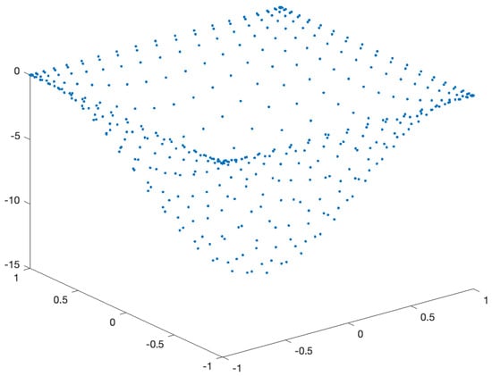
Figure 1. Deformed shape of the $[0°/90°/90°/0°]$ cross−ply laminated plate discretised with $21\times 21$ points, before adimensionalisation, using the RBF-PS method in general grids.

Table 2 and Table 3 present a comparison of the static deflections derived from the current shell model with the outcomes of Reddy’s shell formulation, utilizing both first-order and third-order shear-deformation theories [2], in addition to the LW analytical solution from [24]. We examine nodal grids comprising $11\times 11,13\times 13,17\times 17$, and $21\times 21$ points, alongside different values of $R/a$ and two values of $a/h$ (10 and 100), in addition to stacking sequences of the form $\left[0°/90°/0°\right]$ for Table 2 and $\left[0°/90°/90°/0°\right]$ for Table 3. The findings from our three PS methods show strong concordance across different $a/h$ ratios when compared to Reddy’s higher-order results and the LW analytical solution.

Table 2. Non-dimensional central deflection for a spherical shell ($R_1=R_2$), $\overline{w}=w{\displaystyle \frac{{10}^3{E}_2{h}^3}{P_0{a}^4}}$ variation with various number of grid points $N\times N$, for different $R/a$ ratios, and for a $[0°/90°/0°]$ laminate.

	Method	Grid	$\mathit{R}/\mathit{a}$
$\mathit{a}/\mathit{h}$			5	10	100	${\mathbf{10}}^{\mathbf{9}}$
10	Trefethen’s cheb.m	($13\times 13$)	7.0097	7.2452	7.3265	7.3273
		($17\times 17$)	7.0097	7.2452	7.3265	7.3273
		($21\times 21$)	7.0097	7.2452	7.3265	7.3273
	RBF-tensor-product grids	($13\times 13$)	7.0059	7.2444	7.3266	7.3275
		($17\times 17$)	7.0083	7.2454	7.3272	7.3281
		($21\times 21$)	7.0096	7.2453	7.3266	7.3275
	RBF-PS general grids	($13\times 13$)	7.0088	7.2447	7.3261	7.3268
		($17\times 17$)	7.0094	7.2451	7.3264	7.3272
		($21\times 21$)	7.0095	7.2452	7.3264	7.3273
	HSDT [2]		6.7688	7.0325	7.1240	7.125
	FSDT [2]		6.4253	6.6247	6.6923	6.6939
	LW [24]		7.0834	7.3252	7.4087	7.4095
100	Trefethen’s cheb.m	($13\times 13$)	1.0308	2.3971	4.2610	4.2947
		($17\times 17$)	1.0308	2.3971	4.2610	4.2947
		($21\times 21$)	1.0308	2.3971	4.2610	4.2947
	RBF-tensor-product grids	($13\times 13$)	1.0302	2.3965	4.2616	4.2953
		($17\times 17$)	1.0302	2.3963	4.2605	4.2942
		($21\times 21$)	1.0307	2.3970	4.2609	4.2946
	RBF-PS general grids	($13\times 13$)	1.0298	2.3953	4.2590	4.2928
		($17\times 17$)	1.0304	2.3964	4.2607	4.2944
		($21\times 21$)	1.0305	2.3967	4.2609	4.2946
	HSDT [2]		1.0321	2.4099	4.3074	4.3420
	FSDT [2]		1.0337	2.4109	4.3026	4.3370
	LW [24]		1.0340	2.4120	4.3055	4.3400

Table 3. Non-dimensional central deflection for a spherical shell ($R_1=R_2$), $\overline{w}=w{\displaystyle \frac{{10}^3{E}_2{h}^3}{P_0{a}^4}}$ variation with various number of grid points $N\times N$, for different $R/a$ ratios, and for a $[0°/90°/90°/0°]$ laminate.

	Method	Grid	$\mathit{R}/\mathit{a}$
$\mathit{a}/\mathit{h}$			5	10	100	${\mathbf{10}}^{\mathbf{9}}$
10	Trefethen’s cheb.m	($13\times 13$)	6.9071	7.1383	7.2181	7.2189
		($17\times 17$)	6.9071	7.1383	7.2181	7.2189
		($21\times 21$)	6.9071	7.1383	7.2181	7.2189
	RBF-tensor-product grids	($13\times 13$)	6.9157	7.1404	7.2181	7.2189
		($17\times 17$)	6.9056	7.1382	7.2184	7.2192
		($21\times 21$)	6.9070	7.1384	7.2182	7.2190
	RBF-PS general grids	($13\times 13$)	6.9062	7.1378	7.2177	7.2185
		($17\times 17$)	6.9068	7.1382	7.2180	7.2188
		($21\times 21$)	6.9069	7.1383	7.2180	7.2188
	HSDT [2]		6.7865	7.0536	7.1464	7.1474
	FSDT [2]		6.3623	6.5595	6.6264	6.6280
	LW [24]		6.9953	7.2322	7.3139	7.3148
100	Trefethen’s cheb.m	($13\times 13$)	1.0249	2.3878	4.2554	4.2893
		($17\times 17$)	1.0249	2.3878	4.2554	4.2893
		($21\times 21$)	1.0249	2.3878	4.2554	4.2893
	RBF-tensor-product grids	($13\times 13$)	1.0244	2.3873	4.2559	4.2898
		($17\times 17$)	1.0244	2.3872	4.2551	4.2890
		($21\times 21$)	1.0248	2.3878	4.2553	4.2892
	RBF-PS general grids	($13\times 13$)	1.0240	2.3862	4.2536	4.2874
		($17\times 17$)	1.0245	2.3872	4.2551	4.2890
		($21\times 21$)	1.0246	2.3875	4.2553	4.2892
	HSDT [2]		1.0264	2.4024	4.3082	4.3430
	FSDT [2]		1.0279	2.4030	4.3021	4.3368
	LW [24]		1.0284	2.4048	4.3073	4.3420

5.2. Free Vibration of Spherical and Cylindrical Laminated Shells

This study examines nodal grids consisting of $13\times 13,17\times 17$, and $21\times 21$ points. Table 4 (stacking sequence $\left[0°/90°/90°/0°\right]$) and Table 5 (stacking sequence $\left[0°/90°/0°\right]$) present a comparison of the nondimensionalized natural frequencies derived from the current layerwise theory for various cross-ply spherical shells with the analytical solutions reported by Reddy and Liu [2], who investigated both first-order (FSDT) and third-order (HSDT) theories. The first-order theory often overestimates the fundamental natural frequencies of symmetric thick shells and symmetric shallow thin shells. The current method demonstrates strong concordance with the reference solutions, utilizing our three PS methods.

Table 4. Nondimensionalized fundamental frequencies of cross−ply laminated spherical shells, $\overline{\omega }=\omega {\displaystyle \frac{a^2}{h}}\sqrt{\rho /E_2}$, laminate ($[0°/90°/90°/0°]$).

	Method	Grid	$\mathit{R}/\mathit{a}$
$\mathit{a}/\mathit{h}$			5	10	100	${\mathbf{10}}^{\mathbf{9}}$
10	Trefethen’s cheb.m	($13\times 13$)	11.9532	11.7886	11.7334	11.7328
		($17\times 17$)	11.9532	11.7886	11.7334	11.7328
		($21\times 21$)	11.9532	11.7886	11.7334	11.7328
	RBF-tensor-product grids	($13\times 13$)	11.9453	11.7868	11.7334	11.7328
		($17\times 17$)	11.9545	11.7887	11.7331	11.7325
		($21\times 21$)	11.9533	11.7885	11.7333	11.7328
	RBF-PS general grids	($13\times 13$)	11.9537	11.7889	11.7336	11.7331
		($17\times 17$)	11.9533	11.7886	11.7334	11.7329
		($21\times 21$)	11.9532	11.7886	11.7334	11.7328
	HSDT [2]		12.040	11.840	11.780	11.780
100	Trefethen’s cheb.m	($13\times 13$)	31.1257	20.4451	15.3284	15.2679
		($17\times 17$)	31.1258	20.4451	15.3284	15.2679
		($21\times 21$)	31.1258	20.4451	15.3284	15.2679
	RBF-tensor-product grids	($13\times 13$)	31.1334	20.4474	15.3275	15.2670
		($17\times 17$)	31.1326	20.4480	15.3290	15.2685
		($21\times 21$)	31.1261	20.4453	15.3286	15.2690
	RBF-PS general grids	($13\times 13$)	31.1428	20.4545	15.3326	15.2730
		($17\times 17$)	31.1325	20.4480	15.3290	15.2684
		($21\times 21$)	31.1300	20.4468	15.3286	15.2680
	HSDT [2]		31.100	20.380	15.230	15.170

Table 5. Nondimensionalized fundamental frequencies of cross−ply laminated spherical shells, $\overline{\omega }=\omega {\displaystyle \frac{a^2}{h}}\sqrt{\rho /E_2}$, laminate ($[0°/90°/0°]$).

	Method	Grid	$\mathit{R}/\mathit{a}$
$\mathit{a}/\mathit{h}$			5	10	100	${\mathbf{10}}^{\mathbf{9}}$
10	Trefethen’s cheb.m	($13\times 13$)	11.8715	11.7068	11.6516	11.6510
		($17\times 17$)	11.8715	11.7068	11.6516	11.6510
		($21\times 21$)	11.8715	11.7068	11.6516	11.6510
	RBF-tensor-product grids	($13\times 13$)	11.8748	11.7075	11.6514	11.6509
		($17\times 17$)	11.8727	11.7066	11.6509	11.6504
		($21\times 21$)	11.8716	11.7067	11.6515	11.6509
	RBF-PS general grids	($13\times 13$)	11.8720	11.7071	11.6518	11.6513
		($17\times 17$)	11.8716	11.7069	11.6516	11.6511
		($21\times 21$)	11.8715	11.7068	11.6516	11.6510
	HSDT [2]		12.060	11.860	11.790	11.790
100	Trefethen’s cheb.m	($13\times 13$)	31.0383	20.4060	15.3186	15.2584
		($17\times 17$)	31.0383	20.4060	15.3186	15.2584
		($21\times 21$)	31.0383	20.4060	15.3186	15.2584
	RBF-tensor-product grids	($13\times 13$)	31.0469	20.4086	15.3175	15.2573
		($17\times 17$)	31.0463	20.4096	15.3195	15.2593
		($21\times 21$)	31.0386	20.4063	15.3188	15.2690
	RBF-PS general grids	($13\times 13$)	31.0499	20.4133	15.3237	15.2635
		($17\times 17$)	31.0400	20.4070	15.3191	15.2590
		($21\times 21$)	31.0387	20.4062	15.3187	15.2586
	HSDT [2]		31.0398	20.350	15.240	15.170

Table 6 displays the nondimensionalized natural frequencies derived from the current layerwise theory for cross-ply cylindrical shells featuring lamination schemes $[0/90/0]$ and $[0/90/90/0]$. Our results were compared with the analytical solutions provided by Reddy and Liu Reddy and Liu [2], who employed both FSDT and HSDT theories. The comparison shows strong agreement across all PS methods, even with a limited number of grid points.

Table 6. Nondimensionalized fundamental frequencies of cross−ply cylindrical shells, $\overline{\omega }=\omega {\displaystyle \frac{a^2}{h}}\sqrt{\rho /E_2}$.

		[0/90/0]		[0/90/90/0]
R/a	Method	$\mathit{a}/\mathit{h}=\mathbf{100}$	$\mathit{a}/\mathit{h}=\mathbf{10}$	$\mathit{a}/\mathit{h}=\mathbf{100}$	$\mathit{a}/\mathit{h}=\mathbf{10}$
5	Trefethen’s cheb.m	($13\times 13$)	20.3552	11.6657	20.3988	11.7530
		($17\times 17$)	20.3553	11.6657	20.3989	11.7530
		($21\times 21$)	20.3553	11.6657	20.3989	11.7530
	RBF-tensor-product grids	($13\times 13$)	20.3662	11.6692	20.4046	11.7452
		($17\times 17$)	20.3661	11.6668	20.4050	11.7540
		($21\times 21$)	20.3557	11.6657	20.3992	11.7530
	RBF-PS general grids	($13\times 13$)	20.3689	11.6661	20.4102	11.7534
		($17\times 17$)	20.3572	11.6658	20.4005	11.7530
		($21\times 21$)	20.3557	11.6657	20.3992	11.7530
	FSDT [2]		20.332	12.207	20.361	12.267
	HSDT [2]		20.330	11.850	20.360	11.830
100	Trefethen’s cheb.m	($13\times 13$)	15.2734	11.6511	15.2829	11.7329
		($17\times 17$)	15.2734	11.6511	15.2829	11.7329
		($21\times 21$)	15.2734	11.6511	15.2829	11.7329
	RBF-tensor-product grids	($13\times 13$)	15.2722	11.6509	15.2820	11.7329
		($17\times 17$)	15.2742	11.6504	15.2835	11.7326
		($21\times 21$)	15.2735	11.6509	15.2831	11.7328
	RBF-PS general grids	($13\times 13$)	15.2784	11.6513	15.2881	11.7331
		($17\times 17$)	15.2739	11.6511	15.2835	11.7329
		($21\times 21$)	15.2735	11.6511	15.2830	11.7329
	FSDT [2]		15.198	12.163	15.199	12.227
	HSDT [2]		15.19	11.79	15.19	11.78
Plate	Trefethen’s cheb.m	($13\times 13$)	15.2584	11.6510	15.2674	11.7328
		($17\times 17$)	15.2584	11.6510	15.2674	11.7328
		($21\times 21$)	15.2584	11.6510	15.2674	11.7328
	RBF-tensor-product grids	($13\times 13$)	15.2573	11.6509	15.2670	11.7328
		($17\times 17$)	15.2593	11.6504	15.2685	11.7325
		($21\times 21$)	15.2586	11.6509	15.2680	11.7328
	RBF-PS general grids	($13\times 13$)	15.2635	11.6513	15.2730	11.7331
		($17\times 17$)	15.2590	11.6511	15.2684	11.7329
		($21\times 21$)	15.2586	11.6510	15.2680	11.7328
	FSDT [2]		15.183	12.162	15.184	12.226
	HSDT [2]		15.170	11.790	15.170	11.780

Figure 2 presents the eigenvalues (“eig”) for the initial four vibrational modes of a cross-ply laminated plate, represented by $\overline{\omega }=\omega {\displaystyle \frac{a^2}{h}}\sqrt{\rho /E_2}$, with a laminate configuration of $\left[0°/90°/90°/0°\right]$, utilizing a grid of $21\times 21$ points and a ratio of $a/h=100$.

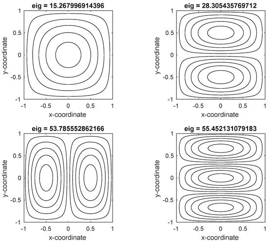
Figure 2. Illustration of the first 4 vibrational modes of cross−ply laminated plate, $\overline{\omega }=\omega {\displaystyle \frac{a^2}{h}}\sqrt{\rho /E_2}$, laminate ($[0°/90°/90°/0°]$) grid $21\times 21$ points, $a/h=100$.

6. Concluding Remarks

This paper presents a novel layerwise shell theory for laminated orthotropic elastic shells. This theory employs collocation with radial basis functions (RBF) in a pseudospectral framework, presented in three formulations, to tackle the equations of motion and boundary conditions. Results for static deformations and natural frequencies are presented and compared with existing sources. Our meshless approaches demonstrate high effectiveness in analyzing static deformations and free vibrations of laminated composite shells. The benefits of pseudospectral interpolation schemes encompass the lack of a mesh, ease of discretizing boundary conditions, and the formulation of equilibrium or motion equations. The results indicate that the static displacements and natural frequencies derived from the three pseudospectral methods align closely with analytical and reference solutions.

References

- Pandya, B.N.; Kant, T. Higher-order shear deformable theories for flexure of sandwich plates-finite element evaluations. Int. J. Solids Struct. 1988, 24, 419–451. [Google Scholar] [CrossRef]
- Reddy, J.N.; Liu, C.F. A higher-order shear deformation theory of laminated elastic shells. Int. J. Eng. Sci. 1985, 23, 319–330. [Google Scholar] [CrossRef]
- Touratier, M. An efficient standard plate theory. Int. J. Eng. Sci. 1991, 29, 901–916. [Google Scholar] [CrossRef]
- Mindlin, R.D. Influence of rotary inertia and shear in flexural motions of isotropic elastic plates. J. Appl. Mech. 1951, 18, 31–38. [Google Scholar] [CrossRef]
- Reddy, J.N. Mechanics of Laminated Composite Plates; CRC Press: New York, NY, USA, 1997. [Google Scholar]
- Carrera, E. Historical review of zig-zag theories for multilayered plates and shells. Appl. Mech. Rev. 2003, 56, 287–308. [Google Scholar] [CrossRef]
- Carrera, E. Developments, ideas, and evaluations based upon Reissner’s Mixed variational Theorem in the modelling of multilayered plates and shells. Appl. Mech. Rev. 2001, 54, 301–329. [Google Scholar] [CrossRef]
- Carrera, E. C0 Reissner-Mindlin multilayered plate elements including zig-zag and interlaminar stress continuity. Int. J. Numer. Methods Eng. 1996, 39, 1797–1820. [Google Scholar] [CrossRef]
- Kansa, E.J. Multiquadrics- A scattered data approximation scheme with applications to computational fluid dynamics. I: Surface approximations and partial derivative estimates. Comput. Math. Appl. 1990, 19, 127–145. [Google Scholar] [CrossRef]
- Ferreira, A.J.M. A formulation of the multiquadric radial basis function method for the analysis of laminated composite plates. Compos. Struct. 2003, 59, 385–392. [Google Scholar] [CrossRef]
- Ferreira, A.J.M.; Roque, C.M.C.; Martins, P.A.L.S. Analysis of composite plates using higher-order shear deformation theory and a finite point formulation based on the multiquadric radial basis function method. Compos. Part 2003, 34, 627–636. [Google Scholar] [CrossRef]
- Hardy, R.L. Multiquadric equations of topography and other irregular surfaces. Geophys. Res. 1971, 176, 1905–1915. [Google Scholar] [CrossRef]
- Hardy, R.L. Theory and applications of the multiquadric-biharmonic method: 20 years of discovery. Comput. Math. Applic. 1990, 19, 163–208. [Google Scholar] [CrossRef]
- Kansa, E.J. Multiquadrics- A scattered data approximation scheme with applications to computational fluid dynamics. II: Solutions to parabolic, hyperbolic and elliptic partial differential equations. Comput. Math. Appl. 1990, 19, 147–161. [Google Scholar] [CrossRef]
- Ferreira, A.J.M. Analysis of composite plates using a layerwise deformation theory and multiquadrics discretization. Mech. Adv. Mater. Struct. 2005, 12, 99–112. [Google Scholar] [CrossRef]
- Ferreira, A.J.M. Polyharmonic (thin-plate) splines in the aalysis of composite plates. Int. J. Mech. Sci. 2004, 46, 1549–1569. [Google Scholar] [CrossRef]
- Fantuzzi, N.; Tornabene, F.; Bacciocchi, M.; Ferreira, A.J.M. On the Convergence of Laminated Composite Plates of Arbitrary Shape through Finite Element Models. J. Compos. Sci. 2018, 2, 16. [Google Scholar] [CrossRef]
- Moreira, J.A.; Moleiro, F.; Araújo, A.L.; Pagani, A. Active aeroelastic flutter control of supersonic smart variable stiffness composite panels using layerwise models. Compos. Struct. 2024, 343, 118287. [Google Scholar] [CrossRef]
- Gao, Y.S.; Cai, C.S.; Huang, C.Y.; Zhu, Q.H.; Schmidt, R.; Zhang, S.Q. A compressible layerwise third-order shear deformation theory with transverse shear stress continuity for laminated sandwich plates. Compos. Struct. 2024, 338, 118108. [Google Scholar] [CrossRef]
- Fornberg, B. A Practical Guide to Pseudospectral Methods; Cambridge Monographs on Applied and Computational Mathematics; Cambridge University Press: Cambridge, UK, 1996. [Google Scholar]
- Trefethen, L.N. Spectral Methods in MatLab; Society for Industrial and Applied Mathematics: Philadelphia, PA, USA, 2000. [Google Scholar]
- Rippa, S. An algorithm for selecting a good value for the parameter c in radial basis function interpolation. Adv. Comput. Math. 1999, 11, 193–210. [Google Scholar] [CrossRef]
- Ferreira, A.J.M.; Fasshauer, G.E. Computation of natural frequencies of shear deformable beams and plates by a RBF-Pseudospectral method. Comput. Methods Appl. Mech. Eng. 2006, 196, 134–146. [Google Scholar] [CrossRef]
- Carrera, E. Multilayered Shell Theories Accounting for Layerwise Mixed Description, Part 2: Numerical Evaluations. Aiaa J. 1999, 37, 1117–1124. [Google Scholar] [CrossRef]
- Cinefra, M.; Kumar, S.K.; Carrera, E. MITC9 Shell elements based on RMVT and CUF for the analysis of laminated composite plates and shells. Compos. Struct. 2019, 209, 383–390. [Google Scholar] [CrossRef]
Disclaimer/Publisher’s Note: The statements, opinions and data contained in all publications are solely those of the individual author(s) and contributor(s) and not of MDPI and/or the editor(s). MDPI and/or the editor(s) disclaim responsibility for any injury to people or property resulting from any ideas, methods, instructions or products referred to in the content. |
© 2024 by the authors. Licensee MDPI, Basel, Switzerland. This article is an open access article distributed under the terms and conditions of the Creative Commons Attribution (CC BY) license (https://creativecommons.org/licenses/by/4.0/).