Assessing Failure in Steel Cable-Reinforced Rubber Belts Using Multi-Scale FEM Modelling

Abstract

This work introduces a finite element model of a steel cable-reinforced conveyor belt to accurately compute stresses in the splice. In the modelled test rig, the belt runs on two drums and is loaded with a cyclic longitudinal force. An explicit solver is used to efficiently handle the high number of elements and contact conditions. This, however, introduces some issues of dynamics in the model, which are subsequently solved: (a) the longitudinal load is applied with a smooth curve and damping is introduced in the beginning of the simulation, (b) residual stresses are applied in regions of the belt that are initially bent around the drums, and (c) supporting drums are introduced at the start of the simulation to hinder oscillations of the belt at low applied forces. To accurately capture the tensile and bending stiffness of the cables, they are modelled by a combination of solid and beam elements. The results show that numerical artefacts can be reduced to an acceptable extent. In the region of highest stresses, the displacements are additionally mapped onto a submodel with a smaller mesh size. The results show that, for the investigated belt, the local maximum principal stresses significantly increase when this region of highest stresses comes into contact with, and is bent by, the drum. Therefore, it is essential to also consider the belt’s bending to predict failure in such applications.

1. Introduction

Conveyor belts are used in a wide range of applications such as supermarkets, logistic centres, and mining. The conveyor belts in mining are reinforced with steel cables to reach the high strengths required. Such conveyor belts can have lengths of several kilometres. They consist of belt segments that are connected on site. In this connection, which is called splice, the steel cables are arranged in a specific laying scheme. The strength of this splice limits the belt’s strength in cyclic loading and is thus of great interest to engineers. The splice strength is experimentally determined in a test rig where a conveyor belt with one splice runs on two drums and is cyclically loaded [1], see Figure 1. The failure of the belt can be caused by cable–rubber debonding, tearing of the rubber, and the rupture of cables.

To certify a belt for a tensile force, a certain number of cycles must be reached in the test rig without failure. To better understand the failure mechanisms, some effort has been put into monitoring the evolution of damage during the test [2,3]. This could be an initial debonding of cables from the rubber, which, at higher cycle numbers, leads to the rupture of individual cables, which ultimately leads to failure of the belt. The large variety of belt damage mechanisms has been illustrated in a study of damage due to objects such as rocks falling on a conveyor belt [4]. This complex damage behaviour indicates that it is not trivial to predict this failure which depends on the cable and rubber properties, the splice geometry, and the debonding strength of the cable–rubber interface [5]. For conveyor belts of lower strength classes, which are reinforced with textiles, Finite Element Method (FEM) models that compute the stress-distribution in belts that are loaded in tension exist [6,7]. The steel cables, on the other hand, pose a challenge in such models due to their complex stiffness: steel cables have high tensile stiffness but very low bending stiffness, and can feature tension/torsion coupling [8]. This can play a role in the failure of splices.

Various research groups have developed numerical models to predict the strength of a splice, putting the emphasis on different aspects of the complex conveyor belt system. Nordell et al. [9,10] presented a very detailed FEM model of a splice, which even accounts for the tension/torsion coupling of cables. Similar to Keller [11], they argued that simpler specimens can be designed to show damage behaviour similar to that observed in the belt splice, which can then be used to study the damage behaviour in detail, where the influence of belt-drum contact and bending was also discussed. Another research group introduced similar FEM models to study a range of rubber materials and introduce an automated tool for investigating splice schemes [12,13]. In more recent work, other groups such as Li et al. [14] and Wheatley and Keipour [15] presented similar models, focusing on simplified specimens loaded in tension. None of those models account for bending of the belt on the drums in the test rig. Usually, the splice optimisation is carried out according to evaluated stresses in the FEM models. The bending of the belt, however, can affect the local stress fields in the splice in a nonlinear way. This can shift the damage mechanisms compared to a belt loaded purely in tension.

This work introduces a conveyor belt test rig model that fully accounts for contact and bending of the belt on the two drums. The computed stress fields can be used as an indicator of the belt’s strength (Li et al. [16] use a stress-based criterion for damage initiation that agrees well with experimental results of failure). It can, thus, predict the influence of bending on the tested strength of a belt. Note that this work computes static stresses and could be extended towards fatigue models that are based on those stresses, as described by Carraro et al. [17] and Ferdous et al. [18]. Since all steel cables of a belt need to be modelled to capture the stress variations in the splice, a full 3-d model including drums contact is very challenging in terms of computational time. For this reason, a two-scale approach using an explicit full-scale test rig model and a finer-meshed implicit submodel of the region of highest stresses is taken. The models are used to assess whether the bending of the belt at the drums introduces additional stresses in the splice. This work, which is the first full 3-d splice model with bending, can thus answer the question of whether the bending loads are relevant for the mechanical design of conveyor belts. Challenges such as obtaining an initial state of movement and stresses in the belt and coping with initial dynamic artefacts are solved in the explicit model.

2. Methods

In this section, the modelling of the conveyor belt setup and the splice scheme used are explained. Additionally, the setup of the global test rig model and the submodel is presented. The belt is stress-free and flat after production. In the global test rig model, the initially-bent regions are applied with residual stresses. Furthermore, specific techniques are described to avoid unwanted dynamic effects in the explicit global test rig model.

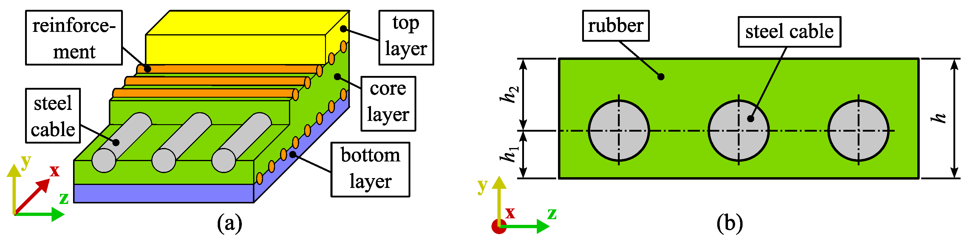
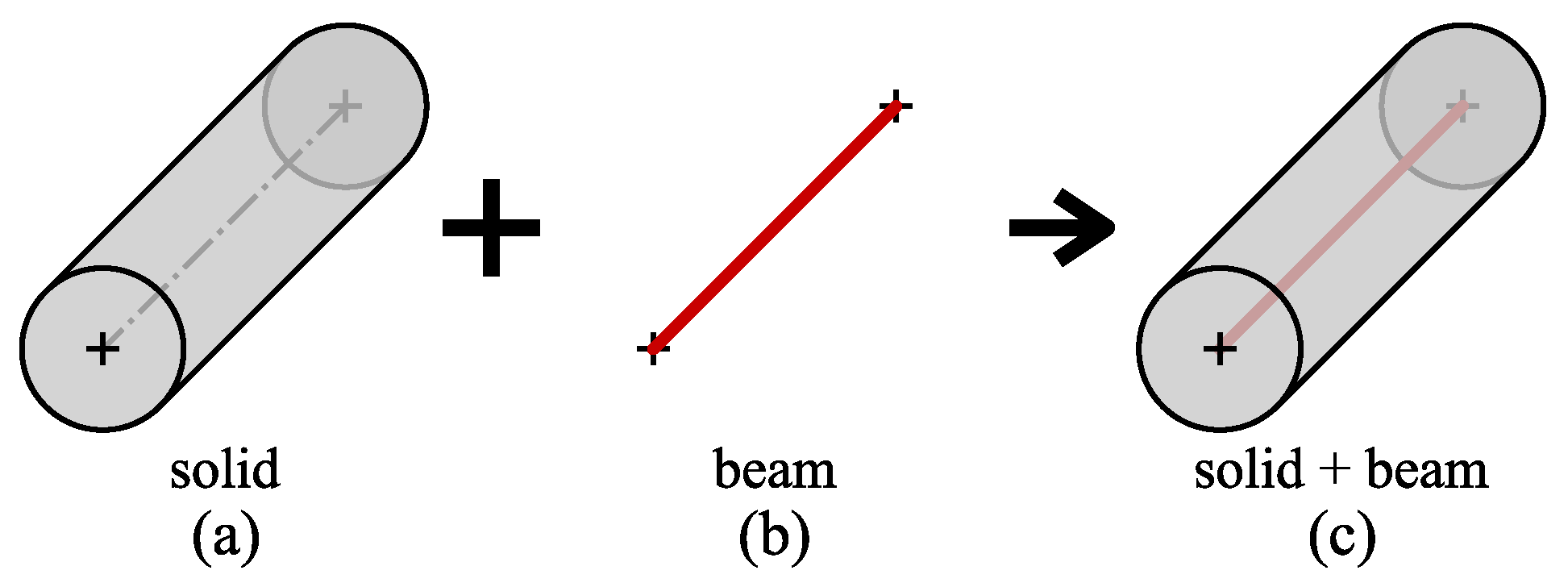
2.1. Material Models and Splice Geometry

This work uses a simple conveyor belt with nine cables and only one rubber material. This belt, which can be simulated much faster, can be assumed to feature similar effects of the bending to realistic belts. The setup of a conveyor belt is shown in Figure 2a with the longitudinal direction, the out-of plane direction, and the lateral direction, defined as x, y, and z-directions, respectively. Such a steel cable-reinforced conveyor belt can consist of several reinforced and non-reinforced rubber layers. The belt considered in this work is made up of only one rubber material reinforced by parallel steel cables and no additional transverse reinforcement, see Figure 2b. The belt has a total thickness of $h=42.5$ mm with $h_1=16.75$ mm and $h_2=25.75$ mm. The rubber is modelled as a hyper-elastic material using the Mooney-Rivlin formulation. The strain energy function is given by

$$U=C_{10}\left(I_1-3\right)+C_{01}\left(I_2-3\right)+\frac{1}{D}{\left(J-1\right)}^2,$$

(1)

where $C_{10}$, $C_{01}$, and D are material parameters, and $I_1$ and $I_2$ are the first and second invariant of the left Cauchy—-Green deformation tensor, respectively. J is the determinant of the deformation gradient. The material parameters are listed in

Table 1. Material parameters.

${\mathit{C}}_{10}$ [MPa]	${\mathit{C}}_{01}$ [MPa]	D [1/MPa]
0.7083	0.1417	0.03565

. The parameters $C_{10}$ and $C_{01}$ are taken from Froböse et al. [12] for a rubber material with a shear modulus of $G=1.7$ MPa. The rubber density is not given and is assumed as ${\rho }_{\mathrm{rubber}}=1000$ kg/m³. To use a typical Poisson’s ratio for rubber of $\nu$ very close to 0.5 would introduce high-frequency noise in the explicit simulation, as described in [19], suggesting an upper limit of $\nu =0.495$. Therefore, the parameter D is set to reach a Poisson’s ratio of $\nu =0.485$.

Due to their inherent structure, the steel cables cannot be modelled accurately by a simple solid material model. Steel cables feature high tensile stiffness and low bending stiffness compared to a solid material of the same diameter. Also, they can feature a tension/torsion coupling, which requires special modelling in FEM. In this work, the steel cables are modelled so that they reach accurate tensile and bending stiffness. To this end, the volume of the cylindrical steel cables is meshed with solid elements and, in the cable’s axis, additional beam elements are introduced. This setup is illustrated in Figure 3. The mechanical response is assumed to be linear elastic. The beam elements share nodes with the solid elements. It should be mentioned that the volume elements are not affected by the rotations of their connected nodes. The steel cables in this work have a radius of $r_{\mathrm{cable}}=6.75$ mm.

A very small radius of the beam is chosen so that the solid elements account for the whole bending stiffness of the cable. To determine the Young’s modulus for the solid elements $E_{\mathrm{solid}}$, a three-point-bending test of a rubberised steel cable with a bending length $l_{\mathrm{bend}}=110$ mm has been performed. From the linear region at the beginning of the force-displacement curve, a bending stiffness $S_{\mathrm{bend}}=95 \frac{\mathrm{N}}{\mathrm{mm}}$ is obtained and yields a Young’s modulus for the solid elements as

$$E_{\mathrm{solid}}=\frac{S_{\mathrm{bend}}{l}_{\mathrm{bend}}^3}{12r_{\mathrm{cable}}^4\pi }=1615.68 \mathrm{MPa}.$$

(2)

To determine the average Young’s modulus of the cable, a tensile test of a single cable with a test length of $l_{\mathrm{tensile}}=200$ mm has been performed. A tensile stiffness $s_{\mathrm{tensile}}=25$ kN/mm is obtained from the linear region at the beginning of the force-displacement curve and yields a Young’s modulus for the cable:

$$E_{\mathrm{cable}}=\frac{s_{\mathrm{tensile}}{l}_{\mathrm{tensile}}}{r_{\mathrm{vol}}^2\pi }=\mathrm{34,931.13} \mathrm{MPa}.$$

(3)

In order to not induce any additional bending stiffness by the beam, the area ratio of the solid and the beam cross-sections is set to ${\xi }_{\mathrm{volbeam}}=1000$. This results in a beam radius of $r_{\mathrm{beam}}=0.214$ mm. The Young’s modulus of the beam $E_{\mathrm{beam}}$ needs to be adjusted to reach the total cable stiffness by the combination of the beam and solid elements. Therefore, $E_{\mathrm{beam}}$ has to account for the tensile stiffness that has not been accounted for by the solid elements as

$$E_{\mathrm{beam}}={\xi }_{\mathrm{volbeam}}\left(E_{\mathrm{cable}}-E_{\mathrm{solid}}\right)=\mathrm{33,300} \mathrm{GPa}.$$

(4)

The density of the steel cable ${\rho }_{\mathrm{cable}}$ is computed from the density of the rubber ${\rho }_{\mathrm{rubber}}$, the density of steel ${\rho }_{\mathrm{steel}}=7850$ kg/m³, and an assumed volume ratio of steel in the rubberised cables ${\xi }_{\mathrm{st}}=0.6$. Therefore, the density of the steel cable is given by

$${\rho }_{\mathrm{cable}}={\xi }_{\mathrm{st}}{\rho }_{\mathrm{steel}}+\left(1-{\xi }_{\mathrm{st}}\right){\rho }_{\mathrm{rubber}}=5110 \frac{\mathrm{kg}}{{\mathrm{m}}^3}.$$

(5)

The Poisson’s ratio of the solid and the beam elements is assumed to be 0.3.

The splice scheme used for the splice is shown in Figure 4 and the corresponding parameters of the splice are listed in

Table 2. Parameters of the splice.

Parameter Name	Symbol	Value	Unit
belt width	$w_{\mathrm{belt}}$	190	mm
splice length	$l_{\mathrm{splice}}$	4.7	m
cable positions	$x_i$	0.2, 0.7, 2, 3, 4, 4.5	m
outer steel cable spacing	$s_{\mathrm{belt}}$	20	mm
inner steel cable spacing	$s_{\mathrm{splice}}$	17	mm
gap between cable ends	$l_{\mathrm{gap}}$	70	mm

. Outside the splice, the steel cables are arranged in parallel with an equal distance between the cable axes of $s_{\mathrm{belt}}$. Within the splice, the steel cables are rearranged to a lateral distance between the cables of $s_{\mathrm{splice}}$. Cubic splines are used to describe the lateral change in the steel cable axes between outer regions and the splice.

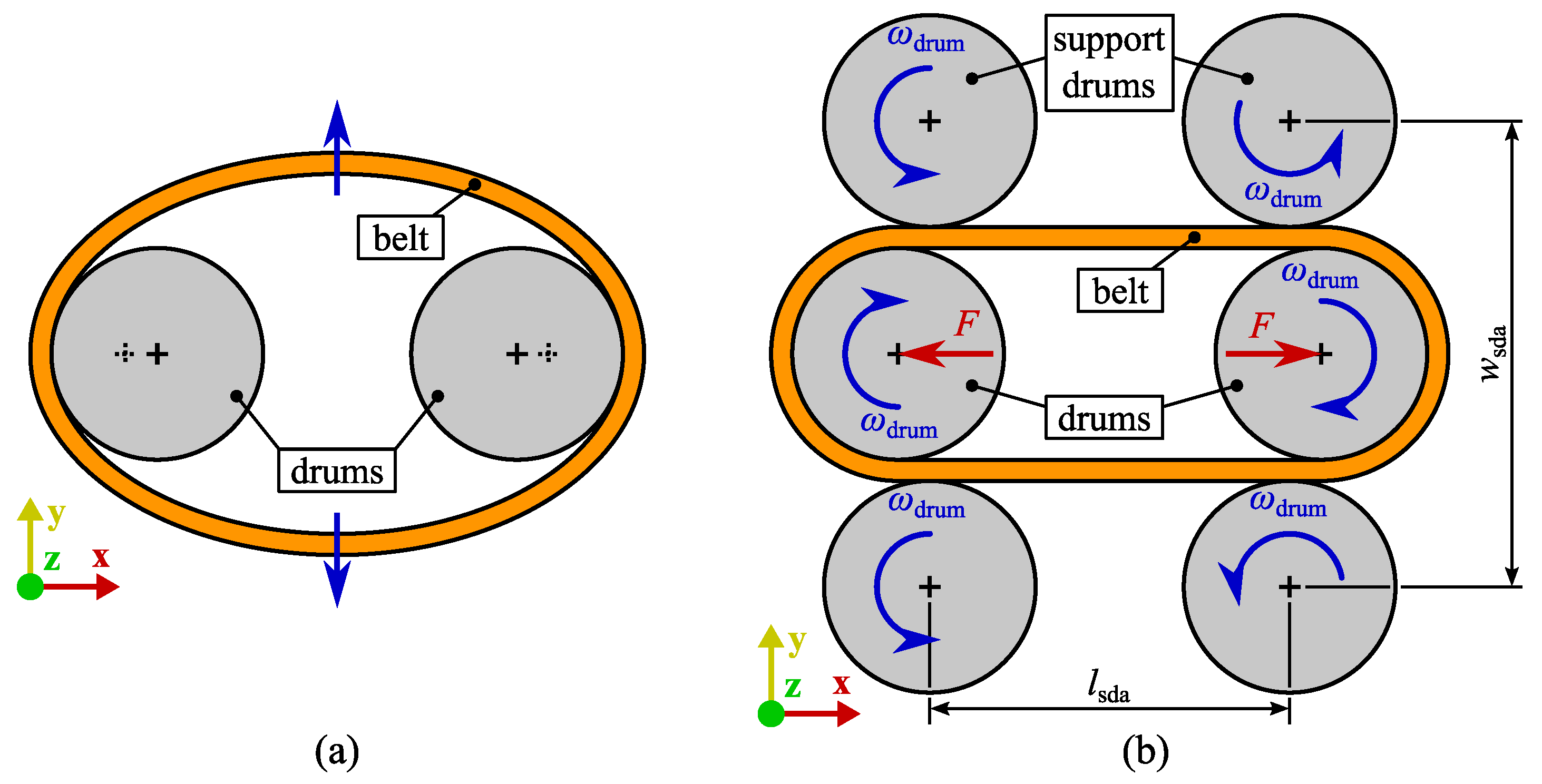
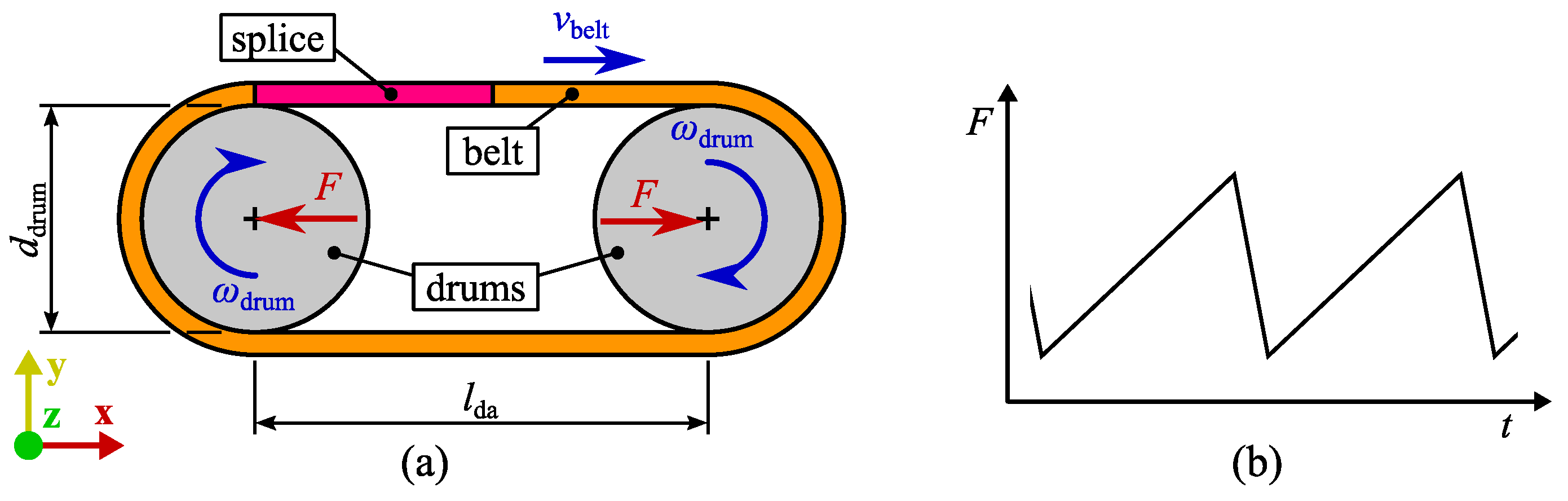
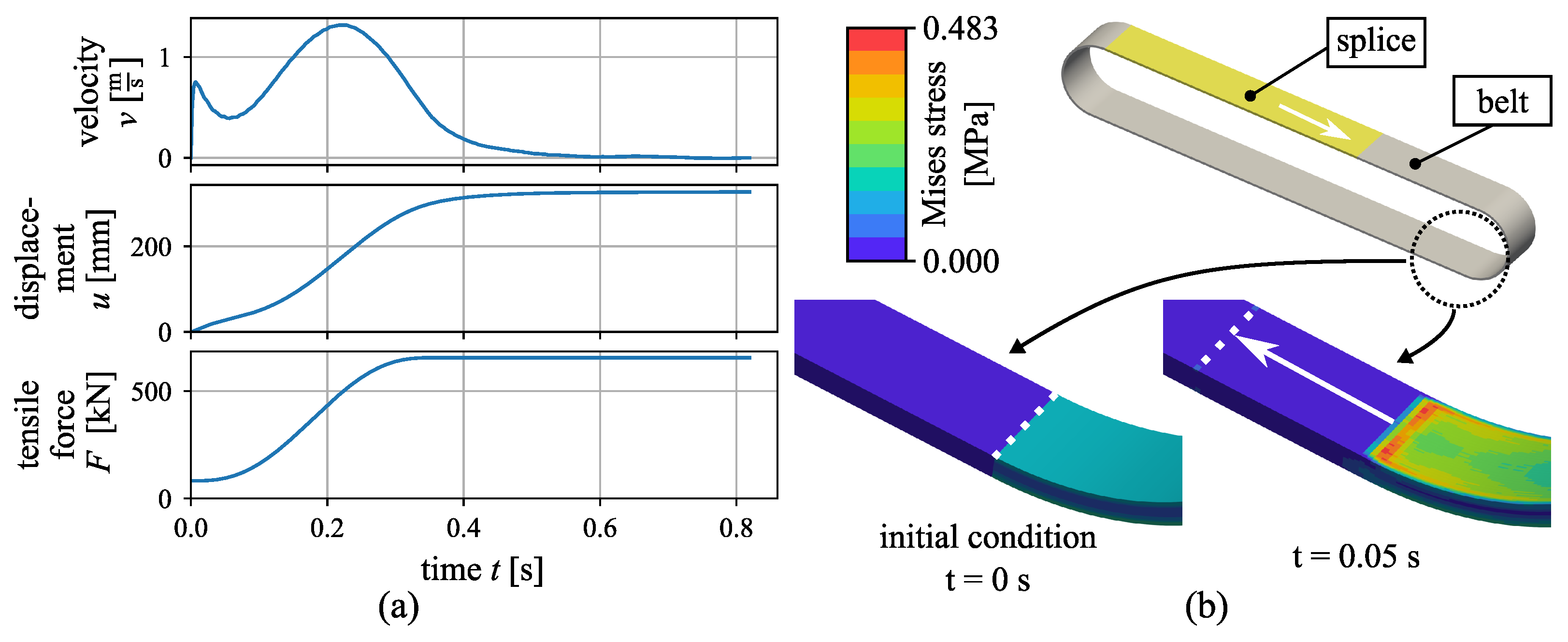
2.2. Test Rig Model

In this section, the global FEM model of the conveyor belt test rig is described. In the test rig [1], the belt is cyclically loaded in tension as it is running on the drums. This work considers the quasi-static case of the conveyor belt running around the drums with a constant applied load F. For reasons of efficiency, an explicit solver is used. This means that dynamic effects in the model are considered as artefacts and have to be reduced to a small extent. To be able to start the simulation with a belt running on the two drums, the bending stresses of the belt on the drums have to be considered. This is reached by the application of residual stresses. Additionally, the application of the load is optimised and additional drums are introduced that avoid belt oscillations in the beginning of the simulation. The model is used to determine stress and strain fields for the conveyor belt running in the test rig. The validity for the quasi-static case is examined. The region of highest stresses in the belt running around the drum is determined and investigated further in a submodel.

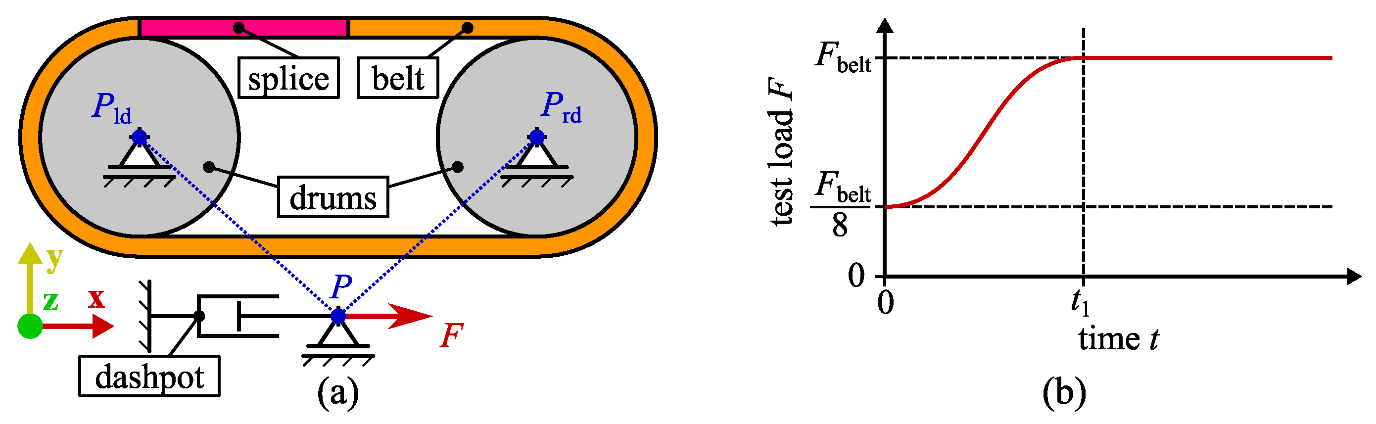
2.2.1. Model Setup

The conveyor belt test rig shown in Figure 1 is represented as a quasi-static FEM model. The belt geometry, splice scheme, and materials of the model are taken from above. The left end of the splice is initially positioned right above the centre of the left drum. All model parameters are listed in

Table 3. Parameters of the test rig.

Parameter Name	Symbol	Value	Unit
distance of the drum axes	$l_{\mathrm{da}}$	7	m
diameter of the drums	$d_{\mathrm{drum}}$	1.25	m
velocity of the belt Equation (7)	$v_{\mathrm{belt}}$	6.454	m/s
number of circulations per load cycle [1]	$n_{\mathrm{cplc}}$	18	1
time period of one load cycle [1]	$t_{\mathrm{lc}}$	50	s
angular velocity of the drums Equation (8)	${\omega }_{\mathrm{drum}}$	9.987	rad/s
point mass of the drum Equation (9)	$m_{\mathrm{drum}}$	1502	kg
moment of inertia of the drums Equation (10)	$I_{\mathrm{z}\mathrm{drum}}$	429	$\mathrm{kg}{\mathrm{m}}^2$
tensile load in the belt Equation (12)	$F_{\mathrm{belt}}$	655.2	kN

. To handle the non-linearities in the material, the contact between the belt and drums and a high number of elements, an explicit solver is used, which is much more efficient for such models. Velocities in the model, thus, have no physical meaning and dynamic effects are considered as artefacts.

The drums are modelled as rigid discrete surfaces with reference points in each of their axes. In the x- and y-axes, the drum’s rotation is fixed. The displacement of the drum’s reference points is also constrained in y- and in the z-direction. An additional reference point P for applying the tensile load of the belt F is introduced, see Figure 5a. The reference point P is coupled to the reference points of the left drums $P_{\mathrm{ld}}$ and right drum $P_{\mathrm{rd}}$ in the x-direction:

$$\begin{array}{cc}\hfill u_{\mathrm{x}}+{\eta }_{\mathrm{c}}{u}_{\mathrm{ldx}}& =0\mathrm{and}\hfill \\ \hfill u_{\mathrm{x}}-{\eta }_{\mathrm{c}}{u}_{\mathrm{rdx}}& =0,\hfill \end{array}$$

(6)

with $u_{\mathrm{x}}$ as the displacement of P, $u_{\mathrm{ldx}}$ as the displacement of $P_{\mathrm{ld}}$, $u_{\mathrm{rdx}}$ as the displacement of $P_{\mathrm{rd}}$, and ${\eta }_{\mathrm{c}}$ as the weight factor for the coupling. Since F should be applied in the belt, the weight factor for the coupling is set to ${\eta }_{\mathrm{c}}=4$. The contact between the drums and the belt is modelled with penalty contact. The friction coefficient between rubber and steel ${\mu }_{\mathrm{rs}}$ for the dry condition is between 0.6 to 1.1 according to Cruz Gómez et al. [20]. Therefore, ${\mu }_{\mathrm{rs}}=0.8$ is assumed.

The explicit simulation starts with a running belt with the initial velocity of the belt $v_{\mathrm{belt}}$, which can be calculated from the number of circulations per tensile load cycle $n_{\mathrm{cplc}}$ and the time period of one load cycle $t_{\mathrm{lc}}$, as defined in [1]:

$$v_{\mathrm{belt}}=\frac{n_{\mathrm{cplc}}\left(d_{\mathrm{d}}\pi +2l_{\mathrm{da}}\right)}{t_{\mathrm{lc}}}.$$

(7)

Note that this means that the belt is running with the actual speed stated in Table 3, even though the model is developed for a quasi-static analysis. The angular velocity of the drums ${\omega }_{\mathrm{drum}}$ that corresponds to the belt speed calculates as

$${\omega }_{\mathrm{drum}}=\frac{2v_{\mathrm{belt}}}{d_{\mathrm{drum}}+h},$$

(8)

where the neutral axis is assumed to be in the middle of the belt thickness. Since the right drum is the driving drum, this angular velocity is applied to the right drum continuously throughout the simulation and to the left drum as an initial condition only.

A point mass $m_{\mathrm{drum}}$ is applied at the reference points of the drums. For the mass, a hollow cylinder of steel with an external diameter of $d_{\mathrm{outer}}=d_{\mathrm{drum}}$, an internal diameter $d_{\mathrm{inner}}=d_{\mathrm{drum}}-2·200$ mm, and a height of $h_{\mathrm{drum}}=w_{\mathrm{belt}}+2·50$ mm is assumed. The point mass $m_{\mathrm{drum}}$ is then given by

$$\begin{array}{cc}\hfill & m_{\mathrm{drum}}={\rho }_{\mathrm{steel}}\pi h_{\mathrm{drum}}\frac{d_{\mathrm{outer}}^2-d_{\mathrm{inner}}^2}{4}.\hfill \end{array}$$

(9)

A moment of inertia $I_{\mathrm{z}\mathrm{drum}}$ for rotation in the drum axis is specified for the left drum, which is given for a hollow cylinder by

$$I_{\mathrm{z}\mathrm{drum}}=\frac{1}{2}{m}_{\mathrm{drum}}\left(\frac{d_{\mathrm{outer}}^2+d_{\mathrm{inner}}^2}{4}\right).$$

(10)

The tensile load F is applied smoothly enough and slowly enough so that dynamic effects do not alter the results and, therefore, the displacement caused by the load application increases smoothly. The tensile force on the belt is applied to point P in a way so that oscillations in the belt are minimised: it was discovered that starting with a force $F=F_{\mathrm{belt}}/8$ at $t=0$ and then using a polynomial with the smooth-step option of Abaqus to increase it to $F_{\mathrm{belt}}$ at $t=t_1$ works well, see Figure 5b. Additionally, the reference point P is connected to a damper in the x-direction, which has a damping coefficient d of $100$ Ns/mm. The time $t_1$ is chosen such that the constant applied force is reached before the splice runs into the bent region on the drum:

$$t_1=\frac{l_{\mathrm{da}}-l_{\mathrm{splice}}}{v_{\mathrm{belt}}}=0.3564 \mathrm{s}.$$

(11)

The applied load is selected to be 60% of the nominal strength per width $k_{\mathrm{N}}$ of 7.8 $\frac{\mathrm{kN}}{\mathrm{mm}}$ of such a steel cable-reinforced belt. The width in the nominal strength is taken as the number of cables in the splice $n_{\mathrm{sc}}$ (here $n_{\mathrm{sc}}=7$) times their distance $s_{\mathrm{belt}}$. The force $F_{\mathrm{belt}}$ thus calculates as

$$F_{\mathrm{belt}}=0.6n_{\mathrm{sc}}{s}_{\mathrm{belt}}{k}_{\mathrm{N}}.$$

(12)

The belt is meshed with a global mesh size of 3 mm. Four elements are used over the gap length of the rubber gaps between cables. Outside the splice region, a mesh size of 10 mm is used along the running direction of the belt. To avoid hour glassing, eight-noded fully-integrated hexahedral elements are used for the volume except for the regions near the steel cable ends, where it is not possible to mesh this geometry change using purely hexahedral elements. Thus, those regions are meshed using six-noded wedge elements with reduced integration and four-noded tetrahedral elements. The beams of the steel cables are modelled using two-noded Thimoshenko beam elements. The cables and the rubber are perfectly connected (shared nodes), except for the end faces of the cables, where an initial debonding is assumed. This is because the necessary surface modification of the steel cables to increase the adhesion to the rubber is not present at the ends that have been cut. The drums are meshed with a global mesh size of 10 mm and four-noded rigid quad elements.

To solve the model, the nonlinear explicit solver of the commercial FEM code Abaqus [19] is used where large deformations are considered. A simulation time of 0.80638 s is sufficient for about 60% of the splice running into the bent region of the drum, and the region of highest stresses is located in the middle of the bent region. Mass scaling is used to achieve a stable time increment of $\mathsf{\Delta }t=1.75·{10}^{-6}$ s with a total change in the model’s mass of 4.46%. The test rig model has a total of about 3,250,000 elements and takes 92 h to run on 72 cores.

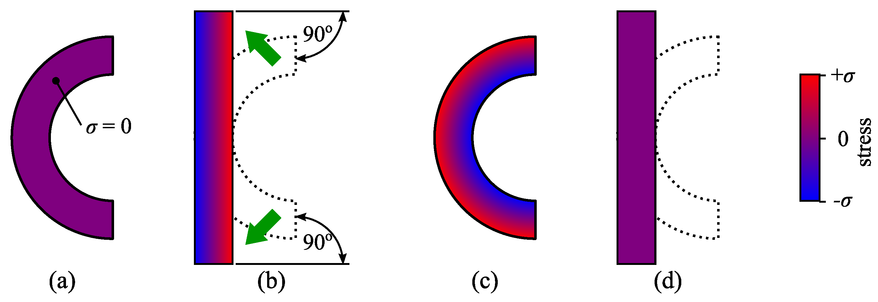
2.2.2. Applying Initial Stresses in Bent Belt Regions

Whenever the conveyor belt is bent, it contains some bending stresses in the cables and the rubber regions. In FEM models, the geometry is usually considered stress-free at the start of the computation. For the regions of the belt that are initially not straight but are bent around the drums, the stresses that correspond to bending with a curvature of 2/d_drum need to be applied as initial stresses. Since the bending stress in a cable-reinforced rubber belt is not trivial, a small implicit simulation is carried out to obtain those stresses. This model contains the belt in its bent shape and straightens it, where the bent shape corresponds to the shape it will initially have in the test rig model (see Figure 6a,b). The stresses in the cable direction are evaluated and their inverse values are applied element-wise in the initial step of the test rig model. It has been verified that this procedure yields an approximately stress-free state in the segment, see Figure 6c,d.

2.2.3. Avoiding Belt Oscillations Using Support Drums

Due to the internal stresses in the initially bent regions, the belt tends to deform as shown in Figure 7a, particularly if only low tensile forces are applied to the drums. In a dynamic model, this induces initial oscillations. To avoid such oscillations, additional support drums are used, but only during the first phase until the final loading state is reached, see Figure 7b. Note that these drums are only introduced to avoid numerical artefacts and are not part of the test rig. The horizontal distance of the support drum axes $l_{\mathrm{sda}}$ is set to 6.8 m, therefore they lie 100 mm closer together than the test rig drums. The diameter of the support drums is the same as the test rig drums, and the vertical distance of the support drum axes $w_{\mathrm{sda}}$ is set to 2.585 m. The support drums initially have the same angular velocity ${\omega }_{\mathrm{drum}}$ as the test rig drums; however, their rotational velocity is free to change during the simulation. Apart from rotation around the z-axis, where an inertia of $I_{\mathrm{z}}\mathrm{drum}$ is applied as in the left drum of the test rig, all translations and rotations of the drums are constrained. The support drums use the same mesh and contact conditions to the belt as the test rig drums. Once the maximum applied load is reached at $t_1$, their contact condition between the support drums and belt is switched off in order to effectively remove them from the simulation.

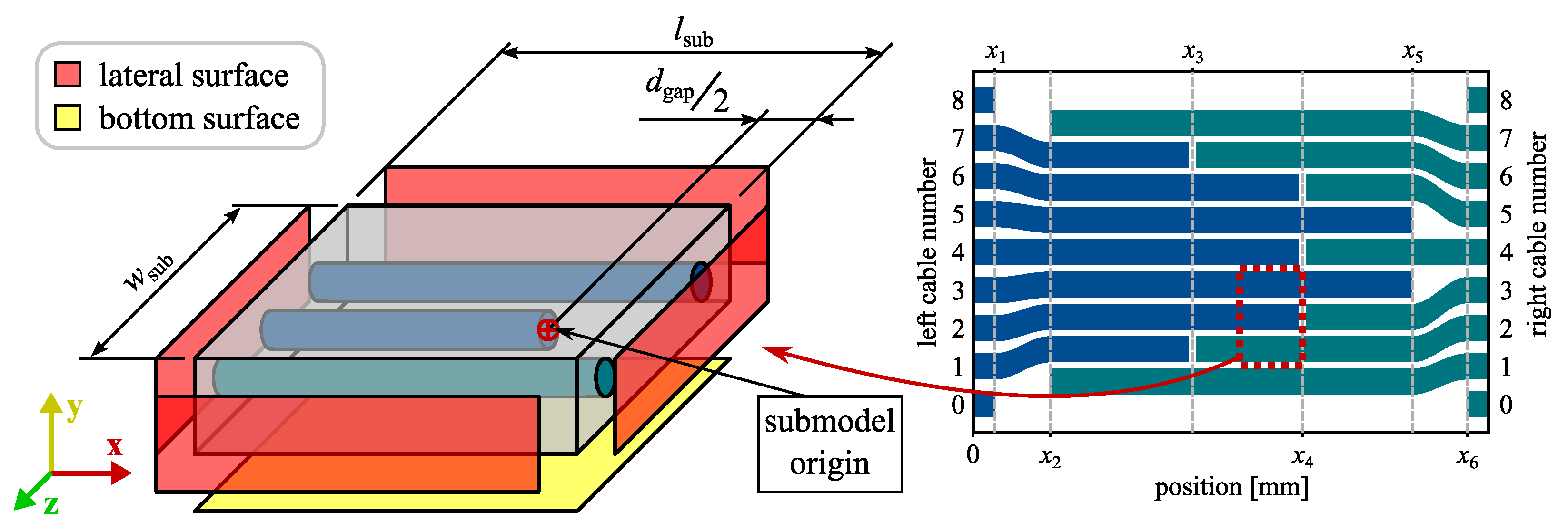
2.3. Submodel

In this work, the region with the highest stresses in the rubber is modelled in the submodel with a finer mesh to investigate this region in more detail. This region is defined in Figure 8, where the same belt geometry and the same material models as the test rig model are used. The submodel length $l_{\mathrm{sub}}$ and the submodel width $w_{\mathrm{sub}}$ are set to 135 mm and 51.5 mm, respectively. The displacements of the test rig model are mapped to the lateral surfaces and the bottom surface of the submodel, see Figure 8. The displacements are mapped separately for the steel cable and the rubber nodes. The nodes at the steel cable/rubber interface use the displacement field of the cable elements in the global model. To avoid convergence issues, the rotational degree of freedom around the beam axes of the beam nodes belonging to the left lateral surface is fixed.

The submodel uses eight-noded fully-integrated hybrid hexahedral elements and is meshed with a global mesh size of 1.5 mm. Eight elements are used in the rubber gap between the steel cables. The beams of the steel cables are modelled using two-noded Thimoshenko beam elements, as in the global model. For computation, the nonlinear implicit solver of the commercial FEM code Abaqus [19] is used, considering large deformations. For verification of the submodelling approach, the stresses of the global model and the submodel are compared to see if the submodelling approach is valid for that case.

3. Results and Discussion

Before showing the results of the test rig model and the submodel, this section starts with an evaluation of the test rig model. It is discussed whether the strategies for avoiding dynamic artefacts have been successful in reaching a quasi-static loading in the model. Figure 9a shows the force applied to point P in the x-direction as well as the computed velocity and displacement at this point as a function of simulation time. After reaching a constant force ($t>0.3564$ s), a small delay occurs before reaching a displacement plateau. Therefore, the used values for damping and applying the initial tensile force, as well as the used support drums, yield accurate steady-state stress fields for $t>0.48$ s, where the deviation from the maximum value $u_{\max }=327.5$ mm is less than 1.5%. The residual stresses remaining after straightening the initially bent belt are shown in Figure 9b. Only slight artefacts are visible in the stresses, which confirms that the residual stresses have been applied in a valid manner. The increased stresses in the bent region for $t=0.05$ s compared to $t=0$ s occur due to the applied loading at this time in the simulation.

The results of the global model for $t=0.806$ s are shown in Figure 10. The maximum principal stress ${\sigma }_{\mathrm{I}}$ is plotted for the plane of the steel cable centre axes in Figure 10a, where ${\sigma }_{\mathrm{I}}$ is computed at the element centre. A small schema shows the position of the splice at the time of the stress evaluation. The highest maximum principal stress ${\sigma }_{\mathrm{I}\max }$ occurs at the cable end of the third and seventh cable from the left-hand side, counted from the bottom. These regions feature ${\sigma }_{\mathrm{I}\max }$ in all time steps. One of these regions is plotted in more detail and is indicated by a red frame. This region’s stress field is plotted for $t=0.556$ s, when it lies in the flat part of the test rig, in Figure 10b. The ${\sigma }_{\mathrm{I}\max }$ occur at the cable end since, in the model, the cable end face is detached from the rubber. This means that, at the front surface, all nodes except the outer nodes are duplicated. Here, ${\sigma }_{\mathrm{I}\max }$ occurs at the bottom of the cable due to shear load between a cable from the left and the right-hand side of the splice. The influence of bending at the drums can be seen in Figure 10c, where the same region is plotted for $t=0.806$ s, where it lies in the bent region of the belt. In the flat and in the bent region ${\sigma }_{\mathrm{I}\max }$, values of 38.9 MPa and 45.7 MPa are reached, respectively. This indicates that the bending of a belt in the test rig can have a significant influence on arising stresses and is not negligible. It is obvious that the mesh in Figure 10 only roughly approximates the stress field; therefore, a study with a finer mesh is relevant.

The results of the submodel are shown in Figure 11, where the same times and regions as in Figure 10b,c are plotted. Due to the finer-meshed submodel, the stress field can be approximated better and the ${\sigma }_{\mathrm{I}}$ are higher. For the flat and the bent region ${\sigma }_{\mathrm{I}\max }$, values of 61.0 MPa and 69.7 MPa are obtained, respectively. In the submodel, the ${\sigma }_{\mathrm{I}}$ values at locations which are not close to the stress concentrations at the cable ends are similar to the ${\sigma }_{\mathrm{I}}$ values in the global model. This indicates the validity of this submodel.

The ${\sigma }_{\mathrm{I}\max }$ results of the global model and submodel are plotted over time in Figure 12. For $t<0.65$ s, the investigated region is located in the flat region, and for $t>0.65$ s, the investigated region is located in the bent region of the test rig. The ${\sigma }_{\mathrm{I}}$ values in the belt in the bent case are higher than in the flat case by 17.5% and 14.3% in the global model and the submodel, respectively. For $t<0.65$ s, first a pronounced increase in ${\sigma }_{\mathrm{I}\max }$ occurs due to bending, followed by a slight increase in both models. This slight increase at the end of the curve can be observed more clearly in the submodel.

4. Conclusions

This work introduces a modelling approach using FEM to predict the stress and strain fields of a conveyor belt in a test rig, where the influence of the bending of the belt around the test rig drums is also considered. It is shown how a quasi-static loading can be achieved for an explicit FEM-simulation using suitable modelling techniques such as smooth load application with damping and added support drums. A computational cost of 3.8 days using 72 CPUs on a cluster is obtained for the investigated seven-cable splice belt. This means that larger belts with more steel cables can also be computed in an acceptable time frame. Existing conveyor belt models from the literature only consider tensile loading of the belt, therefore one key question addressed in this work is how much the stresses are influenced by the bending. The test rig model and an additional submodel of the region of highest stresses show that

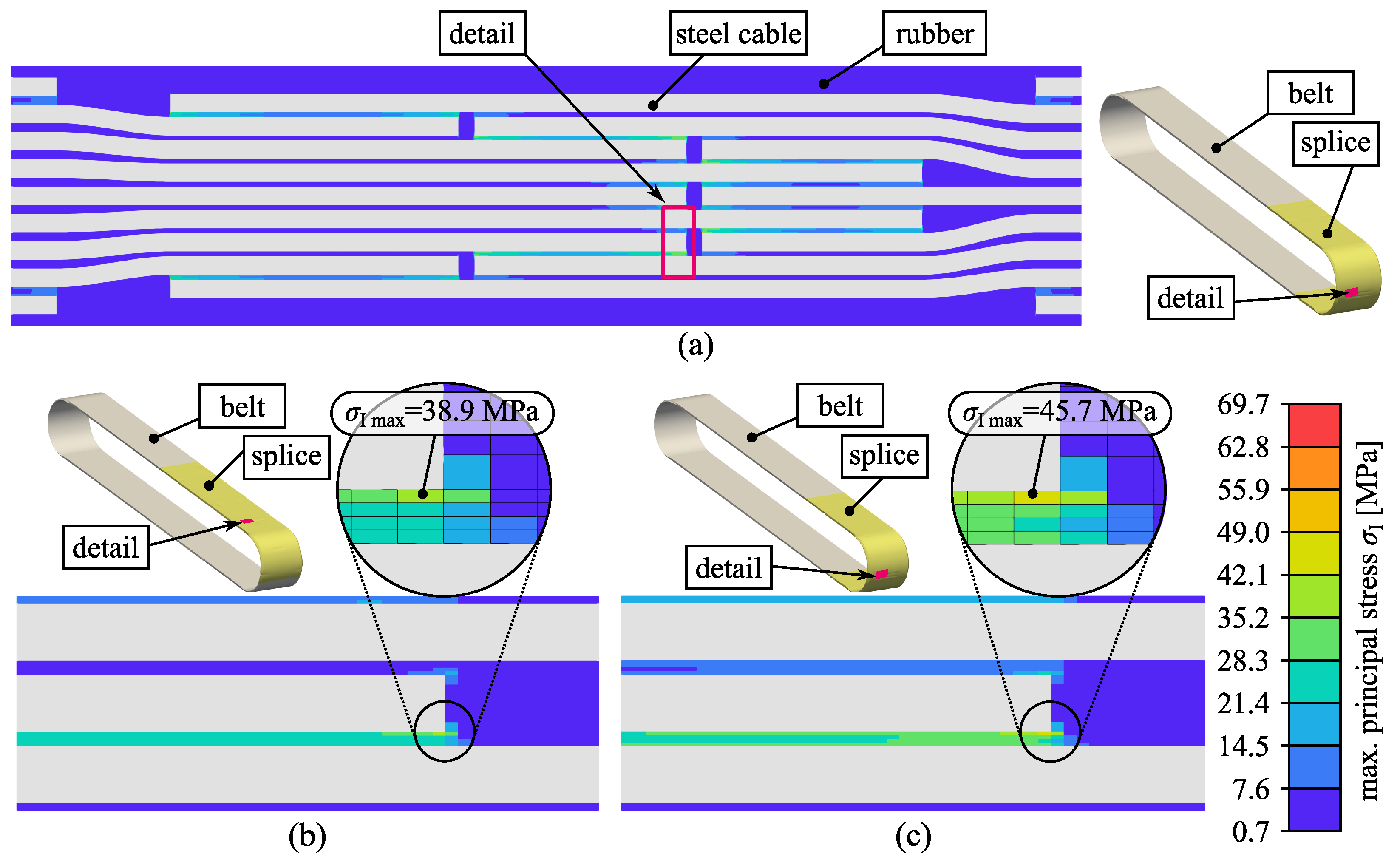
• The region of highest stresses in the used splice scheme occurs at two cable ends due to shear stresses to the neighbouring cables;
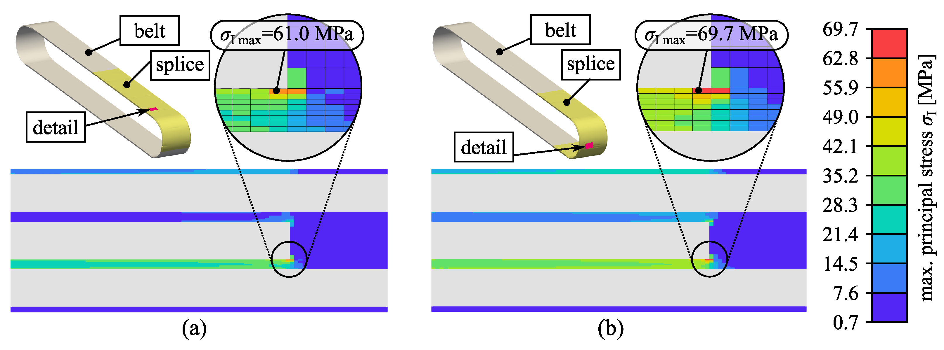
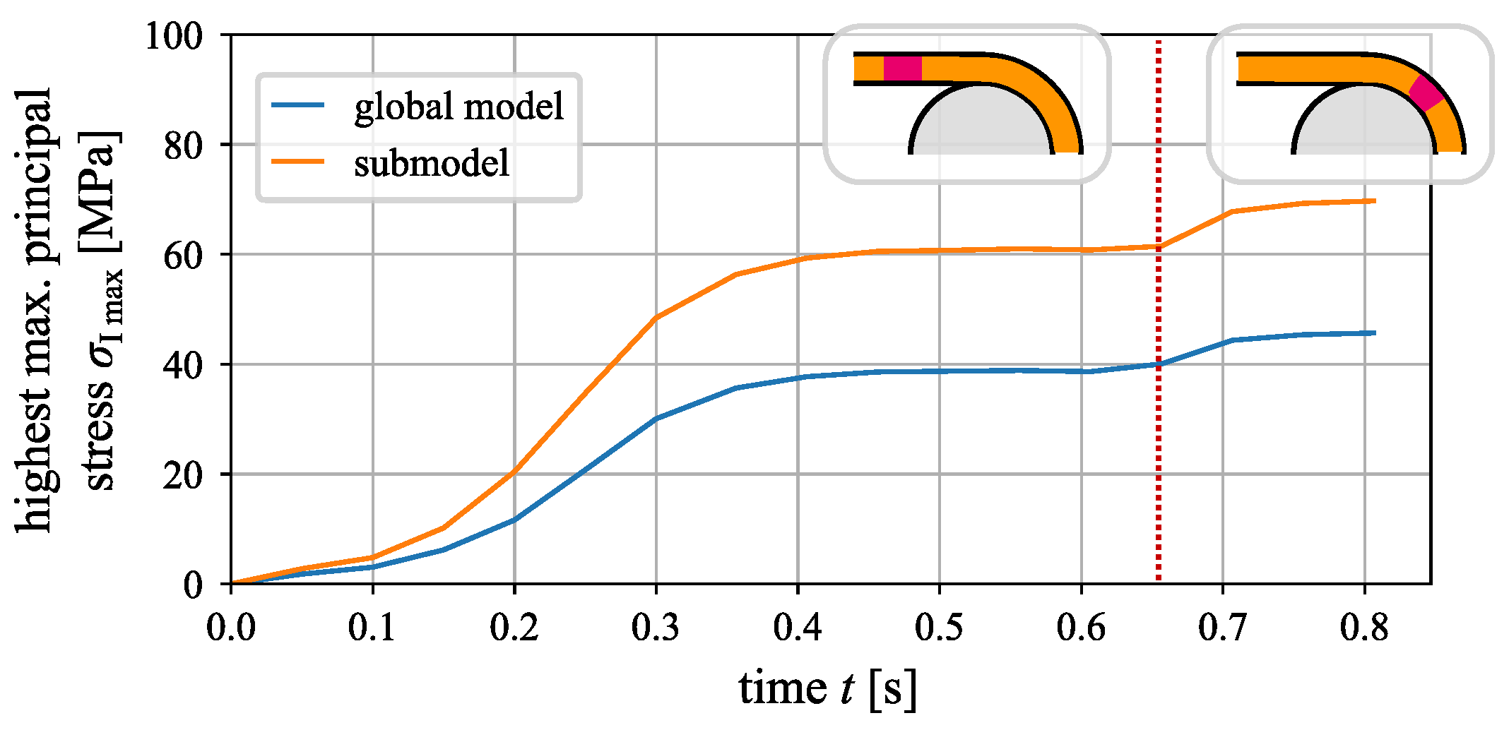
• The test rig model computes by 17.5% higher maximum principal stresses while the critical position of the splice is bent at the drums compared to in the flat region;
• The submodel, where eight instead of four elements are used between the steel cables, computes higher stresses than the global model. The maximum principal stresses reach 14.3% higher values in the bent region than in the flat region.

The developed modelling approach shows a significant influence of bending on the local rubber stresses in the used test rig setup. Therefore, the influence of bending is essential for further fatigue modelling, where accurate stress fields are required. The submodel illustrates how, at a smaller scale, more accurate fracture mechanic concepts such as damage criteria can be used. Other researchers and engineers can benefit from this work by seeing the significance of bending loads on splices and being presented with a modelling approach that can compute this.

References

- DIN 22110-3:2015-04, Prüfverfahren für Fördergurtverbindungen_- Teil_3: Ermittlung der Zeitfestigkeit für Fördergurtverbindungen (Dynamisches Prüfverfahren); Technical Report; Beuth Verlag GmbH: Berlin, Germany, 2015. [CrossRef]
- Kirjanów-Błażej, A.; Jurdziak, L.; Burduk, R.; Błażej, R. Forecast of the remaining lifetime of steel cord conveyor belts based on regression methods in damage analysis identified by subsequent DiagBelt scans. Eng. Fail. Anal. 2019, 100, 119–126. [Google Scholar] [CrossRef]
- Kozłowski, T.; Wodecki, J.; Zimroz, R.; Błażej, R.; Hardygóra, M. A Diagnostics of Conveyor Belt Splices. Appl. Sci. 2020, 10, 6259. [Google Scholar] [CrossRef]
- Fedorko, G.; Molnar, V.; Marasova, D.; Grincova, A.; Dovica, M.; Zivcak, J.; Toth, T.; Husakova, N. Failure analysis of belt conveyor damage caused by the falling material. Part II: Application of computer metrotomography. Eng. Fail. Anal. 2013, 34, 431–442. [Google Scholar] [CrossRef]
- Bonneric, M.; Aubin, V.; Durville, D. Finite element simulation of a steel cable -rubber composite under bending loading: Influence of rubber penetration on the stress distribution in wires. Int. J. Solids Struct. 2019, 160, 158–167. [Google Scholar] [CrossRef] [Green Version]
- Heitzmann, P.; Froböse, T.; Wakatsuki, A.; Overmeyer, L. Optimierung von Textil-Fördergurtverbindungen Mittels Finite Elemente Methode (FEM); Medium: Application/pdf; Wissenschaftliche Gesellschaft für Technische Logistik, Rostock-Warnemünde: Chemnitz, Germany, 2016; Volume 2016. [Google Scholar] [CrossRef]
- Bajda, M.; Błażej, R.; Hardygóra, M. Impact of Selected Parameters on the Fatigue Strength of Splices on Multiply Textile Conveyor Belts. IOP Conf. Ser. Earth Environ. Sci. 2016, 44, 052021. [Google Scholar] [CrossRef]
- Costello, G.A. Theory of Wire Rope; Mechanical Engineering Series; Springer: New York, NY, USA, 1997. [Google Scholar] [CrossRef]
- Nordell, L.; Qiu, X.; Sethi, V. Belt conveyor steel cord splice analysis using finite element methods. Bulk Solids Handl. 1991, 11, 863–868. [Google Scholar]
- Nordell, L. Steel cord belt and splice construction: Modernizing their specifications, improving their economics. Bulk Solids Handl. 1993, 13, 685–693. [Google Scholar]
- Keller, M. Zur Optimierung Hochfester Stahlseilgurtverbindungen. Ph.D. Thesis, Universität Hannover, Hannover, Germany, 2001. [Google Scholar]
- Froböse, T.; Heitzmann, P.; Overmeyer, L.; Wakatsuki, A. Entwicklung eines FE-Modells zur Optimierung von Stahlseil-Fördergurtverbindungen; Medium: Application/pdf; Wissenschaftliche Gesellschaft für Technische Logistik, Rostock-Warnemünde: Chemnitz, Germany, 2014; Volume 2014. [Google Scholar] [CrossRef]
- Froböse, T. Verfahren zur Ermittlung der Materialparameter für die Auslegung von Stahlseil-Fördergurtverbindungen mit Hilfe der FEM; Number 2017, Band 01 in Berichte aus dem ITA; PZH Verlag: Hanover, Germany, 2017. [Google Scholar]
- Li, X.; Long, X.; Shen, Z.; Miao, C. Analysis of Strength Factors of Steel Cord Conveyor Belt Splices Based on the FEM. Adv. Mater. Sci. Eng. 2019, 2019, 1–9. [Google Scholar] [CrossRef] [Green Version]
- Wheatley, G.; Keipour, S. FEA of Conveyor Belt Splice Cord End Conditions. UPB Sci. Bull. Ser. D Mech. Eng. 2021, 83, 205–216. [Google Scholar]
- Li, X.G.; Long, X.Y.; Jiang, H.Q.; Long, H.B. Finite element simulation and experimental verification of steel cord extraction of steel cord conveyor belt splice. In Proceedings of the IOP Conference Series: Materials Science and Engineering, Kitakyushu City, Japan, 10–13 April 2018; Volume 369, p. 012025. [Google Scholar] [CrossRef]
- Carraro, P.; Maragoni, L.; Quaresimin, M. Prediction of the crack density evolution in multidirectional laminates under fatigue loadings. Compos. Sci. Technol. 2017, 145, 24–39. [Google Scholar] [CrossRef]
- Ferdous, W.; Manalo, A.; Yu, P.; Salih, C.; Abousnina, R.; Heyer, T.; Schubel, P. Tensile Fatigue Behavior of Polyester and Vinyl Ester Based GFRP Laminates—A Comparative Evaluation. Polymers 2021, 13, 386. [Google Scholar] [CrossRef] [PubMed]
- ABAQUS Version 2020 User’s Manual; Dassault Systèmes Simulia Corp.: Providence, RI, USA,, 2020.
- Cruz Gómez, M.; Gallardo-Hernández, E.; Vite Torres, M.; Peña Bautista, A. Rubber steel friction in contaminated contacts. Wear 2013, 302, 1421–1425. [Google Scholar] [CrossRef]