
Modeling Stiffness Degradation of Fiber-Reinforced Polymers Based on Crack Densities Observed in Off-Axis Plies


Abstract
:1. Introduction
- The Mori-Tanaka homogenization scheme computes the effect of damage on the stiffness. The resulting stiffness tensor is positive, definite and symmetric. Therefore it meets the thermodynamic limits of the engineering constants of the damaged material without having to develop individual correlations for all the independent engineering constants [29].
- The model can be calibrated easily to a new material. All data to calibrate the model can be obtained with standard static and fatigue tests.
- The stiffness degradation is ply-based. Classical laminate theory is used to compute the overall stiffness of the laminate. Therefore, stress-redistribution to other plies is automatically accounted for. The model builds on well-established methods and focuses on efficiency.
2. Methods
2.1. Experimental Fatigue Data
2.2. Crack Detection
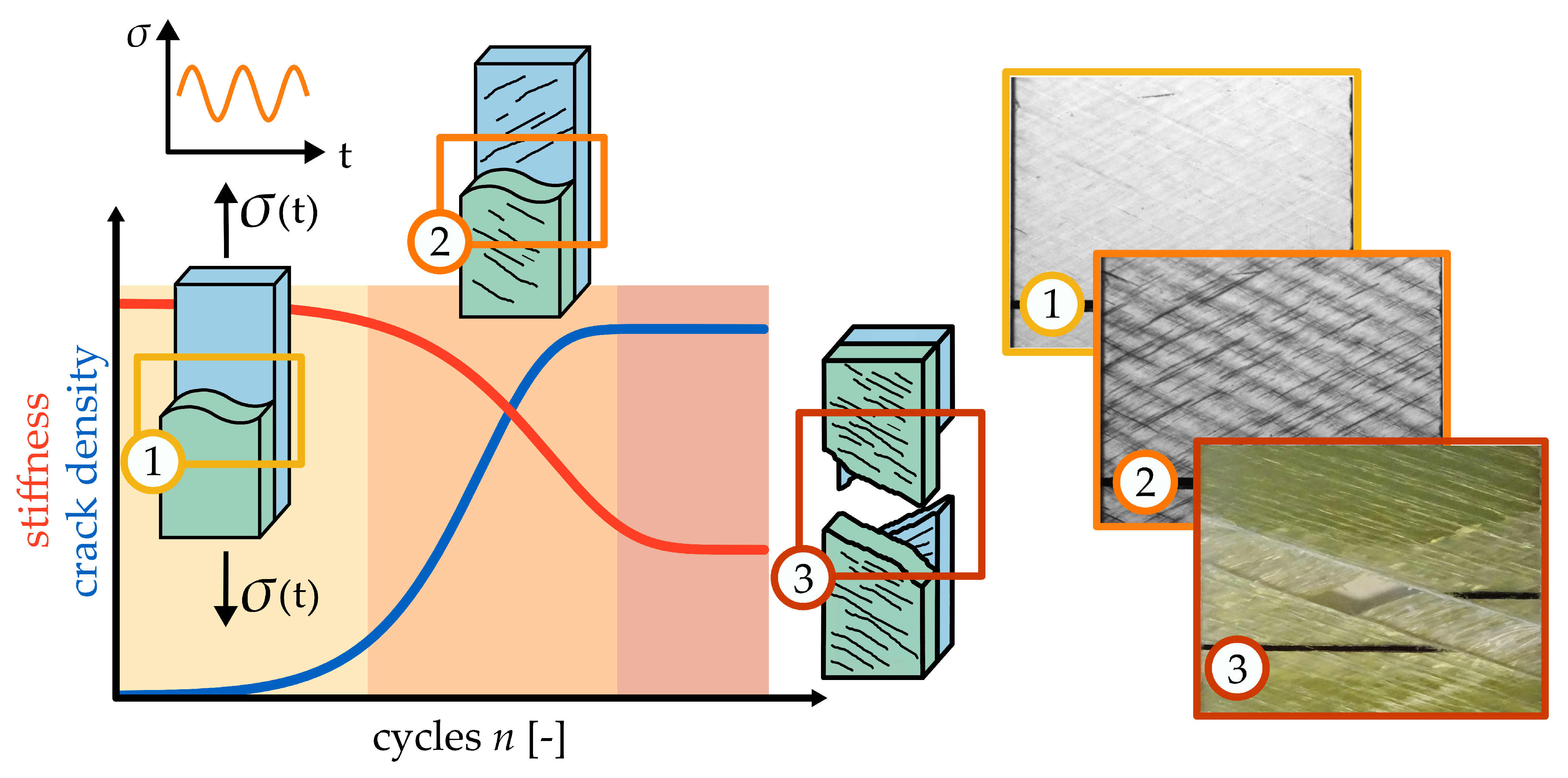
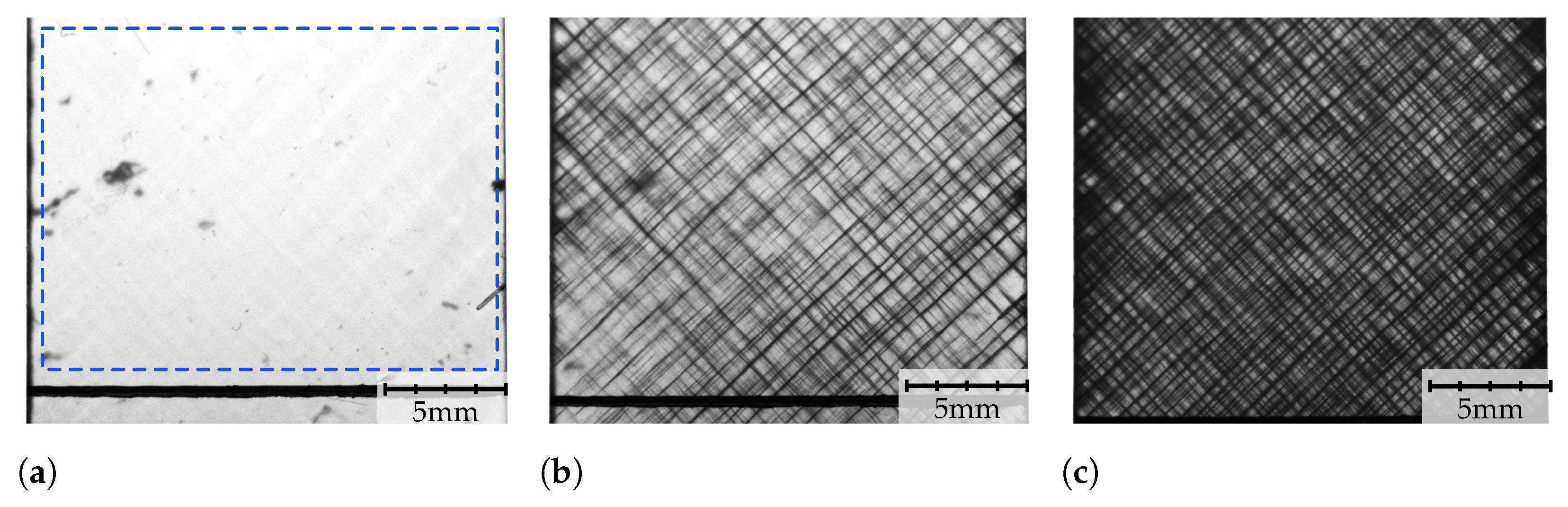
- Shift correction: Since the individual images from a fatigue test are not aligned perfectly due to increasing strain and unavoidable inaccuracies of the test rig (see Figure 2), the shift of the specimen in the images must be corrected.
- Region of interest: Only the area of the specimen without edges or other features like the black line that is used for optical strain measurement (see Figure 2), is evaluated by the crack detection since they might cause false detections.
- Crack detection: Cracks are detected in a cumulative way. Cracks detected in the nth image are added to the n + 1st image.
2.3. Damage Model
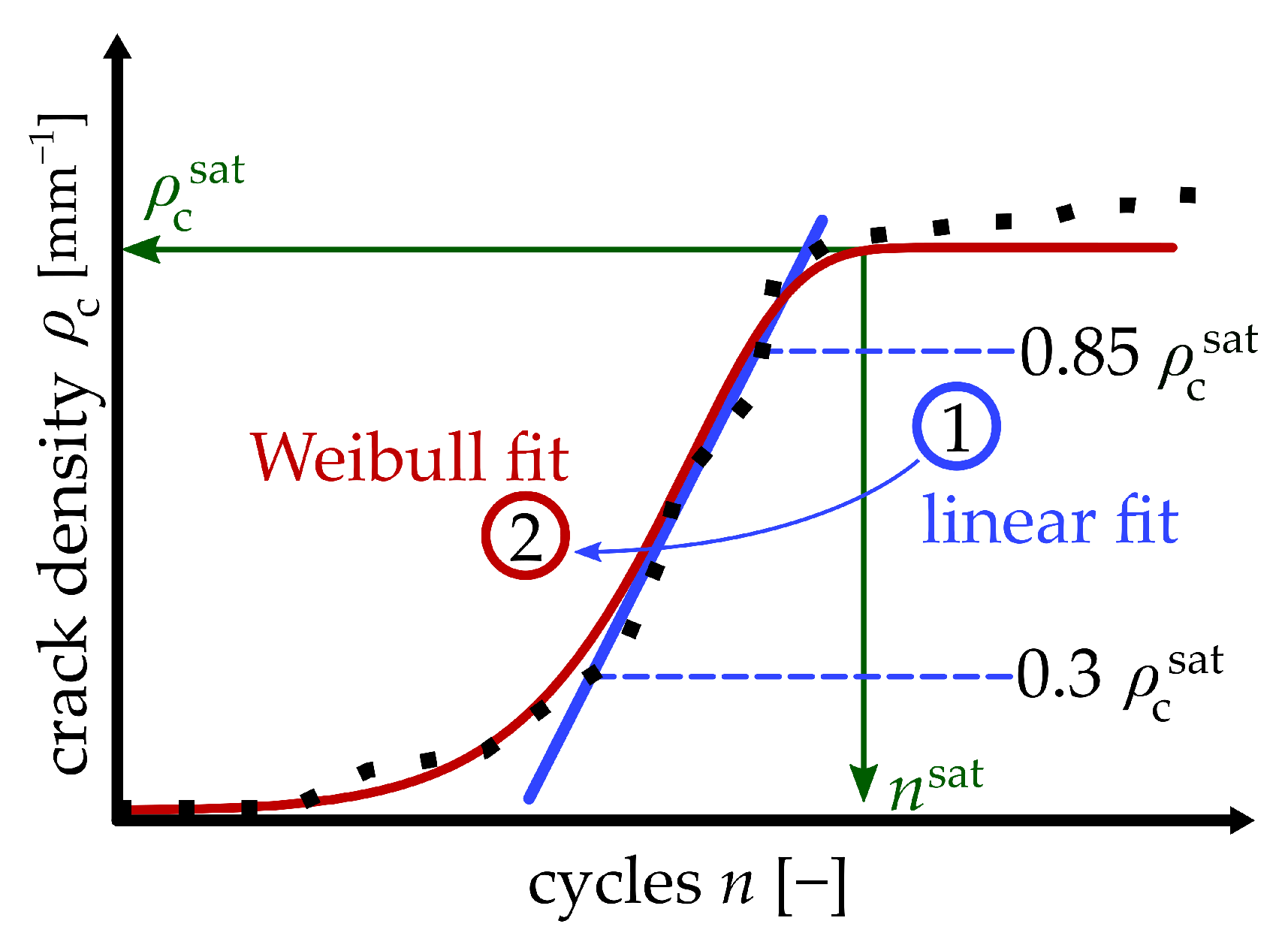
2.4. Calibration
3. Results and Discussion
3.1. Crack Detection Results
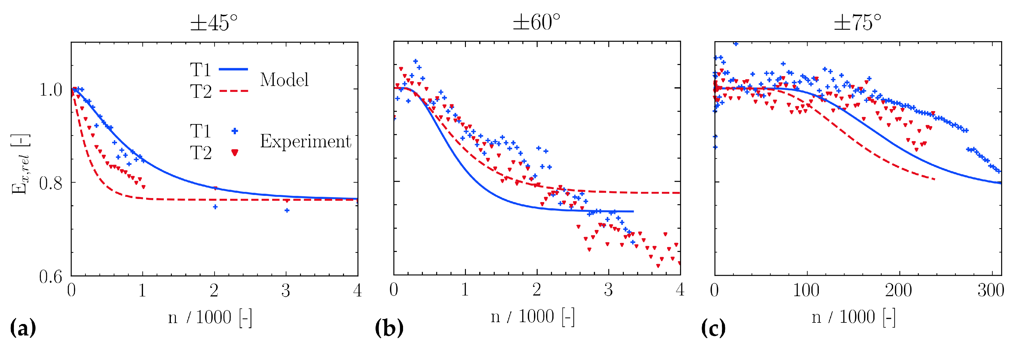
3.2. Stiffness Degradation Model
4. Conclusions
Author Contributions
Funding
Data Availability Statement
Acknowledgments
Conflicts of Interest
Abbreviations
| GFRP | Glass fiber-reinforced polymer |
| TWLI | Transilluminated white light imaging |
| FEM | Finite element method |
| LMPS | Local maximum principal stress |
| LHS | Local hydrostatic stress |
Appendix A. Quasi-Static Material Parameters

| Laminate | Fiber Volume Fraction [−] | Elastic Constant |
|---|---|---|
| 0° | 42.2 | : 33.6 GPa, : 0.28 |
| 90° | 42.4 | : 10.3 GPa |
| ±45° | 52.8 | : 3.7 GPa |
| ±60° | 41.8 | - |
| ±75° | 45.7 | - |
| Matrix | - | : 3.55 GPa, : 0.43 GPa |
Appendix B. Fatigue Load Level

References
- Reifsnider, K.L. (Ed.) Fatigue of Composite Materials; Number 4 in Composite Materials Series; Elsevier: Amsterdam, The Netherlands; New York, NY, USA, 1991. [Google Scholar]
- Tong, J.; Guild, F.J.; Ogin, S.L.; Smith, P.A. Off-axis fatigue crack growth and the associated energy release rate in composite laminates. Appl. Compos. Mater. 1997, 4, 349–359. [Google Scholar] [CrossRef]
- Bartley-Cho, J.; Gyu Lim, S.; Hahn, H.; Shyprykevich, P. Damage accumulation in quasi-isotropic graphite/epoxy laminates under constant-amplitude fatigue and block loading. Compos. Sci. Technol. 1998, 58, 1535–1547. [Google Scholar] [CrossRef]
- Wharmby, A.; Ellyin, F. Damage growth in constrained angle-ply laminates under cyclic loading. Compos. Sci. Technol. 2002, 62, 1239–1247. [Google Scholar] [CrossRef]
- Wharmby, A. Observations on damage development in fibre reinforced polymer laminates under cyclic loading. Int. J. Fatigue 2003, 25, 437–446. [Google Scholar] [CrossRef]
- Tohgo, K.; Nakagawa, S.; Kageyama, K. Fatigue behavior of CFRP cross-ply laminates under on-axis and off-axis cyclic loading. Int. J. Fatigue 2006, 28, 1254–1262. [Google Scholar] [CrossRef]
- Quaresimin, M.; Carraro, P. Damage initiation and evolution in glass/epoxy tubes subjected to combined tension–torsion fatigue loading. Int. J. Fatigue 2014, 63, 25–35. [Google Scholar] [CrossRef]
- Shen, H.; Yao, W.; Qi, W.; Zong, J. Experimental investigation on damage evolution in cross-ply laminates subjected to quasi-static and fatigue loading. Compos. Part B Eng. 2017, 120, 10–26. [Google Scholar] [CrossRef]
- Carraro, P.; Quaresimin, M. A stiffness degradation model for cracked multidirectional laminates with cracks in multiple layers. Int. J. Solids Struct. 2015, 58, 34–51. [Google Scholar] [CrossRef]
- Glud, J.; Dulieu-Barton, J.; Thomsen, O.; Overgaard, L. Fatigue damage evolution in GFRP laminates with constrained off-axis plies. Compos. Part A Appl. Sci. Manuf. 2017, 95, 359–369. [Google Scholar] [CrossRef] [Green Version]
- Zhang, D.; Ye, J.; Lam, D. Ply cracking and stiffness degradation in cross-ply laminates under biaxial extension, bending and thermal loading. Compos. Struct. 2006, 75, 121–131. [Google Scholar] [CrossRef]
- Thionnet, A.; Renard, J. Laminated composites under fatigue loading: A damage development law for transverse cracking. Compos. Sci. Technol. 1994, 52, 173–181. [Google Scholar] [CrossRef]
- Nuismer, R.J.; Tan, S.C. Constitutive Relations of a Cracked Composite Lamina. J.Compos.Mater. 1988, 22, 306–321. [Google Scholar] [CrossRef]
- Varna, J. Modelling mechanical performance of damaged laminates. J. Compos. Mater. 2013, 47, 2443–2474. [Google Scholar] [CrossRef]
- Joffe, R.; Varna, J. Analytical modeling of stiffness reduction in symmetric and balanced laminates due to cracks in 90° layers. Compos. Sci. Technol. 1999, 59, 1641–1652. [Google Scholar] [CrossRef]
- Jagannathan, N.; Gururaja, S.; Manjunatha, C. Probabilistic strength based matrix crack evolution model in multi-directional composite laminates under fatigue loading. Int. J. Fatigue 2018, 117, 135–147. [Google Scholar] [CrossRef]
- Singh, C.V.; Talreja, R. A synergistic damage mechanics approach for composite laminates with matrix cracks in multiple orientations. Mech. Mater. 2009, 41, 954–968. [Google Scholar] [CrossRef]
- Quaresimin, M.; Carraro, P. On the investigation of the biaxial fatigue behaviour of unidirectional composites. Compos. Part B Eng. 2013, 54, 200–208. [Google Scholar] [CrossRef]
- Adden, S.; Horst, P. Stiffness degradation under fatigue in multiaxially loaded non-crimped-fabrics. Int. J. Fatigue 2010, 32, 108–122. [Google Scholar] [CrossRef]
- Jespersen, K.M.; Glud, J.A.; Zangenberg, J.; Hosoi, A.; Kawada, H.; Mikkelsen, L.P. Uncovering the fatigue damage initiation and progression in uni-directional non-crimp fabric reinforced polyester composite. Compos. Part A Appl. Sci. Manuf. 2018, 109, 481–497. [Google Scholar] [CrossRef] [Green Version]
- Sket, F.; Enfedaque, A.; Alton, C.; González, C.; Molina-Aldareguia, J.; Llorca, J. Automatic quantification of matrix cracking and fiber rotation by X-ray computed tomography in shear-deformed carbon fiber-reinforced laminates. Compos. Sci. Technol. 2014, 90, 129–138. [Google Scholar] [CrossRef] [Green Version]
- Sørensen, B.F.; Talreja, R. Analysis of Damage in a Ceramic Matrix Composite. Int. J. Damage Mech. 1993, 2, 246–271. [Google Scholar] [CrossRef]
- Lafarie-Frenot, M.; Hénaff-Gardin, C. Formation and growth of 90° ply fatigue cracks in carbon/epoxy laminates. Compos. Sci. Technol. 1991, 40, 307–324. [Google Scholar] [CrossRef]
- Glud, J.; Dulieu-Barton, J.; Thomsen, O.; Overgaard, L. Automated counting of off-axis tunnelling cracks using digital image processing. Compos. Sci. Technol. 2016, 125, 80–89. [Google Scholar] [CrossRef] [Green Version]
- Drvoderic, M.; Rettl, M.; Pletz, M.; Schuecker, C. CrackDect: Detecting crack densities in images of fiber-reinforced polymers. SoftwareX 2021, 16, 100832. [Google Scholar] [CrossRef]
- Degrieck, J.; Van Paepegem, W. Fatigue damage modeling of fibre-reinforced composite materials: Review. Appl. Mech. Rev. 2001, 54, 279–300. [Google Scholar] [CrossRef]
- Schuecker, C.; Pettermann, H. A continuum damage model for fiber reinforced laminates based on ply failure mechanisms. Compos. Struct. 2006, 76, 162–173. [Google Scholar] [CrossRef]
- Mori, T.; Tanaka, K. Average stress in matrix and average elastic energy of materials with misfitting inclusions. Acta Metall. 1973, 21, 571–574. [Google Scholar] [CrossRef]
- Benveniste, Y.; Dvorak, G.; Chen, T. On diagonal and elastic symmetry of the approximate effective stiffness tensor of heterogeneous media. J. Mech. Phys. Solids 1991, 39, 927–946. [Google Scholar] [CrossRef]
- Schuecker, C.; Pettermann, H. Constitutive ply damage modeling, FEM implementation, and analyses of laminated structures. Comput. Struct. 2008, 86, 908–918. [Google Scholar] [CrossRef]
- Carraro, P.; Maragoni, L.; Quaresimin, M. Prediction of the crack density evolution in multidirectional laminates under fatigue loadings. Compos. Sci. Technol. 2017, 145, 24–39. [Google Scholar] [CrossRef]
- Rieser, R. Damage Mechanics of Composites under Fatigue Loads. Ph.D. Thesis, Montanuniversität Leoben, Leoben, Austria, 2016. [Google Scholar]
- Puck, A. Failure analysis of FRP laminates by means of physically based phenomenological models. Compos. Sci. Technol. 2002, 62, 1633–1662. [Google Scholar] [CrossRef]
- SciPy 1.0 Contributors; Virtanen, P.; Gommers, R.; Oliphant, T.E.; Haberland, M.; Reddy, T.; Cournapeau, D.; Burovski, E.; Peterson, P.; Weckesser, W.; et al. SciPy 1.0: Fundamental algorithms for scientific computing in Python. Nat. Methods 2020, 17, 261–272. [Google Scholar] [CrossRef] [Green Version]
- Eshelby, J.D. The determination of the elastic field of an ellipsoidal inclusion, and related problems. Proc. R. Soc. London Ser. Math. Phys. Sci. 1957, 241, 376–396. [Google Scholar] [CrossRef]
- Parnell, W.J. The Eshelby, Hill, Moment and Concentration Tensors for Ellipsoidal Inhomogeneities in the Newtonian Potential Problem and Linear Elastostatics. J. Elast. 2016, 125, 231–294. [Google Scholar] [CrossRef]
- Gavazzi, A.C.; Lagoudas, D.C. On the numerical evaluation of Eshelby’s tensor and its application to elastoplastic fibrous composites. Comput. Mech. 1990, 7, 13–19. [Google Scholar] [CrossRef]
- Miskdjian, I.; Hajikazemi, M.; Van Paepegem, W. Automatic edge detection of ply cracks in glass fiber composite laminates under quasi-static and fatigue loading using multi-scale Digital Image Correlation. Compos. Sci. Technol. 2020, 200, 108401. [Google Scholar] [CrossRef]
- Vasylevskyi, K.; Drach, B.; Tsukrov, I. On micromechanical modeling of orthotropic solids with parallel cracks. Int. J. Solids Struct. 2018, 144–145, 46–58. [Google Scholar] [CrossRef]
- Drach, B.; Tsukrov, I.; Trofimov, A. Comparison of full field and single pore approaches to homogenization of linearly elastic materials with pores of regular and irregular shapes. Int. J. Solids Struct. 2016, 96, 48–63. [Google Scholar] [CrossRef]
- Seabold, S.; Perktold, J. Statsmodels: Econometric and Statistical Modeling with Python. In Proceedings of the 9th Python in Science Conference, Austin, TX, USA, 28 June– 3 July 2010; pp. 92–96. [Google Scholar] [CrossRef] [Green Version]
- Carraro, P.; Quaresimin, M. A damage based model for crack initiation in unidirectional composites under multiaxial cyclic loading. Compos. Sci. Technol. 2014, 99, 154–163. [Google Scholar] [CrossRef]
- Plumtree, A. Fatigue damage evolution in off-axis unidirectional CFRP. Int. J. Fatigue 2002, 24, 155–159. [Google Scholar] [CrossRef]
- Younes, R.; Hallal, A.; Fardoun, F.; Hajj, F. Comparative Review Study on Elastic Properties Modeling for Unidirectional Composite Materials. In Composites and Their Properties; Hu, N., Ed.; InTech: London, UK, 2012. [Google Scholar] [CrossRef] [Green Version]


| [GPa] | [GPa] | [−] | [GPa] | [MPa] | [MPa] |
|---|---|---|---|---|---|
| 35.6 | 10.9 | 0.27 | 3.2 | 57.9 | 58.3 |
| Test | Ply Angle [] | Crack Width [px] | Pixel per mm | ||||
|---|---|---|---|---|---|---|---|
| ±45° T1 | 45 | 8 | 69.2 | 200 | 1500 | 0 | 900 |
| ±45° T2 | 45 | 8 | 70.3 | 200 | 1500 | 0 | 950 |
| ±60° T1 | 60 | 8 | 68.8 | 100 | 1400 | 0 | 850 |
| ±60° T2 | 60 | 10 | 70.2 | 100 | 1400 | 0 | 1000 |
| ±75° T1 | 75 | 15 | 69.6 | 200 | 1400 | 0 | 1000 |
| ±75° T2 | 75 | 12 | 70.2 | 200 | 1450 | 0 | 900 |
| Test | [] | [] | ||
|---|---|---|---|---|
| ±45° T1 | 3 | 140 | 4000 | 2.8 |
| ±45° T2 | 3 | 30 | 1500 | 2.7 |
| ±60° T1 | 2.1 | 304 | 2100 | 3.2 |
| ±60° T2 | 1.7 | 487 | 2200 | 2.3 |
| ±75° T1 | 1.3 | 93,086 | - | 2.9 |
| ±75° T2 | 1.3 | 68,314 | - | 2.7 |
Publisher’s Note: MDPI stays neutral with regard to jurisdictional claims in published maps and institutional affiliations. |
© 2021 by the authors. Licensee MDPI, Basel, Switzerland. This article is an open access article distributed under the terms and conditions of the Creative Commons Attribution (CC BY) license (https://creativecommons.org/licenses/by/4.0/).
Share and Cite
Drvoderic, M.; Pletz, M.; Schuecker, C. Modeling Stiffness Degradation of Fiber-Reinforced Polymers Based on Crack Densities Observed in Off-Axis Plies. J. Compos. Sci. 2022, 6, 10. https://doi.org/10.3390/jcs6010010
Drvoderic M, Pletz M, Schuecker C. Modeling Stiffness Degradation of Fiber-Reinforced Polymers Based on Crack Densities Observed in Off-Axis Plies. Journal of Composites Science. 2022; 6(1):10. https://doi.org/10.3390/jcs6010010
Chicago/Turabian StyleDrvoderic, Matthias, Martin Pletz, and Clara Schuecker. 2022. "Modeling Stiffness Degradation of Fiber-Reinforced Polymers Based on Crack Densities Observed in Off-Axis Plies" Journal of Composites Science 6, no. 1: 10. https://doi.org/10.3390/jcs6010010
APA StyleDrvoderic, M., Pletz, M., & Schuecker, C. (2022). Modeling Stiffness Degradation of Fiber-Reinforced Polymers Based on Crack Densities Observed in Off-Axis Plies. Journal of Composites Science, 6(1), 10. https://doi.org/10.3390/jcs6010010