Numerical Study of Soil-Thawing Effect of Composite Piles Using GMsFEM

Abstract

During construction works, it is advisable to prevent strong thawing and an increase in the moisture content of the foundations of engineering structures in the summer. Since the density of water and ice differ, due to the difference bulging of the foundation sections can occur when it freezes back in winter. In this work, the effect of fiber-reinforced piles on the thermal field of the surrounding soil is investigated numerically; that is, the study of the influence of aggregates with high and low thermal-physical properties on the temperature of frozen soils is conducted. Basalt and steel fiber reinforcement are compared. The difficulty of this work is that the inclusions inside piles are too small compared to the pile itself. Therefore, to solve the Stefan problem, a generalized multiscale finite element method (GMsFEM) was used. In the GMsFEM, the usual conforming partition of the domain into a coarse grid was used. It allowed reducing problem size and, consequently, accelerating the calculations. Results of the multiscale solution were compared with fine-scale solution, the accuracy of GMsFEM was investigated, and the optimal solution parameters were defined. Therefore, GMsFEM was shown to be well suited for the designated task. Collation of basalt and steel fiber reinforcement showed a beneficial effect of high thermal conductive material inclusion on freezing of piles in winter.

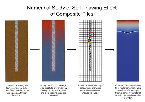
1. Introduction

Thermal calculations are important in the construction of engineering geotechnical structures and buildings in the permafrost zone. The temperature regime (a set of sequential temperature fields in the soil mass corresponding to any given points in time from the beginning of the calculation) is calculated as the forecast of the thermal effects on the upper and lower boundaries of the structure foundation set for the entire calculation period [1]. The most characteristic feature of these processes is the previously unknown (“free”) boundaries between various thawed and frozen states of the soil. Due to this feature, their mathematical models are non-linear and difficult to analyze. The results of calculations of climatic phenomena, which are critical for geotechnical structures on permafrost foundations (in the permafrost zone), show a continuous repetition of the same constant seasonal cycle. This determines periodic harmonic oscillations of all quantities that determine the state of the foundation of a geotechnical structure, including temperature. However, cyclic harmonic changes in the foundation state caused by constantly repeating influences also occur during other processes. The course of temperature change during one period can have a different character. For example, the temperature can change abruptly, continuously increase or decrease, etc.

During construction works, it is advisable to prevent strong thawing and an increase in the moisture content of the foundations of engineering structures in the summer. Since the density of water and ice differ, due to the difference bulging of the foundation sections can occur when it freezes back in winter. Repetition of this phenomenon for many years causes the destruction of engineering structures and buildings. In the regions of the Far North, it leads to catastrophic emergencies.

In this work, the effect of fiber-reinforced piles on the thermal field of the surrounding soil is numerically investigated [2], that is, the study of the influence of aggregates with high and low thermal-physical properties on the temperature of frozen soils is conducted [3,4].

Basalt fibers are produced from molten basalt rock. They have very low thermal conductivity, good strength properties and, at the same time, are relatively cheap. Due to these characteristics, they are used in concrete [5,6,7]. However, in addition to the chemical and mechanical properties of basalt fibers, their cost varies, depending on the type and quality of the raw material and the production process of these fibers [8]. Nevertheless, the characteristics mentioned above and an environmentally friendly manufacturing process [9] might determine their application in high performance concrete structures instead of the most commonly used steel and polypropylene fibers. The length-to-diameter aspect for basalt fibers is about 1000.

As for steel fiber hybridization, industrial or recycled steel fibers can be used [10,11,12,13]. According to results available in the scientific literature [14,15], they show similar mechanical responses, both in terms of tensile strength and matrix-to-fiber bond. Recycled steel fibers are derived from waste tires. Their geometrical characterization can be highly variable: they are generally characterized by a nominal diameter ranging between 0.1 and 2 mm with a corresponding average aspect ratio (i.e., length-to-diameter ratio) ranging between 20 and 150. These variations mainly depend on both the original source (i.e., tires typology) and recycling processes.

The volume concentration of fibers is equal to 10%. In our article, we use the length-to-diameter ratio for both types of fibers equal to 32 for structured and 10 for random distribution of fibers for calculation convenience. Fibers’ mechanical properties are presented in

Table 1. Mechanical properties of fibers.

Fiber Type	Steel	Basalt
Density (kg/m3)	7800	2700
Volume content (kg/m3)	780	270
Elastic modulus (GPa)	200	70
Tensile strength (MPa)	>1060	>1700

.

One of the topical problems of mathematical physics is the Stefan problem, which is an initial–boundary value problem for a parabolic differential equation with discontinuous coefficients, and serves as a mathematical model of the change in the phase state of a substance with unknown interfaces [16,17]. The phase transition boundary is represented as a smearing zone when the phase transition occurs in a given temperature range [16,18].

The difficulty of this work lies in the pile inclusions that are too small compared to the solution area. For such geometrically complex problems, reduction techniques such as multiscale methods are preferred [19,20]. Multiscale methods are becoming very popular at this time [21,22,23]. Paper [24] develops a multiscale eigenvalue method based on multiscale substructure technology for multiscale analysis of periodic composite structures. This provides a comparative study from a user’s viewpoint for multiscale methods, including the mathematical homogenization method, heterogeneous multiscale method, and multiscale finite element method. The article [25] studies the multiscale finite element method for solving elliptic problems arising from composite materials. The influence of production porosity, diameter [26], and density of structures on the thermal conductivity of a composite are considered using multiscale finite element modeling [27]. In [28,29], mathematical modeling is applied for the thermodynamic analysis and design of composite structures.

This article is organized as follows. Section 2 presents the formulation of a mathematical model that describes the dynamics of the temperature distribution with the phase transitions taken into account. In the third, finite element approximation is given. In the fourth, a generalized multiscale finite element method (GMsFEM) is considered. Section 5 presents the numerical results in a two-dimensional setting.

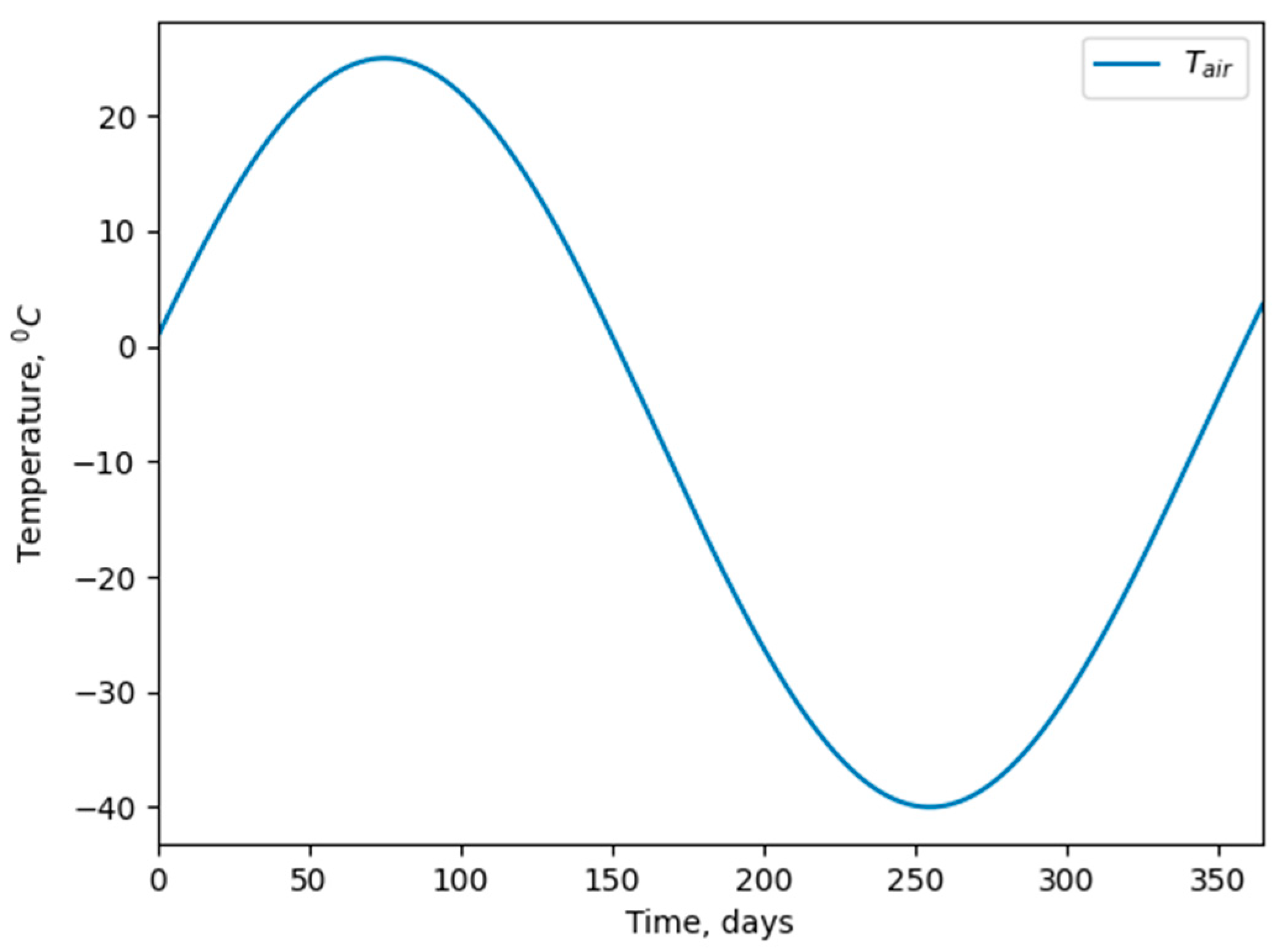
2. Mathematical Model

Let us consider a mathematical model describing the dynamics of the temperature distribution, taking into account the phase transitions of pore moisture into ice and back, at a certain given temperature of the phase transition $T^{*}$ in area $\mathsf{\Omega }={\mathsf{\Omega }}^{-}{\displaystyle \cup }{\mathsf{\Omega }}^{+}$. Where ${\mathsf{\Omega }}^{+}\left(t\right)=\left\{x|x\in \mathsf{\Omega }, T\left(x,t\right)>T\right\}$ is the area occupied by the thawed soil, where the temperature exceeds the phase transition temperature and ${\mathsf{\Omega }}^{-}\left(t\right)=\left\{x\right|x\in \mathsf{\Omega }, T\left(x,t\right)<T\}$ is an area occupied by the frozen ground. A phase transition occurs at the interface between thawed and frozen soils $S=S\left(t\right)$ (Figure 1).

To simulate heat transfer processes with phase transitions, the Stefan model is used. It describes thermal processes accompanying phase transformations of the medium with absorption and release of latent heat:

$$\left(c\rho \left(T\right)+m{\rho }_{l}L\delta \left(T-T^{*}\right)\right)\frac{\partial T}{\partial t}-\mathrm{div}\left(\lambda \left(T\right)T\right)=f,\hspace{1em}x\in \mathsf{\Omega },\hspace{1em}t\in \left(0,t_{max}\right],$$

(1)

where $L$ is the specific heat of phase transition, m is a porosity, $\delta \left(T-T^{*}\right)$ is Dirac delta function.

For the coefficients of the equation, there are following relations:

$$c\rho \left(T\right)=\{\begin{array}{c}{c}^{-}{\rho }^{-}, T<T^{*},\\ c^{+}{\rho }^{+}, T\ge T^{*},\end{array}\hspace{1em}\lambda \left(T\right)=\{\begin{array}{c}{\lambda }^{-}, T<T^{*},\\ {\lambda }^{+}, T\ge T^{*},\end{array}$$

where $c^{+}, {\rho }^{+},{\lambda }^{+}$ and $c^{-}, {\rho }^{-},{\lambda }^{-}$ are the specific heat, density, and thermal conductivity of thawed and frozen soil, respectively.

Since the process of heat propagation is considered in a saturated porous medium, there are following thermal-physical characteristics:

$$c^{-}{\rho }^{-}=\left(1-m\right)c_{sc}{\rho }_{sc}+m{c}_i{\rho }_i,\hspace{1em}{c}^{+}{\rho }^{+}=\left(1-m\right)c_{sc}{\rho }_{sc}+m{c}_w{\rho }_w,$$

where $m$ is a porosity. The subscripts $sc, w, i$ denote the skeleton of the porous medium, water, and ice, respectively. For the coefficients of the thermal conductivity in the thawed and frozen zones, there are similar relations:

$${\lambda }^{-}=\left(1-m\right){\lambda }_{sc}+m{\lambda }_i,\hspace{1em}{\lambda }^{+}=\left(1-m\right){\lambda }_{sc}+m{\lambda }_w,$$

In practice, phase transformations do not take place instantly and can proceed in a small temperature range $\left[T-\mathsf{\Delta }, T+\mathsf{\Delta }\right]$. The discontinuous coefficients of Equation (1) are replaced by sufficiently smooth functions of temperature:

$${\left(c\rho \right)}_{\mathsf{\Delta }}\left(T\right)=c^{-}{\rho }^{-}+m\left(c^{+}{\rho }^{+}-c^{-}{\rho }^{-}\right)\frac{1}{2}\left(1+\mathrm{erf}\left(\frac{T-T^{*}}{\sqrt{2{\mathsf{\Delta }}^2}}\right)\right)+\frac{1}{\sqrt{2\pi {\mathsf{\Delta }}^2}}{e}^{-\frac{{\left(T-T^{*}\right)}^2}{2{\mathsf{\Delta }}^2}},$$

$${\lambda }_{\mathsf{\Delta }}\left(T\right)={\lambda }^{-}+m\left({\lambda }^{+}-{\lambda }^{-}\right)\frac{1}{2}\left(1+\mathrm{erf}\left(\frac{T-T^{*}}{\sqrt{2{\mathsf{\Delta }}^2}}\right)\right).$$

Thus, the following equation for the temperature is obtained:

$${\left(c\rho \right)}_{\mathsf{\Delta }}\left(T\right)\frac{\partial T}{\partial t}-\mathrm{div}\left({\lambda }_{\mathsf{\Delta }}\left(T\right)T\right)=f,\hspace{1em}x\in \mathsf{\Omega },\hspace{1em}t\in \left(0,t_{max}\right],$$

(2)

Thus, Equation (2) is a multidimensional quasilinear parabolic equation with smooth coefficients.

For piles and fibers the following is true: ${\left(c\rho \right)}_{\mathsf{\Delta }}={\left(c\rho \right)}_{p,f}$ and ${\lambda }_{\mathsf{\Delta }}={\lambda }_{\mathrm{p},\mathrm{f}}$, where $c_{p,f},{\rho }_{p,f},{\lambda }_{\mathrm{p},\mathrm{f}}$ are specific heat, density, and thermal conductivity of piles and fibers. That is, there is no phase transition in the pile and fiber areas, respectively.

Equation (2) is supplemented with the initial and boundary conditions

$$T\left(x,0\right)=T_0,$$

$$-\lambda \frac{\partial T}{\partial \eta }=\alpha \left(T-T_{air}\right), x\in {\mathsf{\Gamma }}_t,$$

$$-\lambda \frac{\partial T}{\partial \eta }=0, x\in \frac{\mathsf{\Gamma }}{{\mathsf{\Gamma }}_t}.$$

Here $\eta$—normal vector.

3. Fine-Scale Approximation

The quasilinear parabolic Equation (2) with the corresponding boundary and initial conditions is approximated using the finite element method in combination with a purely implicit linearized finite difference approximation in time. This means that during discretization, the coefficients depending on the desired function are taken from the previous time layer. Let us write down the variational problem statement for each time layer: find $T\in H^1$ such that:

$$a\left(T^{n+1},v\right)=L\left(v\right), \forall \in H_0^1,$$

where

$$\begin{array}{l}a\left(T^{n+1},v\right) = \frac{1}{\tau }{{\displaystyle \int }}_{\mathsf{\Omega }}{\left(c\rho \right)}_{\sigma }(T^n)T^{n+1}wdx + {{\displaystyle \int }}_{\mathsf{\Omega }}{\lambda }_{\sigma }(T^n)T^{n+1}·wdx + {{\displaystyle \int }}_{\Gamma t}\alpha T^{n+1}ds,\\ L(v) = \frac{1}{\tau }{{\displaystyle \int }}_{\mathsf{\Omega }}{\left(c\rho \right)}_{\sigma }{T}^{n}wdx + {{\displaystyle \int }}_{\Gamma t}\alpha T_{air}ds.\end{array}$$

To solve the problem numerically, it is necessary to pass from a continuous variational problem to a discrete one. For this, finite-dimensional spaces V_h ∈ H¹, ${\widehat{V}}_h\in H_0^1$ are introduced and the following problem is defined on them: find $T_h\in V_h$ such that:

$$a\left(T_h^{n+1},v\right)=L\left(v\right), \forall \in {\widehat{V}}_h,$$

where

$$\begin{array}{l}a\left(T^{n+1},v\right) = \frac{1}{\tau }{{\displaystyle \int }}_{\mathsf{\Omega }}{\left(c\rho \right)}_{\sigma }(T^n)T^{n+1}{w}_{h}dx + {{\displaystyle \int }}_{\mathsf{\Omega }}{\lambda }_{\sigma }(T^n)T_h^{n+1}·w_{h}dx + {{\displaystyle \int }}_{\Gamma t}\alpha T^{n+1}ds,\\ L(v) = \frac{1}{\tau }{{\displaystyle \int }}_{\mathsf{\Omega }}{\left(c\rho \right)}_{\sigma }{T}_h^n{w}_{h}dx + {{\displaystyle \int }}_{\Gamma t}\alpha T_{air}ds.\end{array}$$

4. Generalized Multiscale Finite Element Method (GMsFEM)

Construction local reduction of a model on the snapshot space is described by solving several local spectral problems using GMsFEM. In the GMsFEM the usual conforming partition of domain into finite elements is used. This partition is called the coarse grid ${\mathcal{T}}_H$. The coarse grid is partitioned into coarse-grid blocks. That is, ${\mathcal{T}}_H$ is a coarse grid in domain Ω, such that ${\mathcal{T}}_H={{\displaystyle \cup }}_{i=1}^{N_c}{K}_i$, where K_i is coarse cell. The ${\mathcal{T}}_h$ is a fine grid with $H\ge h\ge 0$, where $h$ is size of fine grid. Each coarse-grid block ($K_i$) consists of the connected union of fine-grid blocks. Furthermore, a certain domain for this is constructed and denoted by $N_c$ the coarse nodes number, by ${\left\{x_i\right\}}_{i=1}^{N_c}$ the vertices of the coarse mesh and define the neighborhood of the node $x_i$:

$${\omega }_i={\displaystyle \cup }\left\{K_i\in {\mathcal{T}}_H;\hspace{1em}{x}_i\in \overline{K_i}\right\}$$

The following steps need to be implemented for GMsFEM realization:

• Coarse grid generation ${\mathcal{T}}_H;$
• Offline space construction;
• Construction of snapshot space that will be used to compute an offline space;
• Construction of a small dimensional offline space by performing dimensional reduction in the space of local snapshots;
• Solution of a coarse-grid problem for any force term and boundary condition.

In the first step of GMsFEM (Offline stage), the “snapshots” space must be constructed, a large dimensional snapshots space of local solutions. In the “snapshots” space, the following is considered:

$$-\mathrm{div}\left(k_{\alpha }\nabla {\psi }_j\right)=0,\hspace{1em}x\in {\omega }_i,$$

$${\psi }_j={\delta }_j\left(x\right),\hspace{1em}x\in \partial {\omega }_i,$$

where $k_{\alpha }$ are the coefficients of the thermal conductivity, ${\delta }_j\left(x\right)$ are certain set of function defined on $\partial {\omega }_i$, here $j=1, J_{\omega }$. The $J_{\omega }$ is a number of fine grid edges on $\omega$. Therefore, following is defined:

$$V_{\mathrm{snap}}=\mathrm{span}\{{\psi }_j^{\mathrm{snap}}: 1\le \mathrm{j}\le J_{\omega }\}, \mathrm{and} R_{\mathrm{snap}}=\left[{\psi }_1^{\mathrm{snap}},\dots ,{\psi }_{J_{\omega }}^{\mathrm{snap}}\right]$$

This allow reducing the snapshot space to offline space via some spectral procedure. Offline space is constructed using the following local spectral problems in the snapshots space:

$${\overline{A}}_{\mathrm{off}}{ \overline{\mathsf{\Psi }}}_k^{\mathrm{off}}={\lambda }_k{\overline{S}}_{\mathrm{off}}{ \overline{\mathsf{\Psi }}}_k^{\mathrm{off}},$$

where ${\overline{A}}_{\mathrm{off}}=R_{\mathrm{snap}}\mathrm{A}{R}_{\mathrm{snap}}^T$, ${\overline{S}}_{\mathrm{off}}=R_{\mathrm{snap}}\mathrm{S}{R}_{\mathrm{snap}}^T,$ and

$$A=\left[a_{mn}\right]={{\displaystyle \int }}_{{\omega }_i}(k_{\alpha }\nabla {\phi }_m,\nabla {\phi }_n)dx, S=\left[s_{mn}\right]={{\displaystyle \int }}_{{\omega }_i}(k_{\alpha }{\phi }_m,{\phi }_n)dx.$$

To generate the offline space, the smallest $M_{\mathrm{off}}^{{\omega }_i}$ eigenvalues are chosen and the corresponding eigenvectors ${\mathsf{\psi }}_k^{\mathrm{off}}={\displaystyle \sum }_m{ \overline{\mathsf{\Psi }}}_{mk}^{\mathrm{off}}{\phi }_m^{\mathrm{off}}$ are found for k = 1, 2, …,$M_{\mathrm{off}}^{{\omega }_i}$. The found eigenvectors must be multiplied by the partition of unity functions ${\chi }_i$:

$${\phi }_k^{{\omega }_i}={\chi }_i{\mathsf{\psi }}_k^{\mathrm{off}} \mathrm{for} 1\le i\le N \mathrm{and} 1\le k\le M_{\mathrm{off}}^{{\omega }_i},$$

where $M_{\mathrm{off}}^{{\omega }_i}$ denotes the number of eigenvectors that are sampled for each local ${\omega }_i.$

After this procedure, conforming basis functions can be obtained in the space:

$$V_{\mathrm{off}}=\mathrm{span}\left\{{\phi }_k^{{\omega }_i},\hspace{1em}1\le k\le M^{{\omega }_i},\hspace{1em}1\le i\le N\right\}.$$

Further, the projection matrix $R^T=\left[{\phi }_1^{{\omega }_i},\dots ,{\phi }_{M_{{\omega }_i}}^{{\omega }_i}\right]$ is defined.

Using constructed multiscale space, the coarse-scale system is solved:

$$M\left(\frac{\partial T_c}{\partial t}\right)+A_c{T}_c=F_c,$$

where $A_c=R{A}_f{R}^T \mathrm{and} F_c=R{F}_f$.

After solving the coarse-scale solution, a solution on the fine grid $T_{ms}=R^T{T}_c$ can be calculated.

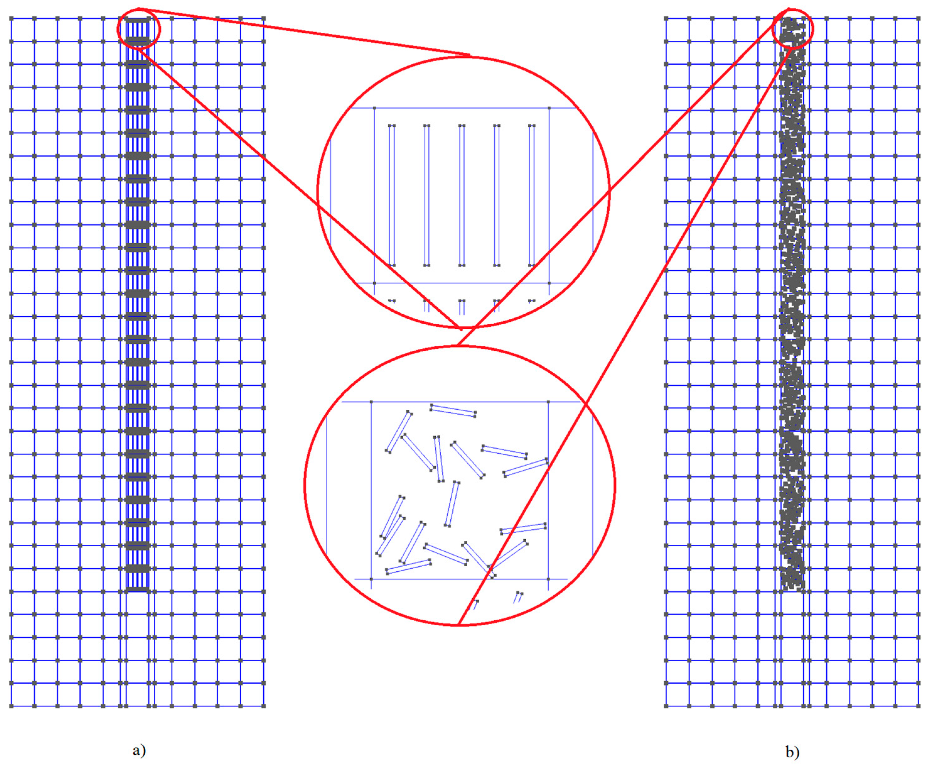
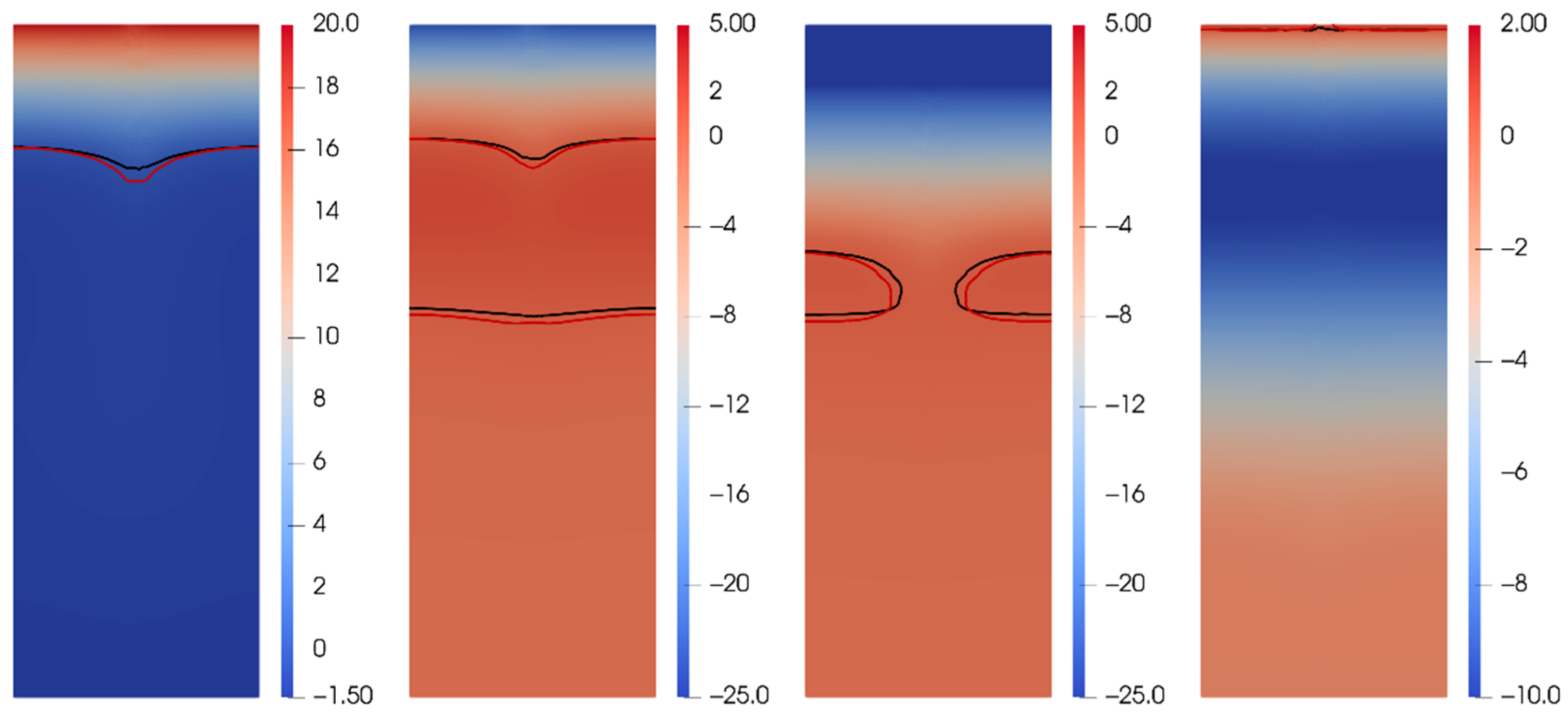
5. Numerical Results

In this section, the effect of fibers in a pile made of different materials on the temperature field of the soil is calculated. Thus, the melting effect of the pile is numerically simulated.

Conditions for the impact of piles on the temperature regime of the soil:

• Cement-sand mortar for filling the sinuses between the soil and the pile with a temperature of $+20{ }^{°}\mathrm{C}$;
• Piles with a cross section of 40 × 40 cm, pile deepening is 10 m from the ground surface.

The computational domain consists of several soil layers; it has one composite pile (Figure 2).

There are 4 cases which were considered:

• Fibers from basalt arranged in a structured manner;
• Fibers made of steel arranged in a structured manner;
• Fibers from basalt located randomly;
• Fibers made of randomly located steel.

Soil temperature is $1.5$ °C. Thermal-physical characteristics are taken from SP 25.13330.2012 and presented in

Table 2. Thermal-physical characteristics of soils.

Elements	Volumetric Heat Capacity $\mathit{c}\mathit{\rho } \ast {10}^{-6}$ (J/m3/K)		Thermal Conductivity $\mathit{k}$ (W/m/K)		Phase Transition Heat $\mathit{L} \ast {10}^{-3}$ (J/m3)
	Thawed	Frozen	Thawed	Frozen
Clay loam	3.17	2.41	2.67	2.84	101,600
Sand	2.31	2.14	2.15	2.37	114,800
Sand	2.78	2.26	2.26	2.62	101,600
Concrete	2.22		1.86		-
Basalt fiber	1.4		0.033		-
Steel fiber	368.8		53		-

. Calculations were performed for 365 days with a time step $\tau =1$ day (24 h).

The temperature of the daylight surface of the structure base was set considering the amplitude of the air temperature fluctuations taken from the data of the Yakutsk meteorological station. Figure 3 demonstrates the changes in the air temperature. It shows the distribution of the air temperature during one year.

Here are the results of numerical calculations. Figure 4 and Figure 5 show the soil temperature distributions for different points in time. These results were obtained by the GMsFEM method for eight basis functions.

For numerical comparison of the fine-scale and multiscale solutions, relative $L_2$ and energy errors are used.

$${\parallel e\parallel }_{L_2}=\sqrt{\frac{{{\displaystyle \int }}_{\mathsf{\Omega }}{\left(T_h-T_{ms}\right)}^{2}dx}{{{\displaystyle \int }}_{\mathsf{\Omega }}{T}_h{}^{2}dx},}{\parallel e\parallel }_a=\sqrt{\frac{a_{\varphi }\left(T_h-T_{ms,}{T}_h-T_{ms}\right)}{a_{\varphi }\left(T_h,T_h\right)},}$$

where $T_h$ and $T_{ms}$ are the fine-scale and multiscale solutions.

Table 3. Relative $L_2$ and energy errors (%) for different number of multiscale basis functions (DOFf = 172,681). Case 1: structured basalt fibers.

M	DOF	${\mathbf{\parallel }\mathit{e}\mathbf{\parallel }}_{{\mathit{L}}_2}$	${\mathbf{\parallel }\mathit{e}\mathbf{\parallel }}_{\mathit{a}}$
t = 50 days
2	744	0.86	7.48
4	1488	0.38	6.04
8	2976	0.15	3.21
t = 200 days
2	744	0.79	8.28
4	1488	0.39	6.63
8	2976	0.12	3.32
t = 250 days
2	744	0.27	5.64
4	1488	0.17	4.93
8	2976	0.05	2.84
t = 365 days
2	744	0.58	12.55
4	1488	0.28	10.35
8	2976	0.11	4.91

and

Table 4. Relative $L_2$ and energy errors (%) for different number of multiscale basis functions (DOF_f = 172,681). Case 2: structured steel fibers.

M	DOF	${\mathbf{\parallel }\mathit{e}\mathbf{\parallel }}_{{\mathit{L}}_2}$	${\mathbf{\parallel }\mathit{e}\mathbf{\parallel }}_{\mathit{a}}$
t = 50 days
2	744	2.86	22.43
4	1488	0.92	9.97
8	2976	0.47	7.28
t = 200 days
2	744	2.89	20.76
4	1488	0.86	9.41
8	2976	0.40	6.64
t = 250 days
2	744	2.16	21.31
4	1488	0.45	7.04
8	2976	0.21	5.34
t = 365 days
2	744	2.95	23.65
4	1488	0.42	13.82
8	2976	0.20	8.77

show the relative errors of $L_2$ and energies for different number of multiscale basis functions and corresponding degrees of freedom (DOF). Degrees of freedom for fine scale mesh is denoted as DOF_f. Here are the uncertainties for fibers arranged in structured order. When using basalt fibers, you can limit yourself to using 2 multiscale basis functions, and when using steel fibers, you need to use at least 4 multiscale basis functions.

Table 5. Relative $L_2$ and energy errors (%) for different number of multiscale basis functions (DOF_f = 207,599). Case 3: random distribution of basalt fibers.

M	DOF	${\mathbf{\parallel }\mathit{e}\mathbf{\parallel }}_{{\mathit{L}}_2}$	${\mathbf{\parallel }\mathit{e}\mathbf{\parallel }}_{\mathit{a}}$
t = 50 days
2	744	1.56	39.13
4	1488	0.57	12.36
8	2976	0.30	10.05
t = 200 days
2	744	1.66	39.74
4	1488	0.59	12.71
8	2976	0.31	10.27
t = 250 days
2	744	1.06	37.96
4	1488	0.32	10.65
8	2976	0.17	8.79
t = 365 days
2	744	1.07	42.13
4	1488	0.35	16.69
8	2976	0.17	12.96

and

Table 6. Relative $L_2$ and energy errors (%) for different number of multiscale basis functions (DOF_f = 207,599). Case 4: random distribution of steel fibers.

M	DOF	${\mathbf{\parallel }\mathit{e}\mathbf{\parallel }}_{{\mathit{L}}_2}$	${\mathbf{\parallel }\mathit{e}\mathbf{\parallel }}_{\mathit{a}}$
t = 50 days
2	744	2.40	14.64
4	1488	0.81	9.62
8	2976	0.37	6.13
t = 200 days
2	744	2.38	14.28
4	1488	0.80	9.49
8	2976	0.35	5.89
t = 250 days
2	744	1.30	11.41
4	1488	0.48	8.40
8	2976	0.18	4.78
t = 365 days
2	744	1.09	18.42
4	1488	0.49	13.36
8	2976	0.18	7.94

show the relative errors of $L_2$ and energies for different number of multiscale basis functions for case, when fibers are located randomly. It can be seen that using four multiscale basis functions leads to good accuracy.

A comparison was also made for different fiber arrangements (Figure 6 and Figure 7). As the figures show, random arrangement of the fibers is better. However, this may be due to the fact that they are located horizontally.

6. Discussion

For the solution of the Stefan problem related to the soil thawing effect of composite piles, GMsFEM was used. According to results showing the accuracy of the method, the usage of four basis functions leads to the results with error in L₂ norm lower than 1%. The errors in energy norms are also very respectable. Thus, usage of GMsFEM for such problems is recommended.

Results show that the process of total freezing of piles with steel fiber inclusion in winter runs faster. Analysis shows that the length between isoclines of phase change is about 47 cm for structured and 37 for random distribution of fibers. Freezing of pile with steel fibers comes on the 239th day, and a pile with basalt inclusion freezes on the 250th day in the structured case. For random distribution, similar days are 245th and 252nd. Therefore, there are 11 and 7 days’ delay between freezing of piles with steel and fiber inclusions, depending on the distribution.

7. Conclusions

In this work, the effect of a composite pile on the temperature field of the surrounding frozen soil using GMsFEM is considered. Results of calculations using GMsFEM show good accuracy. It can be said that when using materials with higher thermal conductivity, the thermal regime restores faster. In the future, we plan to consider the problems in the 3D statement and work with the piles with more complex compositions.

References

- Vasiliev, V.I.; Sidnyaev, N.I.; Fedotov, A.A.; Ilyina, Y.u.S.; Vasilieva, M.V.; Stepanov, S.P. Modeling the Distribution of Non-Stationary Temperature Fields in the Permafrost Zone in the Design of Geotechnical Structures; Kurs: Moscow, Russia, 2017. [Google Scholar]
- Nagy, B.; Nehme, S.G.; Szagri, D. Thermal Properties and Modeling of Fiber Reinforced Concretes. Energy Procedia 2015, 78, 2742–2747. [Google Scholar] [CrossRef] [Green Version]
- Zhussupbekov, A.; Shin, E.C.; Shakhmov, Z.; Tleulenova, G. Experimental study of model pile foundations in seasonally freezing soil ground. Int. J. GEOMATE 2018, 15, 85–90. [Google Scholar] [CrossRef]
- Montayeva, A.; Zhussupbekov, A.; Kaliakin, V.N.; Montayev, S. IOP Conference Series: Earth and Environmental Science; Analysis on Technological Features of Pile Foundations Construction in Frozen and Seasonal Thawing Soils, No. 1; IOP Publishing: Bristol, UK, 2021; p. 012006. [Google Scholar]
- Jiang, C.; Fan, K.; Wu, F.; Chen, D. Experimental study on the mechanical properties and microstructure of chopped basalt fibre reinforced concrete. Mater. Des. 2014, 58, 187–193. [Google Scholar] [CrossRef]
- High, C.; Seliem, H.M.; El-Safty, A.; Rizkalla, S.H. Use of basalt fibers for concrete structures. Constr. Build. Mater. 2015, 96, 37–46. [Google Scholar] [CrossRef]
- Smarzewski, P. Study of Bond Strength of Steel Bars in Basalt Fibre Reinforced High Performance Concrete. Crystals 2020, 10, 436. [Google Scholar] [CrossRef]
- Fiore, V.; Scalici, T.; Di Bella, G.; Valenza, A. A review on basalt fibre and its composites. Compos. Part. B Eng. 2015, 74, 74–94. [Google Scholar] [CrossRef]
- Branston, J.; Das, S.; Kenno, S.Y.; Taylor, C. Mechanical behaviour of basalt fibre reinforced concrete. Constr. Build. Mater. 2016, 124, 878–886. [Google Scholar] [CrossRef]
- Caggiano, A.; Folino, P.; Lima, C.; Martinelli, E.; Pepe, M. On the mechanical response of Hybrid Fiber Reinforced Concrete with Recycled and Industrial Steel Fibers. Constr. Build. Mater. 2017, 147, 286–295. [Google Scholar] [CrossRef]
- Leone, M.; Centonze, G.; Colonna, D.; Micelli, F.; Aiello, M.A. Experimental Study on Bond Behavior in Fiber-Reinforced Concrete with Low Content of Recycled Steel Fiber. J. Mater. Civ. Eng. 2016, 28, 04016068. [Google Scholar] [CrossRef]
- Mastali, M.; Dalvand, A. Use of silica fume and recycled steel fibers in self-compacting concrete (SCC). Constr. Build. Mater. 2016, 125, 196–209. [Google Scholar] [CrossRef]
- Sengul, O. Mechanical behavior of concretes containing waste steel fibers recovered from scrap tires. Constr. Build. Mater. 2016, 122, 649–658. [Google Scholar] [CrossRef]
- Caggiano, A.; Xargay, H.; Folino, P.; Martinelli, E. Experimental and numerical characterization of the bond behavior of steel fibers recovered from waste tires embedded in cementitious matrices. Cem. Concr. Compos. 2015, 62, 146–155. [Google Scholar] [CrossRef]
- Aiello, M.A.; Leuzzi, F.; Centonze, G.; Maffezzoli, A. Use of steel fibres recovered from waste tyres as reinforcement in concrete: Pull-out behaviour, compressive and flexural strength. Waste Manag. 2009, 29, 1960–1970. [Google Scholar] [CrossRef]
- Samarskii, A.A.; Vabishchevich, P.N. Computational Heat Transfer; Wiley: Chichester, UK, 1995. [Google Scholar]
- Bernauer, D.I.M. Motion Planning for the Two-Phase Stefan Problem in Level Set Formulation. Ph.D. Thesis, Chemnitz University of Technology, Chemnitz, Germany, 2010. Available online: https://core.ac.uk/download/pdf/153228887.pdf (accessed on 25 June 2021).
- Vasil’ev, V.; Vasilyeva, M. An Accurate Approximation of the Two-Phase Stefan Problem with Coefficient Smoothing. Mathematics 2020, 8, 1924. [Google Scholar] [CrossRef]
- Vasilyeva, M.; Stepanov, S.; Spiridonov, D.; Vasil’Ev, V. Multiscale Finite Element Method for heat transfer problem during artificial ground freezing. J. Comput. Appl. Math. 2020, 371, 112605. [Google Scholar] [CrossRef]
- Stepanov, S.; Vasilyeva, M.; Vasil’Ev, V.I. Generalized multiscale discontinuous Galerkin method for solving the heat problem with phase change. J. Comput. Appl. Math. 2018, 340, 645–652. [Google Scholar] [CrossRef]
- Efendiev, Y.; Galvis, J.; Hou, T.Y. Generalized multiscale finite element methods (GMsFEM). J. Comput. Phys. 2013, 251, 116–135. [Google Scholar] [CrossRef] [Green Version]
- Efendiev, Y.; Hou, T.Y. Multiscale Finite Element Methods: Theory and Applications; Springer Science & Business Media: Berlin, Germany, 2009; Volume 4. [Google Scholar]
- Efendiev, Y.; Ginting, V.; Hou, T.Y. Multiscale Finite Element Methods for Nonlinear Problems and Their Applications. Commun. Math. Sci. 2004, 2, 553–589. [Google Scholar] [CrossRef] [Green Version]
- Xing, Y.F.; Yang, Y.; Wang, X.M. A multiscale eigenelement method and its application to periodical composite structures. Compos. Struct. 2010, 92, 2265–2275. [Google Scholar] [CrossRef]
- Hou, T.Y.; Wu, X.H. A multiscale finite element method for elliptic problems in composite materials and porous media. J. Comput. Phys. 1997, 134, 169–189. [Google Scholar] [CrossRef] [Green Version]
- Alghamdi, A.; Alharthi, H.; Alamoudi, A.; Alharthi, A.; Kensara, A.; Taylor, S. Effect of Needling Parameters and Manufacturing Porosities on the Effective Thermal Conductivity of a 3D Carbon–Carbon Composite. Materials 2019, 12, 3750. [Google Scholar] [CrossRef] [PubMed] [Green Version]
- Tomkova, B.; Sejnoha, M.; Novak, J.; Zeman, J. Evaluation of effective thermal conductivities of porous textile composites. Int. J. Multiscale Comput. Eng. 2008, 6, 153–167. [Google Scholar] [CrossRef]
- Ai, S.; Fu, H.; He, R.; Pei, Y. Multi-scale modeling of thermal expansion coefficients of C/C composites at high temperature. Mater. Des. 2015, 82, 181–188. [Google Scholar] [CrossRef]
- Zhao, Y.; Song, L.; Li, J.; Jiao, Y. Multi-scale finite element analyses of thermal conductivities of three dimensional woven composites. Appl. Compos. Mater. 2017, 24, 1525–1542. [Google Scholar] [CrossRef]