Article

Assessment of Analytical Orientation Prediction Models for Suspensions Containing Fibers and Spheres

1
Fraunhofer IWM, Wöhlerstraße 11, 79108 Freiburg, Germany
2
Mechanical Process Engineering and Solids Processing (MVTA), TU Berlin, Ernst-Reuter-Platz 1, 10587 Berlin, Germany
*
Author to whom correspondence should be addressed.
J. Compos. Sci. 2021, 5(4), 107; https://doi.org/10.3390/jcs5040107
Submission received: 23 March 2021 / Revised: 8 April 2021 / Accepted: 12 April 2021 / Published: 13 April 2021
(This article belongs to the Special Issue Characterization and Modelling of Composites, Volume II)

Abstract

:
Analytical orientation models like the Folgar Tucker (FT) model are widely applied to predict the orientation of suspended non-spherical particles. The accuracy of these models depends on empirical model parameters. In this work, we assess how well analytical orientation models can predict the orientation of suspensions not only consisting of fibers but also of an additional second particle type in the shape of disks, which are varied in size and filling fraction. We mainly focus on the FT model, and we also compare its accuracy to more complex models like Reduced-Strain Closure model (RSC), Moldflow Rotational Diffusion model (MRD), and Anisotropic Rotary Diffusion model (ARD). In our work, we address the following questions. First, can the FT model predict the orientation of suspensions despite the additional particle phase affecting the rotation of the fibers? Second, is it possible to formulate an expression for the sole Folgar Tucker model parameter that is based on the suspension composition? Third, is there an advantage to choose more complex orientation prediction models that require the adjustment of additional model parameters?

1. Introduction

1.1. Motivation

Mechanical properties of fiber-reinforced engineering materials often depend on their local orientation of fibers [1,2]. For example, specimens are reported to be stronger in the direction of fiber alignment [3], or the alignment of the fibers influences the thermal conductivity in sheet layers [4]. Consequently, there is a desire to predict the orientation for a specific process to optimize a part with respect to a specific mechanical property. The problem set up for investigation is illustrated in Figure 1, which shows an exemplary extrusion process in which a paste filled with fibers and spheres is extruded through a nozzle. The final orientation of the fibers in the extruded filament is complex to predict as it arises from an interplay of experienced hydrodynamic forces and interactions between the particles during the printing process.
Several strategies exist to predict the orientation of fibers. One obvious strategy is to perform experiments and measure the orientation of the fibers [5]. This approach is, however, tedious and time-consuming, and therefore numerical tools may facilitate collating information. Among the numerical tools, there exist two fundamental approaches working on different scales. On the one hand, Direct Numerical Simulations(DNS) can be applied on a particle scale, which means that the particles and the flow around them is fully resolved. Methods on this scale mainly differ in the choice whether the momentum of the particle phase is mapped back onto the fluid phase [6,7] (so called two-way coupling(TWC)), or not [2,8] (so called one-way coupling(OWC)), but they all provide the advantage that the orientation of particles can be measured. On this scale, it is also possible to include complex interactions such as surface chemistry [9], magnetism [10], or drying [11]. The disadvantage of these methods is that they are computationally too expensive to simulate the whole specimen being filled with particles with todays computational resources in reasonable time [12]. Therefore, on the other hand, a more pragmatic approach does not resolve the particles any more, and for this reason, it can be applied on the scale of the specimen [13,14]. This approach combines a fluid solver with an analytical prediction model, where the fluid solver predicts the velocity profile and provides this information to the analytical model that predicts the orientation. The quality of the orientation prediction thereby depends on the resolution of the fluid solver and the applicability of the prediction model for the given suspension and process conditions.

1.2. Measuring Fiber Orientation States by Orientation Tensors

We assign a unit orientation vector p to each fiber that coincides with its principle axis. The ensemble average of all orientation vectors provide a concise description of the local orientation state in terms of a second order orientation tensor A , with [15]
A = p p p ψ ( p ) d p ,
where ψ ( p ) is the orientation distribution function.

1.3. Orientation Prediction by Jeffery and Folgar Tucker

Multiple analytical prediction models exist, two famous ones are the models of Jeffery [16] and Folgar Tucker(FT) [17]. Jeffery’s model became famous for its correct orientation prediction within a suspension of arbitrarily shaped particles in all kinds of flow fields and the only limitation of the model is that the concentration must be dilute (i.e., filling fraction ϕ < ( 1 / a r ) 2 , with aspect ratio a r ) [17] to ensure insignificant particle interactions. The model of Jeffery is given by
d A d t = W · A A · W + λ D · A + A · D 2 D : A
with a material derivate d / d t , a vorticity tensor W = 1 2 v v T , a rate of strain tensor D = 1 2 v + v T , a velocity gradient v , a form factor λ = ( a r 2 1 ) / ( a r 2 + 1 ) to consider the shape of the fibers, a unit tensor 1 ̲ , and a fourth order orientation tensor A . The fourth order tensor A is an unknown quantity in Equation (2) that is usually approximated as a function of the second order tensor by means of a closure approximation; in this work, the commonly applied hybrid closure approximation is used [18]. In this approximation, the elements A i j k l of A are derived based on a combination of the linear [19] and the quadratic closure approximation [20,21] by [15,18] A i j k l = ( 1 f ) A ^ i j k l + f A ˜ i j k l , where the linear closure approximation is given by A ^ i j k l = c 1 ( δ i j δ k l + δ i k δ j l + δ i l δ j k ) + c 2 ( a i j δ k l + a i k δ j l + a i l δ j k + a k l δ i j + a j l δ i k + a j k δ i l ) with c 1 = 1 / 24 , c 2 = 1 / 6 in two-dimensional(2D) and c 1 = 1 / 35 , c 2 = 1 / 7 in three-dimensional(3D) formulations, δ i j as the Kronecker operator and a i j being the element of the second order tensor A , the quadratic closure approximation is given by A ˜ i j k l = a i j a k l , and a blending factor f, which in 2D is given by f = 2 a i j a j i 1 and in 3D by f = 3 / 2 a i j a j i 1 / 2 . Additionally, we also apply the Invariant-based optimal fitting(IBOF) of Du Chung et al. that is exactly applied as explained in reference [22] for the 3D case and in reference [23] for the 2D case.
An orientation model that can also be applied to dense suspensions (i.e., ϕ > ( 1 / a r ) 2 ) is the FT model that provides an extension to the Jeffery model to consider the particles’ interaction in dense suspensions. This extension introduces a phenomenological model parameter—the FT parameter C I —to quantify the particles’ interactions. The FT model belongs to the class of Isotropic Rotary Diffusion(IRD) models as the C I parameter equally affects the orientation prediction in all dimensions. The FT model in tensor notation is given by [18]
d A d t = W · A A · W + λ D · A + A · D 2 D : A + 2 C I γ ˙ 1 ̲ d A ,
with a scalar shear rate γ ˙ = 2 D : D . From all variables in Equation (3), the FT parameter C I is the only parameter free to choose and all other parameter either arise from flow conditions or from the shape of the particles or the underlying closure approximation.
Many authors have determined the FT parameter, as shown in Figure 2, and often the parameter is provided as a function of the product of filling fraction of fibers ϕ f and the aspect ratio of the fibers a r . Despite the importance of the FT parameter, there exist contradicting trends and ideas about the FT parameter that is reported to range over at least five orders of magnitude. For example, Bay [24] and Mezher et al. [25] assume that C I should decrease with ϕ f a r ; while Phan Thien et al. [26], Folgar and Tucker [17], Meyer et al. [7], and Fan et al. [27] report it to increase. A different dependency is published by Ranganathan and Advani [28], who suggest that when the model parameter is describing the particle–particle interactions, then it must depend on the local particle orientation and therefore change over time (decreasing from 0.6 to 0.05 in their work). They summarized their findings into an equation that does not depend on suspension parameter directly, but on a mean distance between the fibers and a fitting parameter that should, however, be independent of the suspension. The mean distance between the fibers cannot be mapped to ϕ f a r , and therefore the shaded area in Figure 2 is a free interpretation of their statement to only visualize the order of magnitude in which they reported their FT parameter. All in all, although explanations for the variation in trends exist [29], we find a strong deviation of reported parameters among most authors, which shows that the knowledge towards an optimal FT parameter has not yet fully converged.

1.4. Further Analytical Orientation Prediction Models

Further prediction models have been introduced, most of which can be divided into two classes. One class [30,31] slows down the orientation rate to handle the phenomena that the Jeffery and FT models reach the steady-state within less strain than observed in corresponding experiments. These models have little influence on the predicted steady-state. A second class, Anisotropic Rotary Diffusion(ARD) [32], allows one to control the steady state within each dimension individually. Models that combine elements from both classes exist to fine-tune both the steady-state itself and the speed with which this steady state is reached. A detailed presentation of all existing models is beyond the scope of this manuscript, and we refer the interested reader to references [33,34] for a detailed comparison of all models or anisotropic models in particular. Table 1 shows an incomplete list of some commonly used prediction models from both classes. While each of the models is motivated by and designed for a different physical phenomena, we reduce them to their number of model parameter in this work. What all models again have in common is the non-existence of a concrete equation to compute the model parameters; instead, they have to be fitted against experimental data. Therefore, models that are more powerful might be available but the problem that we have been confronted with in the case of the FT model—not knowing the model parameter—still persists.
In this work, we mainly address two research questions. First, to what degree can the FT model predict the orientation within various suspensions although the model provides only one fitting parameter? Second, should more powerful orientation prediction models be preferred? The novelty of this work is that the suspension under consideration consists of two different particle shapes, i.e., round particles and elongated particles that we relate to as disks and fibers, respectively. We varied the suspension parameter in terms of (a) the filling fraction of disks and fibers, (b) the size of the disks and (c) the aspect ratio of the fibers. The data on which this work is based on are openly accessible from reference [37].
This work is structured as follows. Section 2 briefly describes the fundamentals behind the numerical simulations of the suspension simulations that are used as a basis to fit the FT parameter. Section 3 shows the results of the individually fitted FT parameters, and it compares the accuracy of various prediction models to predict our simulated orientation. Section 4 discusses the results with the help of snapshots from selected simulations. Section 5 concludes this work.

2. Method

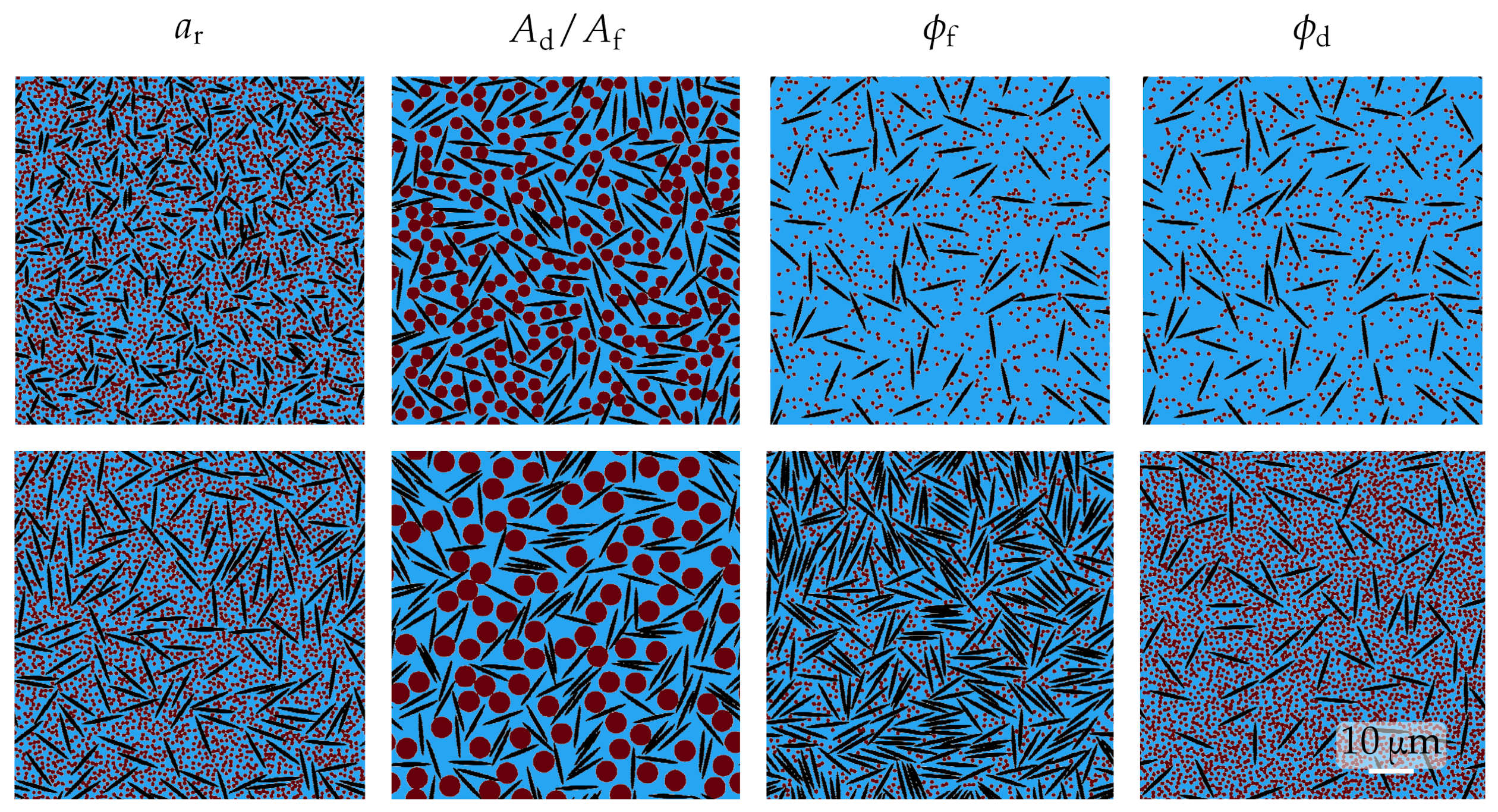
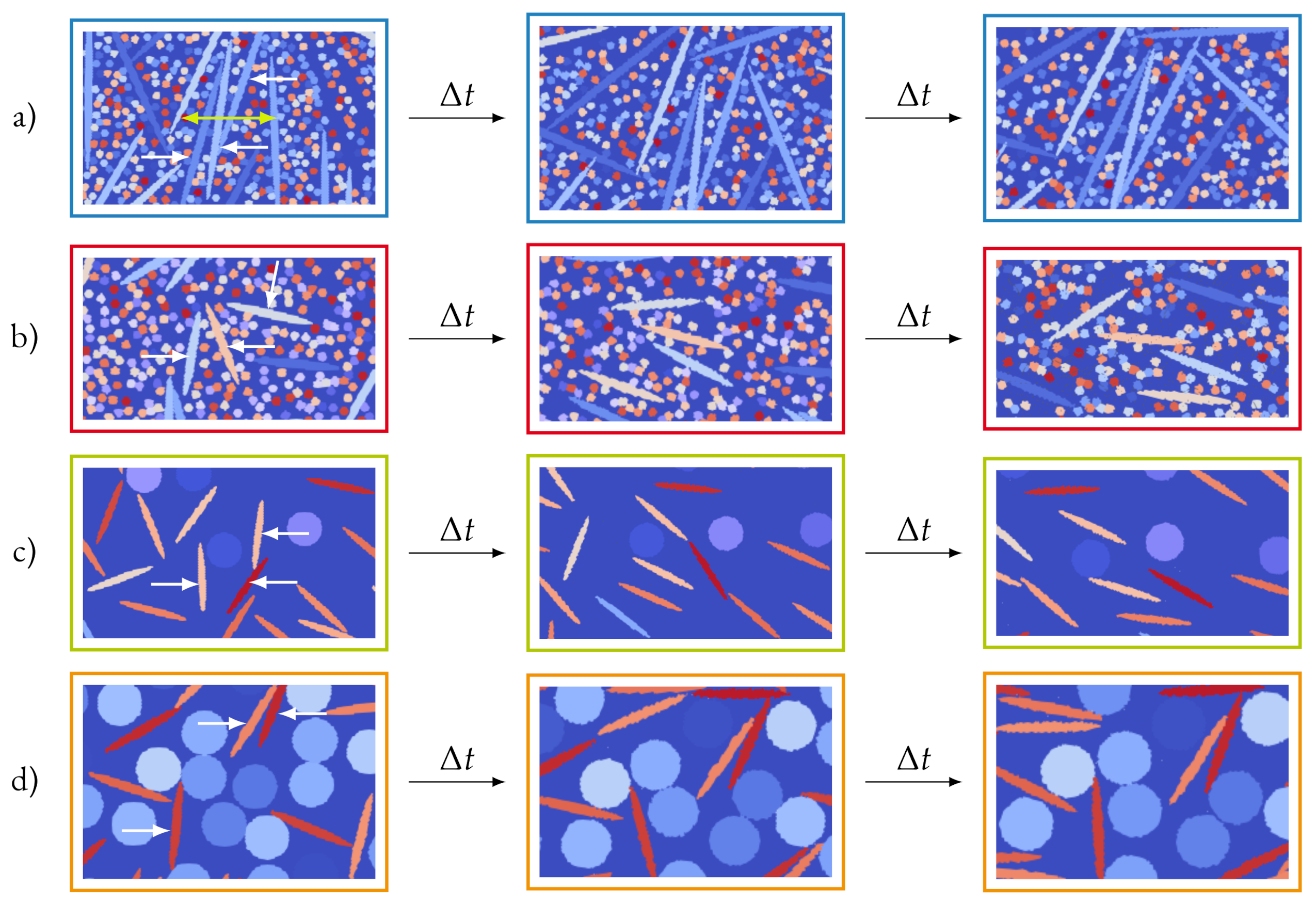
2.1. Suspension Simulations

Non-Brownian suspension simulations are applied to provide the orientation data against which we fitted the FT parameter. The algorithm and setup for the suspension simulations are precisely described and validated in reference [38]. A validation to an experiment showing that the model is able to predict the orientation accurately is presented in reference [39]. For the sake of brevity, we only summarize the fundamentals and refer the reader to the references for a deeper understanding of the scheme. We perform 2D simulations with Smoothed Particle Hydrodynamics (SPH) that is used to discretize the particle phase and the surrounding fluid phase with a direct coupling between both phases, which means that the local orientation of the particles has a direct influence on the local fluid phase and vice versa. The particles interact with each other by repulsion and friction forces, and the fluid is described by a Newtonian rheology model.
Some examples of the numerical setup are shown in Figure 3, in which we show the fibers in black, the disks in red and the surrounding fluid phase in blue. Figure 3 shows examples of the variation of four parameters of the present study: aspect ratio a r of the fibers, the disk size and thereby the ratio of disk to fiber size A d / A f , and the filling fraction of fibers ϕ f and disks ϕ d .
Three types of deformation are applied within an Representative Volume Element(RVE) as illustrated in Figure 4 in terms of shear (subfigure a), elongation (subfigure b) or a combination of both (subfigure c). The product of γ ˙ t is used to quantify the amount of deformation.

2.2. Computation of FT Parameters

An FT parameter is retrieved by the following procedure. First, the orientation tensor is computed for a simulation. Second, we predict an orientation applying Equation (3) with exactly the same velocity gradient as used in the simulation and an initial orientation tensor as present in the simulation at t = 0 s . The FT parameter was used as a free fitting parameter to minimize the deviation between numerical simulation and FT prediction by a least mean square error method. An exemplary result is shown in Figure 5. Thereby, the FT parameter is chosen such that the whole transient evolution of the whole orientation tensor is most accurately described. The result of this procedure is therefore one FT parameter for each simulation.

3. Results

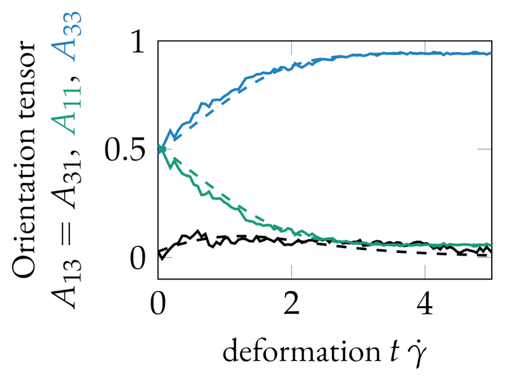
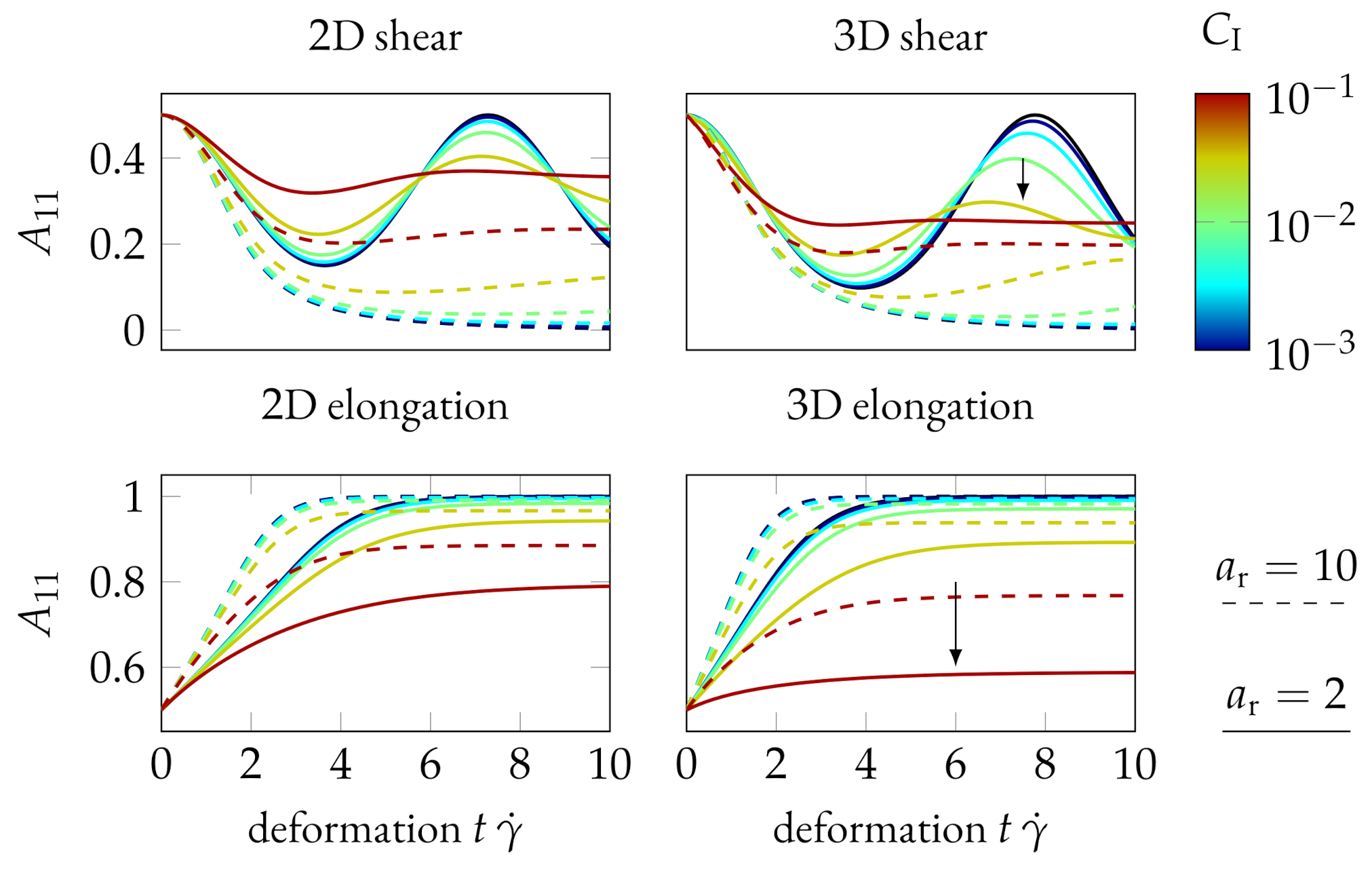
3.1. Influence of the FT Model Formulation

While the governing equation of the FT model is precisely described, its implementation allows a certain degree of freedom when it comes to the closure approximation (see Section 1.3). In this section, we want to study the effect of the FT model formulation on the resulting FT parameter. In particular, we want to compare the quadratic, hybrid. and IBOF closure approximation as well as the influence of whether the 2D or 3D formulation is applied. The simulations are performed in 2D, and therefore the default formulation applied in this work is the 2D formulation of the FT model in combination with the hybrid closure approximation if not stated differently.
We study the influence of the 2D and 3D formulation of the FT model on the orientation prediction. Figure 6 shows the A 11 component of the orientation tensor of the 2D (left) and 3D (right) formulation of the FT model for the case of shear (top) and elongation (bottom), for five different FT parameters (color coded according to colorbar), and two different aspect ratios (solid and dashed line). A comparison between the left and right subfigures shows that there is a clear difference in orientation prediction between the 2D and 3D formulation that becomes more obvious with increasing C I (see arrows). The black line in Figure 6 denotes the solution according to the Jeffery model (Equation (2)). We find the FT model with C I 10 3 to be barely distinguishable from the Jeffery model in the 3D shear case and indistinguishable in all other cases. It should be noted that we performed our simulation in 2D, and the conclusion being drawn in this work might be different based on 3D simulations.
Up to this point, we have studied the orientation prediction of the FT model purely based on the model formulation. Now we move on to the results of the particle simulation for the remaining part of this results section. From here onward, we relate to the FT parameters that have been fitted as explained in Section 2.2.
We study the influence of the FT model formulation (dimensionality and closure approximation) on the FT parameter. As we gave learned, the dimensionality and the closure approximation affect the orientation prediction, and the fitting routine towards the numerical data yields different parameters for each formulation. A histogram of FT parameters among all simulations for each FT model formulation is shown in Figure 7, in which each column corresponds to one specific closure approximation. The top row shows the histogram of parameters contrasting the effect the of dimensionality for a specific closure, and the bottom row shows a scatter plot in which each point denotes one pair of C I from the 2D and 3D formulation to show the correlation between both.
We see that the 3D formulation in general yields significantly smaller FT parameters than the 2D formulation. We also find the IBOF closure to yield smaller C I than the hybrid closure, whose C I parameters are again smaller than for the quadratic closure. There is a correlation (Pearson correlation test) of 0.93 and 0.91 for the quadratic and hybrid closure, and only of 0.6 for the IBOF closure. The reason for this difference in correlation among the closures in discussed in Section 4.1.

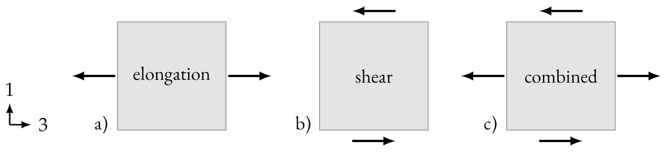
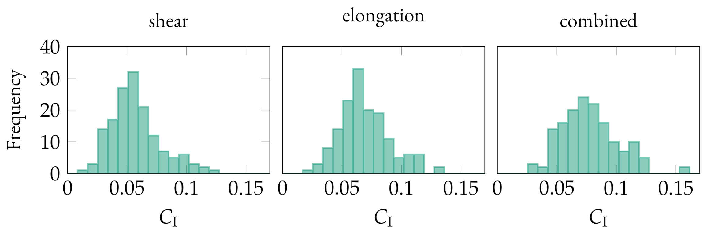
3.2. Influence of the Flow Type

The FT model predicts the orientation for a flow of all kinds of velocity gradients. In our simulations, we applied three different kinds of velocity gradient (shear, elongation, or a combination of both), and in this section, we study to what degree the FT parameters vary with flow type. Figure 8 shows a histogram of FT parameters originating from all suspensions from one specific flow type. We find all flow types to yield similar distribution of FT parameters with respect to peak position ( C I = 0.06 ) as well as minimum and maximum FT parameters.

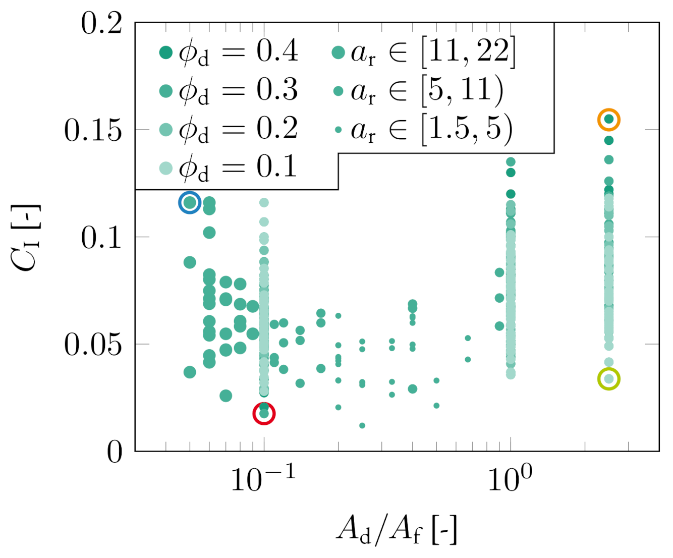
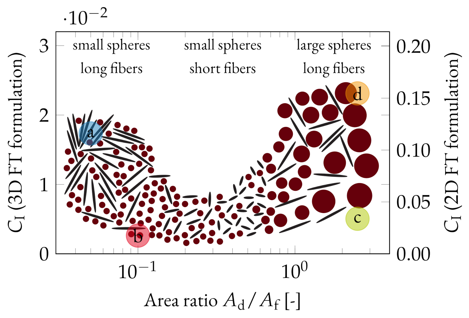
3.3. Influence of Disk Size

The main purpose of this paper is to assess to what degree the FT model can predict the orientation in suspensions including a secondary disk phase. We performed simulations with varying fiber aspect ratio, disk size, and filling fraction of fibers and disks, and the resulting FT parameters are shown in Figure 9. The abscissa denote the area ratio A d / A f of one single disk to one single fiber, while all disks and all fibers have the same size in one suspension. As such, the abscissa describes the transition from very small to large disks in relation to the fibers. Every simulation yields one single FT parameter that is represented by a point where the size and the color of the point describes the suspension composition: the size of the point represents the aspect ratio of the fibers where small points represent small and large points large aspect ratios, and the color of the point shows the underlying filling fraction of disks in the suspension where a dark green relates to a high filling fraction of disks.
The point cloud originates from three classes: first, the region with A d / A f 0.2 describes suspensions with long fibers and disks small in size compared to the fibers; second, for 0.2 < A d / A f < 1.0 , the suspensions are composed of short fibers and disks that are still smaller than the fibers; third, for 0.8 A d / A f , we have suspensions with long fibers and disks of equal or larger size. The FT parameters are generally widely distributed among all suspensions and classes. The highest FT parameters are generally found to be highest in the third region (large disks), followed by the first region (long fibers), and the smallest maximum FT parameter is found in the second region (small fibers). The majority of points in Figure 9 originate from a suspension with filling fraction of fibers ϕ f = 0.2 and disks ϕ d = 0.3 , and both filling fractions have only been varied for A d / A f { 0.1 , 1 , 2.5 } ; hence, lighter green colors appear only at these positions. For A d / A f = 0.1 , the highest FT parameter is found among the suspensions with the highest amount of long fibers (please note that the coloring of the point describes the filling fraction of disks and not of fibers, and the filling fraction of fibers cannot be extracted from the figure) and is lowest for the suspension with a low amount of long fibers. For A d / A f = 1 , and A d / A f = 2.5 , contrariwise, the FT parameter is highest for those suspensions with many large disks and lowest for those suspensions with few large disks. Four FT parameters in Figure 9 are marked by a colored ring, and the underlying simulation yielding this parameter is discussed in Section 4.3.

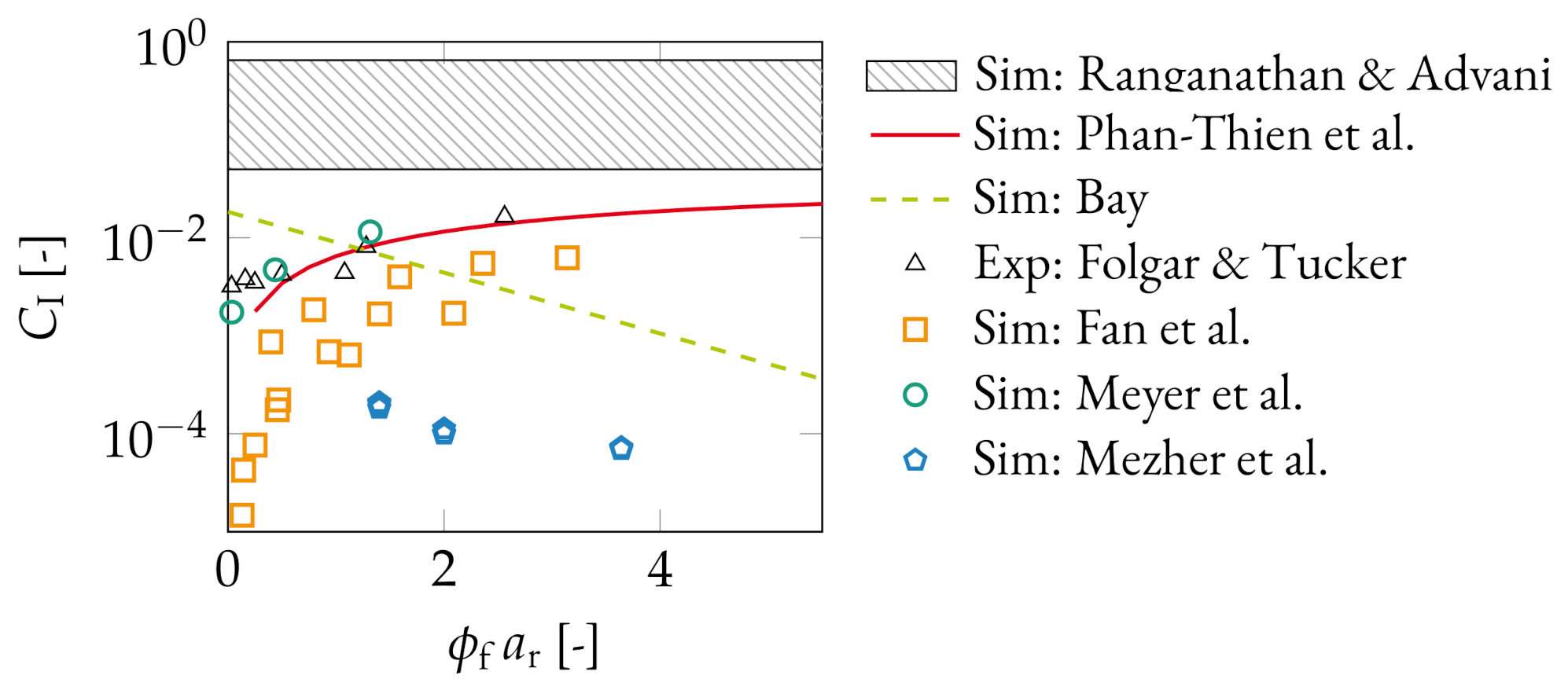
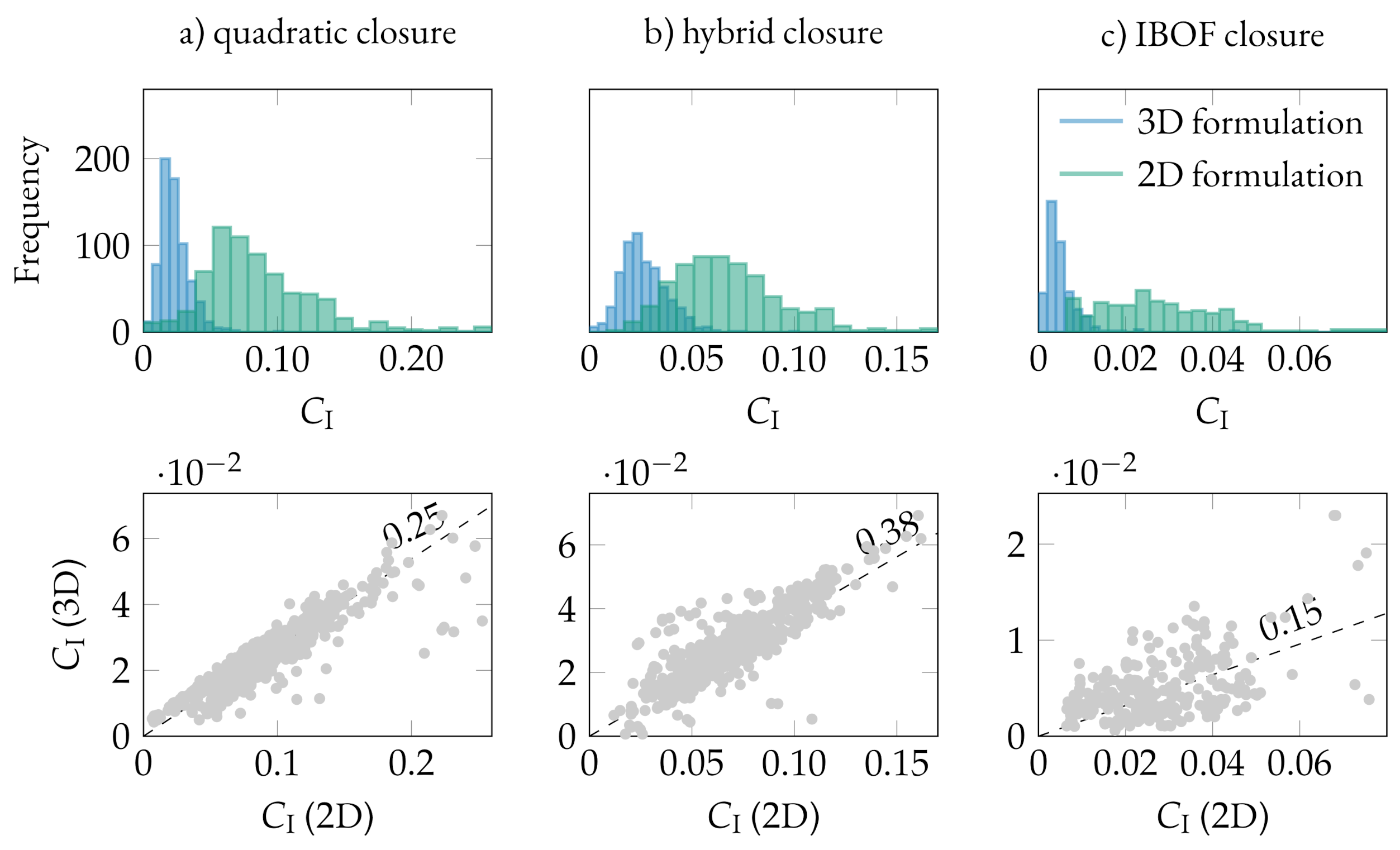
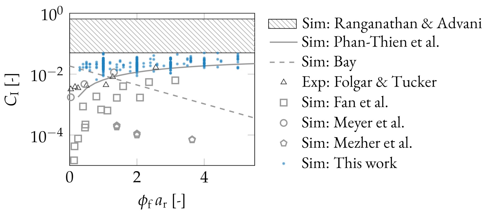
3.4. Comparison of Existing Data

We compare our FT parameters in Figure 10 with those from the literature, which are shown in Figure 2. Here, we exceptionally use the parameters obtained from the 3D formulation of the FT model, as this is the formulation applied by all authors. The data being shown in Figure 2 include only those suspension simulations with no or only small disks. The data themselves are found in the same order of magnitude as those published by Phan-Thien et al., Folgar and Tucker, and Bay. A detailed discussion of the comparison with other authors is provided in Section 4.4.

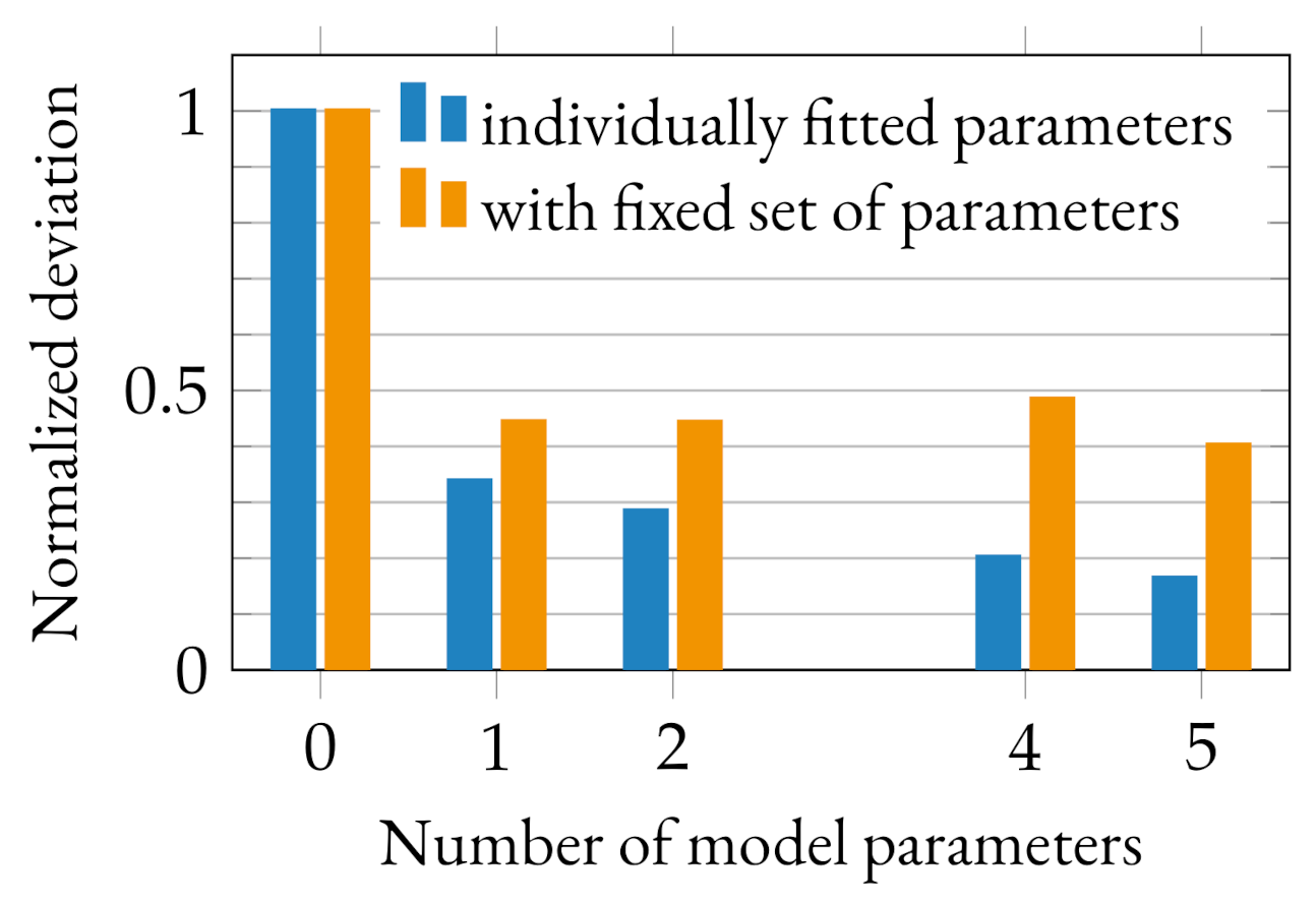
3.5. Accuracy of FT Model in Contrast to Other Analytical Orientation Prediction Models

Various analytical prediction models exist and four of them are compared to the FT model in this section with regard to their accuracy to predict the orientation provided by the simulation. The first model, the Jeffery model, is a special case because it does not have any fitting parameters, nor is it designed to be applied for dense suspensions. The second model is the FT model with only one fitting parameter. The third model, the RSC model, is similar to the FT model, but it provides an additional parameter to fine-tune the speed with which the steady-state orientation is reached. The fourth model, the Moldflow Rotational Diffusion(MRD) model, has a structure similar to the FT model, but it involves three additional parameters to fine-tune the orientation alignment rate with the current orientation tensor. The fifth model, the ARD model, applies an additional anisotropic rotary tensor, which is given as a function of five parameters. We chose these models as there is a parameter set for which all models restore the FT model, or Jeffery model, respectively, and should be able to outperform this model. At this point, each model is characterized only by the number of model parameters.
In Figure 11, we assess the accuracy of all models to predict the orientation of suspensions, which means we compare the deviation between the analytical prediction and the simulation. Two cases are distinguished: the blue bars describe the case in which the analytical model has been fitted to every of our simulations individually with all fitting parameters being available, and the orange bars describe the case in which we have applied a fixed set of model parameters to predict the orientation among all suspensions independent of their composition. The parameters chosen for the second case are thereby extracted from the parameters obtained by the fitting routine. We always chose the parameter which in a histogram describes the peak position, as this value is expected to best describe all suspensions (for example, for FT, we used C I = 0.06 as described in Section 3.2). The orange bars represent the case in which a perfect model parameter is unknown and has been retrieved by a fitting routine towards available data. Studying only the blue bars, we see that the total deviation reduces with increasing number of model parameters, and the largest reduction in deviation is obtained from moving from the Jeffery model to the FT model. When we focus on the orange bars with fixed parameters, we see that the deviation among all models with fitting parameters is similar.

4. Discussion

The FT model is a widely applied analytical orientation prediction model. The equation itself is designed in such a way that all surrounding process conditions, i.e., the local velocity field, are fully considered, and what remains is only the FT parameter that, in theory, should only depend on the suspension parameters. From a mathematical point of view, the FT parameter regulates a dissipation term, which means that increasing the FT parameter either lowers the final steady-state orientation in elongation flow or it lowers the magnitude of the oscillation under shear flow. The value of the FT parameter itself has no direct meaning, but an increase in the FT parameter can be interpreted as showing that the particles are more hindered in their rotation. This link should be kept in mind for the remainder of this discussion, as we will use this analogy to explain why the FT parameter increases or decreases in some simulations.

4.1. Formulation

While the FT model is precisely formulated, its implementation adds a degree of freedom towards the choice of the closure approximation. In this work, we started with the influence of the choice of this closure approximation and, additionally, if the 2D or 3D formulation of the model is applied. We found that both the formulation and closure approximation significantly affect the FT parameter. For the same closure approximation, the 3D model yields smaller FT parameters than the 2D. Basically, this means that the same FT parameter has a stronger influence on the orientation prediction in 3D than in 2D. The reason for this behavior is unintuitive but understandable when we have a closer look at the term 2 C I γ ˙ 1 ̲ d A that has been added to the Jeffery model. Let us consider an orientation tensor that describes the steady state in which the A 11 entry of the orientation tensor is approaching unity. In this example, the term 1 d A (looking only at A 11 ) yields 1 3 × 1 = 2 or 1 2 × 1 = 1 in 3D, or 2D, respectively. This means that the material derivative is larger in 3D than in 2D, and, therefore, the corresponding FT parameter must be chosen smaller in 3D than in 2D to give the same orientation prediction. Hence, the FT parameter has a stronger influence on the orientation prediction in 3D than in 2D, which simultaneously means that the 2D model needs significantly larger values to adjust the orientation curves. Even more interesting than the influence of the 2D vs. 3D formalism is the influence of the closure approximation. We find FT parameters with the quadratic and hybrid closure to be significantly larger than when applying the IBOF closure. This behavior that the FT parameters with the IBOF closure are significantly smaller is unsurprising if we follow the strategy of Du Cheng et al. [22] to formulate this closure approximation. They provide a set of 63 fitting parameters, all of which have been fitted to numerical data that have been created assuming C I = 0 . As such, the closure is designed in such a way that the hydrodynamic part (i.e., the Jeffery part without the FT extension) is already capable of predicting a reasonable orientation within the suspension. Therefore, the magnitude with which the FT extension has to correct the prediction by the hydrodynamic part is obviously smaller and this correlates to a small FT parameter. There exist other closure methods (e.g., NAT [23], OWR [40], OWR3 [41]) that have not been tested in this but in other works (e.g., [34]) coming to the same conclusion that the choice of closure has a significant impact on the orientation prediction. We also find a high correlation between the C I values for the 2D and 3D formulation for the hybrid and quadratic closure, while the correlation was found lower for the IBOF closure. This finding is expected for all three closures. The quadratic and hybrid closure apply the same equation to compute the fourth order tensor; the IBOF closure, in contrast, applies different equation for the 2D and 3D case, which differ in many details—63 model parameters vs. no model parameter and 8 equations vs. 3 equations for the 3D in contrast to the 2D case. It follows, we conclude, that a comparison of FT parameters among different authors is only meaningful when they apply the same closure approximation.

4.2. Underlying Flow Profile

A study of FT parameters among three flow types (shear, elongation, and combination) has shown that all of them yield a similar distribution. This behavior is expected as the governing flow type is already considered within the hydrodynamic part of the FT model, and the FT parameter itself should only represent the particle-particle interaction and, therefore, should explicitly not be a function of the governing flow type. Still, to the best of our knowledge, this is the first work to compare the FT parameters among different flow types, as usually simulation data are only available for shear. The confirmation of the independence of the FT parameter on the flow type is satisfying especially considering that Figure 6 shows a large influence of the flow type on the actually predicted orientation. This mean that, while the underlying flow profile has no influence on the FT parameter itself, the flow profile has a major influence on the actual result of the prediction.

4.3. Suspension Composition

The FT parameter is said to account for particle–particle interactions, and as such, we initially expected to find a clear relationship between the FT parameter and any of the suspension parameters. The main purpose of this work is to understand to what degree the FT model can predict a suspension including a second sphere phase by according adjustments to the FT parameter. Our results from Figure 9 are clearly illustrated in Figure 12 with the kind of composition that has led to the corresponding FT parameter including the approximate size of the disks, the aspect ratio of the fibers, and the filling fractions of both. Please note that Figure 12 might not show a generally valid picture of all possible parameters but only summarizes the elements of the parameter study being conducted in this work and any untested combination might contribute to FT parameters outside our result space. From a broad perspective, it seems possible to formulate an equation of state describing the whole parameter space, but then again, this equation would only provide a false impression of accuracy for three reasons. First, we have found that the exact values strongly depend on the FT formalism (dimensionality and closure). Second, our investigated parameter space is not encompassing. Third, and most important, the distribution of C I parameters as shown in Figure 9 does not indicate that there exists a simple formulation for C I as a function of suspension properties.
In Figure 9, why do certain area ratios A d / A f yield both large and small FT parameters? To answer this question, we look onto some selected simulations yielding the FT parameters as marked by the colored points in Figure 12 to understand the mechanism dominating the suspension. Therefore, Figure 13 shows cutouts of these simulations showing some fibers that we assume show the dominant mechanism leading to the corresponding FT parameter. All sequences are oriented in such a way that the fibers in steady state should orient horizontally, which is the direction of the yellow double-ended arrow in the top left image. We discuss each simulation individually. In subfigure a, we see large fibers, three of which are highlighted by arrows, surrounded by a high number of small disks. The fibers are limited in their rotation due to the length of the fibers in combination with their large filling fraction but not because of the high number of disks. These fibers have formed a local fiber bundle that behaves like a rigid body. Obviously, this bundle rotates as one single object, and they have a different dynamic than one single fiber. The formation of these bundles for a high filling fraction of long fibers is also observed in experiments [42] and, therefore, is assumed reasonable. After some deformation, we still find the fibers orthogonal to the steady-state orientation, while other fibers obviously have managed to orient horizontally. Please remember that a large FT parameter correlates to a hindrance in rotation, and in this example, it is the combination of long fibers and a high fiber filling fraction that leads to the large FT parameter. Making a prediction when these bundles form is complex as they arise from an interplay between many local conditions that cannot be deduced from global suspension parameters. These bundles may not form in one-way coupled simulations in which the velocity gradient is continuously acting on each fiber, and there is no flow that might prevent the fiber bundles from moving as one single quantity. In subfigure b, in contrast, we again see a large number of small disks, but this time, the fibers are fewer in number and shorter in length. The rotation of the fibers is hindered neither by surrounding fibers nor by the small disks that simply flow around the fibers. It comes as no surprise that the corresponding FT parameter (red point) is smaller than in the simulation of subfigure a (blue point). In subfigure c, we have exactly the same fiber geometry and filling fraction as in b, but the disks are larger in size and smaller in number. The three fibers chosen as a reference (marked by arrow) can rotate freely without being affected by the surrounding ensemble of disks, and the FT parameter remains small. In subfigure d, we have a similar situation as in c but with a higher filling fraction of large disks. In this simulation, we see that the three fibers marked by arrows are stuck within the surrounding disk phase, and consequently the fibers cannot rotate freely, which becomes obvious if we compare the three fibers to the other surrounding fibers that are already oriented in steady-state orientation. In conclusion, we find the FT parameter to be high whenever the rotation of fibers is hindered, but the origin of this hindrance is multifaceted.

4.4. Comparison with Literature

In Figure 10, we compared our FT parameters with those published in the literature and the figure includes a long list of authors because it serves two purposes. On the one hand, we validate our data, and, on the other hand, we want to point to the broad confusion on a good choice for the FT parameter. All in all, FT parameters are published within a broad window between 1e-7 and 0.6 (values below 1e-5, e.g., from reference [43] are not shown in Figure 10). Comparing our parameters with those of other authors, we find that they match those from Bay for ϕ f a r < 1 and those from Folgar and Tucker and Phan-Thien et al. for ϕ f a r 1 , while there is a small positive offset to all of them. From all of the listed authors in Figure 10, the equation provided by Phan-Thien et al. is often used as a reference to compute the FT parameter by other authors [44,45,46], and, therefore, finding our parameters close to theirs is interpreted as validation of the parameters. We assume two possible reasons for this positive offset, both of which might act simultaneously. Phan-Thien et al. applied simulations with OWC in which shear forces are acting on all particles. In our simulations, we applied TWC for which we saw the formation of fiber bundles that act like rigid bodies with different dynamics because only the outer fibers of the fiber bundles experience the shear force and therefore the center fibers only start rotating because of the initiated rotation of the outer fibers. This bundle of particles must therefore rotate slower than individual fibers, and the FT parameters of TWC simulation should be larger than in OWC simulations. The second reason is the application of only a 2D instead of a 3D simulation, which is discussed in detail in Section 4.6. The presence of the disks is not expected to contribute to the positive offset as only simulations with small disks are included within Figure 10, and in these simulations, the disks have been shown to not hinder the rotation of the fibers. A deviation to the experimental data from Folgar and Tucker can also be explained by different measurement methods between simulation and experiment. Simulations allow using the full transient curve of all orientation tensor elements. Experiments require one to selectively measure the orientation from samples that are assumed in steady-state. This steady-state, however, does not exist in the oscillatory behavior of shear flow, which is the kind of flow most often applied. Additionally, pictures to compute the orientation tensor are often taken in 2D, which makes it difficult to measure the orientation in depths direction of the image [47].
Above our FT parameters, we find the broad window of Ranganathan and Advani that is never shown, as it cannot be visualized as a function ϕ f a r , and, therefore, is only indicated by the shaded area in Figure 10. Ranganathan and Advani state that the FT parameter should actually change over the deformation as the particle–particle interaction in a fully oriented ensemble must be different than in a fully random ensemble. According to the authors, the parameter should decrease over one order of magnitude from the initial to the final orientation. Figure 10 includes also values below 1e-4, which are usually considered as too small [26]. We also find such small values to have insignificant influence on the prediction by the FT model. What all authors reporting C I 1 e 4 have in common is again that they apply a different formulation of the FT model, which is either not based on the orientation tensor but on an orientation distribution function like Fan et al., or is one for which they apply a different closure approximation like IBOF in the case of Mezher. We have already discussed in Section 4.1 that especially the IBOF approximation yields significantly smaller FT parameters, which explains the strong deviation between the authors applying different closure approximations. Every cited author reports that the FT model can be used to predict the orientation for their suspension, but disagreement exists among all authors on the actual value for the FT parameter. We conclude that the FT model can predict the orientation within many suspensions (including all considered in this work), as it is the hydrodynamic that mostly affects the orientation. The model also provides a tool to fine-tune the orientation prediction for a given setup, but providing an expression for the FT parameter as a function of suspension composition parameters appears not achievable.

4.5. Accuracy of the FT Model in Comparison to Other Prediction Models

If it appears impossible to include all physical effects within one parameter, do more complex prediction models include more fitting parameters than the solution? These models could include further terms, each of which is particularly designed to account for certain effects. A long list of such parameters is possible: deformation of particles, their Young’s modulus, the size distribution, the filling fraction or its local variation, the dependency on the local fiber orientation, adhesion between particles, chemical reactions, and local changes in rheology due to additives, to name just a few.
In Section 3.5, we compared the FT model with other models in terms of their applicability to predict the orientation. Usually, experiments are first performed to which the model parameters are fitted—we call this a calibrated model. This calibrated model is then used to predict the orientation in a similar suspension assuming that the parameters can also be used for the next suspension. We applied this strategy and used the numerical data to first predict an individual set of model parameter for each simulation. For the assessment of the models, we tested for the deviation between the numerical data and the calibrated prediction model. It comes as no surprise that models with more fitting parameters outperform models with fewer fitting parameters, as the fitting parameter would be useless otherwise. More interesting is the case in which we applied one fixed set of parameters and then again screened for the deviation between the data. This fixed set of parameters is chosen to be the mode value among all fitted parameters, as this value is expected to best represent the full dataset, and it should therefore comes closest to a well-calibrated model. We find that prediction models with more parameters do not significantly outperform the simple FT model with only one single fitting parameter. The RSC and MRD model have a worse performance and only the ARD model has a better performance than the FT model, while the difference in deviation among all models is insignificant in our opinion. This finding is understandable in the present context of our applied 2D simulation for three reasons. First, direct numerical simulations do not show the slow orientation kinetics seen in physical experiments, and therefore, slow orientation kinetics models (i.e., RSC) have no intrinsic benefit in the present case [34]. Second, a 2D simulation does not require models to capture the difference in the missing third direction and anisotropic diffusion models (i.e., ARD and MRD) are particularly designed for capturing these effects [34]. Third, we consider a short stiff fiber system for which the FT model is reported to yield adequate results [32], in contrast to long flexible fiber, for which the aforementioned models might provide an advantage.
Obviously, the prediction models used in this study have not been designed for this suspension including differently shaped and sized particles. As such, one could argue that the underlying dataset is not suited for some models. However, the general problem we are addressing persists. We calibrate parameter to data where the number of dates is limited by project time and financial resources. From this limited dataset, we derive a set of parameters, which is now used continuously for a large study assuming the model terms can represent all relevant physical effects. How should we know? As we have not found any published dependency of any model parameter on suspension parameters for models other than the FT model, we assume that this finding holds for current analytical orientation prediction models in general.
We find the FT model to greatly predict the orientation in all kinds of different suspensions that originate from the fact that underlying hydrodynamics have such a strong influence on the orientation. With respect to the FT parameter, there is evidence that one fixed parameter is enough, but this parameter, however, should be calibrated once (e.g., by the mechanism by Willems et al. [48]), taking care of the exact FT model formulation including the closure approximation.

4.6. Limitation of This Work

The fitted parameters in this work rely on data from 2D simulations. This introduces a deviation from the real experiment as fibers in 2D cannot avoid collision with the same degree of freedom. We have not quantified to what degree this directly affects the resulting FT parameter, but some thought experiments can be made on this topic. In 2D, especially in highly filled systems, the fibers can rotate less freely than in 3D, as they will find themselves entangled more frequently without the possibility to escape in the missing third dimension. The overall rotation is therefore reduced, and this will increase the FT parameters in a 2D simulation compared to a 3D simulation. Our FT parameter will therefore be higher than in corresponding 3D simulations. However, the main result of this paper is not an equation of state linking all suspension parameters to one single equation of state, but rather that the FT model can predict the orientation for a huge variety of different suspensions. As such, even for a fixed suspension parameter set, we found a relatively large fluctuation among the FT parameters, even though we applied only 2D simulations in which, with fibers having less degree of freedom, simulation results should have less statistical variations than in 3D. Therefore, we assume that the main finding—that the FT model can also be used for suspensions with additional disk—can be transferred to the case of additional spheres in the 3D world.

5. Conclusions

Fiber orientations from non-Brownian suspension simulations have been used to fit the model parameters of analytical prediction models like the Folgar Tucker model for a wide range of different suspension compositions. The novelty in this work is a secondary suspended particulate phase that affects the rotation of the fibers, and which is not reflected in any orientation prediction model. Still, we find the FT to predict the orientation for all suspensions to a satisfying degree despite the additional second phase. This prediction, we suggest, should be made with one fixed FT parameter and not with an equation that is over-fitted to suspension composition parameters, such as the fiber aspect ratio or filling fraction. If this parameter is taken from the literature, we recommend checking that the authors apply the same FT formulation with respect to the closure approximation.
More complex prediction models than the FT model exist, and they can predict the orientation more accurately at the expense of requiring more fitting parameters. For one specific suspension composition, we also find the more complex models to reproduce the underlying orientation data more accurately than the simple FT model. However, we also tested the case in which the model parameter are fitted once and then applied for further prediction within a broad variety of suspension compositions. Within the limitation of having applied 2D simulations, we find that the more complex models do not necessarily lead to a more accurate description compared to the FT model with only one parameter.
Different flow types (i.e., shear flow, elongation flow, or a combination) have led to the similar FT parameters, but we want to stress that the orientation predicted under these flow types greatly differs. As such we emphasize that for an accurate orientation prediction, it is more important that the velocity profile is predicted correctly, which sheds the light on details like the choice of the rheology model or boundary condition (e.g., applying no-slip boundary condition or not). This means that, if there is an unexpected mismatch between experimentally measured and numerically predicted orientation, then checking the assumption of the flow simulation (e.g., boundary condition, rheology model, temperature dependency) is more likely to dissolve the mismatch than switching to a different orientation prediction model that might only change the prediction slightly and leaves the user again with unknown model parameters. In this regard, we refer the reader to more sophisticated rheology models [49,50,51] that allow coupling to the local orientation states.

Author Contributions

B.D.: Conceptualization, methodology, software, validation, formal analysis, investigation, writing—original draft preparation, visualization; F.B.: Methodology, software, investigation; H.K.-E.: writing—review and editing; T.K.: resources, writing—review and editing, project administration, funding acquisition; C.B.: Conceptualization, software, resources, writing—review and editing, supervision. All authors have read and agreed to the published version of the manuscript.

Funding

This research was funded by the German Research Foundation (DFG) grant number KR 1729/13-2.

Institutional Review Board Statement

Not applicable.

Informed Consent Statement

Not applicable.

Data Availability Statement

The data presented in this study are openly available from Fraunhofer Fordatis at http://dx.doi.org/10.24406/fordatis/117 (uploaded and accessed 21 January 2021).

Conflicts of Interest

The authors declare no conflict of interest.

Abbreviations

The following abbreviations are used in this manuscript:
2Dtwo-dimensional   
3Dthree-dimensional
ARDAnisotropic Rotary Diffusion
ARD-RSCAnisotropic Rotary Diffusion Method with Reduced Strain Closure
DNSDirect Numerical Simulations
FTFolgar Tucker
iARDimproved Anisotropic Rotary Diffusion
IBOFInvariant-based optimal fitting
IRDIsotropic Rotary Diffusion
MRDMoldflow Rotational Diffusion
NATNatural Closure Approximiation
OWROrthotropic Closure Approximation
OWCone-way coupling
pARDprinciple Anisotropic Rotary Diffusion
RPRRetarding Principal Rate
RSCReduced Strain Closure
RVERepresentative Volume Element
SPHSmoothed Particle Hydrodynamics
TWCtwo-way coupling

References

  1. Wang, Z.; Smith, D.E. Rheology Effects on Predicted Fiber Orientation and Elastic Properties in Large Scale Polymer Composite Additive Manufacturing. J. Compos. Sci. 2018, 2, 10. [Google Scholar] [CrossRef] [Green Version]
  2. Simon, S.A.; Bechara Senior, A.; Osswald, T. Experimental Validation of a Direct Fiber Model for Orientation Prediction. J. Compos. Sci. 2020, 4, 59. [Google Scholar] [CrossRef]
  3. Fu, S.Y.; Hu, X.; Yue, C.Y. Effects of Fiber Length and Orientation Distribution On The Mechanical Properties of Short-Fiber-Reinforced Polymers. J. Soc. Mater. Sci. Jpn. 1999, 48, 74–83. [Google Scholar] [CrossRef] [Green Version]
  4. Terao, T.; Zhi, C.; Bando, Y.; Mitome, M.; Tang, C.; Golberg, D. Alignment of Boron Nitride Nanotubes in Polymeric Composite Films for Thermal Conductivity Improvement. J. Phys. Chem. C 2010, 114, 4340–4344. [Google Scholar] [CrossRef]
  5. Yang, D.; Zhang, H.; Wu, J.; McCarthy, E.D. Fibre flow and void formation in 3D printing of short-fibre reinforced thermoplastic composites: An experimental benchmark exercise. Addit. Manuf. 2020, 101686. [Google Scholar] [CrossRef]
  6. Hashemi, M.R.; Fatehi, R.; Manzari, M.T. SPH simulation of interacting solid bodies suspended in a shear flow of an Oldroyd-B fluid. J. Non–Newton. Fluid Mech. 2011, 166, 1239–1252. [Google Scholar] [CrossRef]
  7. Meyer, N.; Saburow, O.; Hohberg, M.; Hrymak, A.N.; Henning, F.; Kärger, L. Parameter Identification of Fiber Orientation Models Based on Direct Fiber Simulation with Smoothed Particle Hydrodynamics. J. Compos. Sci. 2020, 4, 77. [Google Scholar] [CrossRef]
  8. Do-Quang, M.; Amberg, G.; Brethouwer, G.; Johansson, A.V. Simulation of finite-size fibers in turbulent channel flows. Phys. Rev. E Stat. Nonlinear Soft Matter Phys. 2014, 89. [Google Scholar] [CrossRef]
  9. Lu, J.; Das, S.; Peters, E.; Kuipers, J. Direct numerical simulation of fluid flow and mass transfer in dense fluid-particle systems with surface reactions. Chem. Eng. Sci. 2018, 176, 1–18. [Google Scholar] [CrossRef]
  10. Zhang, J.; Wang, C. Numerical Study of Lateral Migration of Elliptical Magnetic Microparticles in Microchannels in Uniform Magnetic Fields. Magnetochemistry 2018, 4, 16. [Google Scholar] [CrossRef] [Green Version]
  11. Hwang, H.; Son, G. Direct numerical simulation of 3D particle motion in an evaporating liquid film. J. Mech. Sci. Technol. 2016, 30, 3929–3934. [Google Scholar] [CrossRef]
  12. Polfer, P.; Kraft, T.; Bierwisch, C. Suspension modeling using smoothed particle hydrodynamics: Accuracy of the viscosity formulation and the suspended body dynamics. Appl. Math. Model. 2016, 40, 2606–2618. [Google Scholar] [CrossRef]
  13. Gudžulić, V.; Dang, T.S.; Meschke, G. Computational modeling of fiber flow during casting of fresh concrete. Comput. Mech. 2018, 31, 751. [Google Scholar] [CrossRef]
  14. Li, M.; Zhang, Y.; Zhang, S.; Hou, B.; Zhou, H. Experimental investigation and modeling study of the fiber orientation behavior. Eng. Comput. 2020, 367. [Google Scholar] [CrossRef]
  15. Advani, S.G.; Tucker, C.L. The Use of Tensors to Describe and Predict Fiber Orientation in Short Fiber Composites. J. Rheol. 1987, 31, 751–784. [Google Scholar] [CrossRef]
  16. Jeffery, G.B. The Motion of Ellipsoidal Particles Immersed in a Viscous Fluid. Proc. R. Soc. A: Math. Phys. Eng. Sci. 1922, 102, 161–179. [Google Scholar] [CrossRef] [Green Version]
  17. Folgar, F.; Tucker, C.L. Orientation Behavior of Fibers in Concentrated Suspensions. J. Reinf. Plast. Compos. 1984, 3, 98–119. [Google Scholar] [CrossRef]
  18. Advani, S.G.; Tucker, C.L. A numerical simulation of short fiber orientation in compression molding. Polym. Compos. 1990, 11, 164–173. [Google Scholar] [CrossRef]
  19. Hand, G.L. A theory of anisotropic fluids. J. Fluid Mech. 1962, 13, 33–46. [Google Scholar] [CrossRef]
  20. Doi, M. Molecular dynamics and rheological properties of concentrated solutions of rodlike polymers in isotropic and liquid crystalline phases. J. Polym. Sci. Polym. Phys. Ed. 1981, 19, 229–243. [Google Scholar] [CrossRef]
  21. Lipscomb, G.G.; Denn, M.M.; Hur, D.U.; Boger, D.V. The flow of fiber suspensions in complex geometries. J. Non–Newton. Fluid Mech. 1988, 26, 297–325. [Google Scholar] [CrossRef]
  22. Du Chung, H.; Kwon, T.H. Invariant-based optimal fitting closure approximation for the numerical prediction of flow-induced fiber orientation. J. Rheol. 2002, 46, 169–194. [Google Scholar] [CrossRef] [Green Version]
  23. Verleye, V.; Couniot, A.; Dupret, F. Numerical prediction of fibre orientation in complex injection-moulded parts. Eng. Sci. 1994, 4. [Google Scholar] [CrossRef]
  24. Bay, R.S. Fiber Orientation in Injection-Molded Composites: A Comparison of Theory and Experiment. Ph.D. Thesis, University of Illinois, Champaign, IL, USA, 1991. [Google Scholar]
  25. Mezher, R.; Perez, M.; Scheuer, A.; Abisset-Chavanne, E.; Chinesta, F.; Keunings, R. Analysis of the Folgar & Tucker model for concentrated fibre suspensions in unconfined and confined shear flows via direct numerical simulation. Compos. Part A Appl. Sci. Manuf. 2016, 91, 388–397. [Google Scholar] [CrossRef]
  26. Phan-Thien, N.; Fan, X.J.; Tanner, R.I.; Zheng, R. Folgar–Tucker constant for a fibre suspension in a Newtonian fluid. J. Non–Newton. Fluid Mech. 2002, 103, 251–260. [Google Scholar] [CrossRef]
  27. Fan, X.; Phan-Thien, N.; Zheng, R. A direct simulation of fibre suspensions. J. Non–Newton. Fluid Mech. 1998, 74, 113–135. [Google Scholar] [CrossRef]
  28. Ranganathan, S.; Advani, S.G. Fiber–fiber interactions in homogeneous flows of nondilute suspensions. J. Rheol. 1991, 35, 1499–1522. [Google Scholar] [CrossRef]
  29. Advani, S.G. Flow and Rheology in Polymer Composites Manufacturing: Processing Short-Fiber Systems, 1st ed.; Composite Materials Series; Elsevier Science: Amsterdam, The Netherlands, 1994; Volume 10. [Google Scholar]
  30. Wang, J.; O’Gara, J.F.; Tucker, C.L. An objective model for slow orientation kinetics in concentrated fiber suspensions: Theory and rheological evidence. J. Rheol. 2008, 52, 1179–1200. [Google Scholar] [CrossRef]
  31. Tseng, H.C.; Chang, R.Y.; Hsu, C.H. Phenomenological improvements to predictive models of fiber orientation in concentrated suspensions. J. Rheol. 2013, 57, 1597–1631. [Google Scholar] [CrossRef]
  32. Phelps, J.H.; Tucker, C.L. An anisotropic rotary diffusion model for fiber orientation in short- and long-fiber thermoplastics. J. Non–Newton. Fluid Mech. 2009, 156, 165–176. [Google Scholar] [CrossRef]
  33. Tseng, H.C.; Chang, R.Y.; Hsu, C.H. Comparison of recent fiber orientation models in injection molding simulation of fiber-reinforced composites. J. Thermoplast. Compos. Mater. 2020, 33, 35–52. [Google Scholar] [CrossRef]
  34. Favaloro, A.J.; Tucker, C.L. Analysis of anisotropic rotary diffusion models for fiber orientation. Compos. Part A Appl. Sci. Manuf. 2019, 126, 105605. [Google Scholar] [CrossRef]
  35. Tseng, H.C.; Chang, R.Y.; Hsu, C.H. The use of principal spatial tensor to predict anisotropic fiber orientation in concentrated fiber suspensions. J. Rheol. 2018, 62, 313–320. [Google Scholar] [CrossRef]
  36. Bakharev, A. (Ed.) Using New Anisotropic Rotational Diffusion Model to Improve Prediction of Short Fibers in Thermoplastic Injection Molding; Society of Plastics Engineers: Lubbock, TX, USA, 2018. [Google Scholar]
  37. Dietemann, B.; Bosna, F.; Kraft, T.; Kruggel-Emden, H.; Bierwisch, C. Folgar Tucker constants fitted against simulations of various suspensions under shear and/or elongation. Fraunhofer Fordatis 2021. [Google Scholar] [CrossRef]
  38. Dietemann, B.; Bosna, F.; Lorenz, M.; Travitzky, N.; Kruggel-Emden, H.; Kraft, T.; Bierwisch, C. Modeling Robocasting with Smoothed Particle Hydrodynamics: Printing gap-spanning filaments. Addit. Manuf. 2020, 36, 101488. [Google Scholar] [CrossRef]
  39. Dietemann, B.; Bosna, F.; Lorenz, M.; Travitzky, N.; Kruggel-Emden, H.; Kraft, T.; Bierwisch, C. Numerical study of texture in material extrusion: Orientation in a multicomponent system of spheres and ellipsoids. J. Non–Newton. Fluid Mech. 2021, 291, 104532. [Google Scholar] [CrossRef]
  40. Cintra, J.S.; Tucker, C.L. Orthotropic closure approximations for flow–induced fiber orientation. J. Rheol. 1995, 39, 1095–1122. [Google Scholar] [CrossRef]
  41. Du Chung, H.; Kwon, T.H. Improved model of orthotropic closure approximation for flow induced fiber orientation. Polym. Compos. 2001, 22, 636–649. [Google Scholar] [CrossRef]
  42. Takano, M. Viscosity Effect on Flow Orientation of Short Fibers; Monsanto Research Corporation: Springfield, MO, USA, 1973. [Google Scholar]
  43. Yamane, Y.; Kaneda, Y.; Dio, M. Numerical simulation of semi-dilute suspensions of rodlike particles in shear flow. J. Non–Newton. Fluid Mech. 1994, 54, 405–421. [Google Scholar] [CrossRef]
  44. Férec, J.; Ausias, G.; Heuzey, M.C.; Carreau, P.J. Modeling fiber interactions in semiconcentrated fiber suspensions. J. Rheol. 2009, 53, 49–72. [Google Scholar] [CrossRef] [Green Version]
  45. Bertevas, E.; Férec, J.; Khoo, B.C.; Ausias, G.; Phan-Thien, N. Smoothed particle hydrodynamics (SPH) modeling of fiber orientation in a 3D printing process. Phys. Fluids 2018, 30, 103103. [Google Scholar] [CrossRef]
  46. Jezek, J.; Schulmann, K.; Paterson, S. Modified Jeffery model: Influence of particle concentration on mineral fabric in moderately concentrated suspensions. J. Geophys. Res. Solid Earth 2013, 118, 852–861. [Google Scholar] [CrossRef]
  47. Cieslinski, M.J.; Wapperom, P.; Baird, D.G. Fiber orientation evolution in simple shear flow from a repeatable initial fiber orientation. J. Non–Newton. Fluid Mech. 2016, 237, 65–75. [Google Scholar] [CrossRef]
  48. Willems, F.; Reitinger, P.; Bonten, C. Calibration of Fiber Orientation Simulations for LFT—A New Approach. J. Compos. Sci. 2020, 4, 163. [Google Scholar] [CrossRef]
  49. Favaloro, A.J.; Tseng, H.C.; Pipes, R.B. A new anisotropic viscous constitutive model for composites molding simulation. Compos. Part A Appl. Sci. Manuf. 2018, 115, 112–122. [Google Scholar] [CrossRef]
  50. Tseng, H.C.; Favaloro, A.J. The use of informed isotropic constitutive equation to simulate anisotropic rheological behaviors in fiber suspensions. J. Rheol. 2019, 63, 263–274. [Google Scholar] [CrossRef]
  51. Li, T.; Luyé, J.F. Flow-Fiber Coupled Viscosity in Injection Molding Simulations of Short Fiber Reinforced Thermoplastics. Int. Polym. Process. 2019, 34, 158–171. [Google Scholar] [CrossRef] [Green Version]
Figure 1. Illustration of an extrusion process with a zoom into the suspension showing round and elongated particles within a homogeneous matrix material.
Jcs 05 00107 g001
Figure 2. Comparison of C I as published by various authors.
Jcs 05 00107 g002
Figure 3. Micro-structures examples where in each column we show one variation of the quantity being denoted on top of the column.
Jcs 05 00107 g003
Figure 4. Schematic drawing of RVEs under deformation: (a) planar elongation, (b) simple shear, (c) combined shear and elongation.
Jcs 05 00107 g004
Figure 5. Exemplary Folger Tucker (FT) curves (dashed lines) being fitted to the simulation curves (solid lines).
Jcs 05 00107 g005
Figure 6. Influence of the dimensionality of the FT formulation for the case of shear and elongation for various FT parameters and two aspect ratios. The black line denotes the solution according to the Jeffery model.
Jcs 05 00107 g006
Figure 7. Distribution of Folgar Tucker parameters among all simulations for the 2D and 3D formulation of the Folgar Tucker model.
Jcs 05 00107 g007
Figure 8. Histogram of FT parameters under consideration of the governing flow type.
Jcs 05 00107 g008
Figure 9. C I over area ratio of disks to fibers A d / A f .
Jcs 05 00107 g009
Figure 10. Literature data of Figure 2 shown in gray with an additional blue layer showing the FT parameters of this work.
Jcs 05 00107 g010
Figure 11. Total deviation between the numerical data and the Jeffery model (no parameter), the FT model (1 parameter), the Reduced Strain Closure (RSC) model (2 parameters), the MOldflow Rotational Diffusion (MRD) model (4 parameter) and the Anisotropic Rotary Diffusion (ARD) model (5 parameters). The total deviation is normalized by the deviation of the Jeffery model.
Jcs 05 00107 g011
Figure 12. Generalization of Figure 9 illustrating the assumed suspension composition yielding the corresponding FT parameter. The colored points are drawn at the positions of the colored points in Figure 9.
Jcs 05 00107 g012
Figure 13. Cutouts of selected snapshots from the simulations marked by colored points in Figure 9 and Figure 12. The yellow double-ended arrow points into the direction of steady-state orientation for the fibers.
Jcs 05 00107 g013
Table 1. Commonly used orientation prediction models sorted by the number of model parameters.
Model NameAbbreviationParameters
Jeffery [16]-0
Folgar Tucker [17]FT1
Reduced Strain Closure [30]RSC2
improved Anisotropic Rotary Diffusion Retarding Principal Rate [31]iARD-RPR3
principle Anisotropic Rotary Diffusion [35]pARD3
Principal Anisotropic Rotary Diffusion Retarding Principal Rate [35]pARD-RPR3
Moldflow Rotational Diffusion [36]MRD4
Anisotropic Rotary Diffusion [32]ARD5
Anisotropic Rotary Diffusion Reduced Strain Closure [32]ARD-RSC6
Publisher’s Note: MDPI stays neutral with regard to jurisdictional claims in published maps and institutional affiliations.

