Toward Variability Characterization and Statistic Models’ Constitution for the Prediction of Exponentially Graded Plates’ Static Response

Abstract

Functionally graded composite materials may constitute an advantageous alternative to engineering applications, allying a customized tailoring capability to its inherent continuous properties transition. However, these attractive characteristics must account for the uncertainty that affects these materials and their structures’ physical quantities. Therefore, it is important to analyze how this uncertainty will modify the foreseen deterministic response of a structure that is built with these materials, identifying which of the parameters are responsible for a greater impact. To pursue this main objective, the material and geometrical parameters that characterize a plate made of an exponentially graded material are generated according to a random multivariate normal distribution, using the Latin hypercube sampling technique. Then, a set of finite element analyses based on the first-order shear deformation theory are performed to characterize the linear static responses of these plates, which are further correlated to the input parameters. This work also considers the constitution of statistic models in order to allow their use as alternative prediction models. The results show that for the plates that were analyzed, the uncertainty associated with the elasticity modulus of both phases is mainly responsible for the maximum transverse deflection variability. The effectiveness of the statistical models that are built are also shown.

1. Introduction

The increasing trend of the use of functionally graded materials may be justified by its capability to meet applications requirements while simultaneously enabling continuous stress profiles along the material gradient directions. This characteristic overcomes the well-known abrupt stress transitions that are typical of laminated composites, which may be responsible for premature failure due to interlaminar stresses. The possibility of some of the usual assumptions may fail in a real situation, these are known and may also be the cause for material and structural failure. Illustrating this, one may refer to the work of Graça et al. [1], where the authors considered microscope images of carbon fibers to develop a multiscale study on the influence of the effects that fiber eccentricity extent may play in the states of stress. In a broader perspective, one may say that the structural response of both fiber-reinforced and functionally graded composites is affected by the uncertainty associated with the different characteristic parameters, both at material and structure levels. Therefore, it is very important to understand the relations between each parameter uncertainty and the variability on the structural response of a system or component.

From the literature review, it was possible to conclude that the subject of uncertainty in the structural performance constitutes a scientifically relevant subject where several important topics require a continued research investment effort. This is also a global conclusion that can be drawn from the review papers due to Sriramula and Chryssanthopoulos [2] and Dey et al. [3], in a broader context of the composite materials. According to Sriramula and Chryssanthopoulos [2], a multidisciplinary perspective ranging from a random variable-based stochastic computational mechanics approach, morphology-based random composite modeling, stiffness/strength or fracture mechanics-based models, or component level-based uncertainty modeling, may be a promising direction for a stochastic analysis of composite structures. Dey et al. [3] addressed a complementary investigation on surrogate models, which was verified against Monte Carlo simulation results. The influence of sampling techniques on the uncertainty quantifications of different metamodels was also studied.

Composites uncertainty assessment is a contemporary topic, and some works have become available recently in the literature, namely due to Sasikumar et al. [4], Babuska and Motamed [5], and Naskar et al. [6], among others. In the first case, the problem of the uncertainty quantification was addressed using the polynomial chaos-based stochastic finite element method. As the number of random variables easily becomes very large, it is important to address the development of model order reduction strategies that enable reducing the stochastic dimensionality of the problem and enable faster computations, which those authors have considered. In Babuska and Motamed [5], a hybrid fuzzy–stochastic model to describe uncertainties in fiber composites was considered for a one-dimensional problem. Another stochastic approach was used by Naskar et al. [6] that considered an uncertainty quantification algorithm based on radial basis functions in order to quantify the probabilistic variability in the free vibration responses of the structure due to spatially random stochasticity in the micromechanical and geometric properties. Recently, Carvalho et al. [7] developed a study on the assessment of the mechanical response variability induced by parametric uncertainty in fiber-reinforced composites.

In the case of the functionally graded materials, it is also possible to find a minor number of works. Among them, one may refer the studies published by Chiba and Sugano [8], Chiba [9], and Rahman and Chakraborty [10].

In the work of Chiba and Sugano [8], the authors presented a statistics’ quantification of temperature and thermal stress in functionally graded materials (FGM) plates with uncertainties in the thermal conductivity and coefficient of linear thermal expansion and with arbitrary non-homogeneous thermal and mechanical properties through the thickness of the plate by using Monte Carlo simulation. The stochastic temperature and thermal stress fields were studied considering the graded plates as multilayered plates whose layers were characterized by having random thermal conductivity and a coefficient of linear thermal expansion. The autocorrelation coefficients of the random properties and cross-correlation coefficients among random properties were considered. Later, one of the previous authors, Chiba [9], presented analytical and numerical solutions for the variability on the temperatures of a functionally graded annular disc with spatially random heat transfer coefficients on its upper and lower surfaces and graded material distribution along the radius. The effects of the magnitude of the means of the heat transfer coefficients, the volume fraction distributions of the constituents, and the correlation strengths of the coefficients on the standard deviation of the temperature were also discussed. Rahman and Chakraborty [10] presented a stochastic micromechanical model to predict the probabilistic characteristics of the elastic properties of an isotropic FGM affected by statistical uncertainties in their constituents’ material properties and volume fractions. The model considered a non-homogeneous, non-Gaussian random field representation of the volume fractions, random constituent material properties, a three-phase Mori–Tanaka model for the underlying micromechanics and homogenization, and a dimensional decomposition method for obtaining the probabilistic descriptors of effective FGM properties.

More recently, other researchers have also continued the effort to characterize the stochastic response of FGM structures, namely Talha and Sing [11,12], Bi et al. [13], Shegokar and Lal [14], Xu et al. [15], Mukhopadhyay et al. [16], Van and Noh [17], Stevens et al. [18], Carvalho et al. [19], and by Jagtap et al. [20].

Talha and Singh [11] developed a stochastic perturbation-based finite element for the buckling statistics of plates built from functionally graded materials (FGM) considering the uncertainty of material properties in thermal environments. Talha and Singh [12] considered the material properties to be temperature-dependent, and graded in the thickness direction. In both cases, the structural kinematics was implemented with a stochastic finite element based on the first-order perturbation. The influence of the design parameters on the uncertain buckling and failure degree of piezoelectric FGM cylindrical shells subjected to axially compressed loads was studied by Bi et al. [13]. To this purpose, the authors considered Donnel modeling assumptions and the non-probabilistic convex model. They concluded that parametric uncertainty may cause a significant influence on the critical buckling load. Shegokar and Lal [14] developed a study on the second-order statistics of the large amplitude free flexural vibration of beams made from functionally graded materials with surface-bonded piezoelectric layers. The material properties were assumed to be independent random variables and a non-linear higher-order shear deformation theory was considered to perform the analysis of beams subjected to thermo-piezoelectric loads. Xu et al. [15] developed a random factor method for the stochastic dynamic characteristics analysis of FGM beams with random constituent material properties. The effective material properties vary continuously through different directions according to the power law distribution. The authors expressed the randomness of the dynamic characteristics by random factors of constituent material parameters, and determined the means and variances of the modal parameters by the statistics of random inputs.

A comparative assessment of the Kriging model variants for surrogate-based uncertainty propagation considering the stochastic natural frequencies of composite doubly curved shells was presented by Mukhopadhyay et al. [16]. In their work, the first three stochastic natural frequencies of the shell are analyzed by using a finite element model based on Mindlin theory considering a layerwise random variable approach. The error estimation and convergence studies are conducted with respect to original Monte Carlo simulation. Van and Noh [17] presented a stochastic finite element solution for the response variability in the natural frequency of FGM beams possessing uncertain structural parameters. To this purpose, the elastic modulus and density are selected to have randomness along the beam axis, and are modeled as one-dimensional homogeneous stochastic processes. The beam stochastic analysis is carried out using Monte Carlo simulation and the parameters’ random samples are obtained via the spectral representation method. In a closer relation to the experimental work, Stevens et al. [18] discussed the biases and inherent uncertainties within constituent model predictions when developing the complex material structure of the anisotropic zirconium that was used in the cladding of nuclear fuel rods. The authors presented a framework for experiment-based validation, wherein a finite element model at the macro-scale is coupled in an iterative way with a meso-scale viscoplastic self-consistent model.

More recently, Carvalho et al. [19] considered the influence of material and geometrical variability in the static and free vibration behavior of functionally graded plates whose mixture is ruled by a power exponent law. Regression models were proposed to predict the behavioral responses and characterize the contribution of each parameter to explain those responses’ variability. Also, Jagtal et al. [20] studied the stochastic non-linear dynamic response of a FGM plate with uncertain system properties subjected to time-dependent uniformly distributed transverse load in thermal environments. These authors considered a higher shear deformation formulation with Von Karman non-linear strain kinematics and used a first-order perturbation technique and Monte Carlo sampling to examine the mean, standard deviation, and probability density function of the plate dynamic response.

The main goal of this work is the characterization of the influence that the uncertainty associated with the input parameters may have on the static response of plates made of exponentially graded materials. In order to obtain simulated input parameters, which are affected by uncertainty, one considers a random multivariate normal distribution to generate this set of parameters, ensuring the required independence. The results that are obtained illustrate the influence of the different uncertain modelling input parameters on the variability of the static response of the plates, identifying as well the ones that contribute to a greater explanation of the response variability.

2. Materials and Methods

This section presents a brief exposition of the main fundamentals that constitute the development basis of this study. Thus, in Section 2.1, one defines the configuration of the functionally graded materials that will be considered, followed by Section 2.2, where the displacement field and constitutive relative associated with the first-order shear deformation theory are presented. In Section 2.3 and Section 2.4, one refers to the main concepts that are related to the parameters’ uncertainty simulation and the multiple linear regression analyses that are performed.

2.1. Functionally Graded Materials

Functionally graded materials are characterized for their continuous properties variation, in one or more directions, according to the requirements that one needs to satisfy. Theoretically, this variation can be mathematically defined following a determined distribution law; however, when thinking about a real structure, it will be necessary to take into consideration the technological capabilities and limitations of the manufacturing process. This is also a reason for the existence of studies that have focused on the use of the discrete approximations of these material systems by considering a stacking of layers where within each of them, there exists a mean constant material composition.

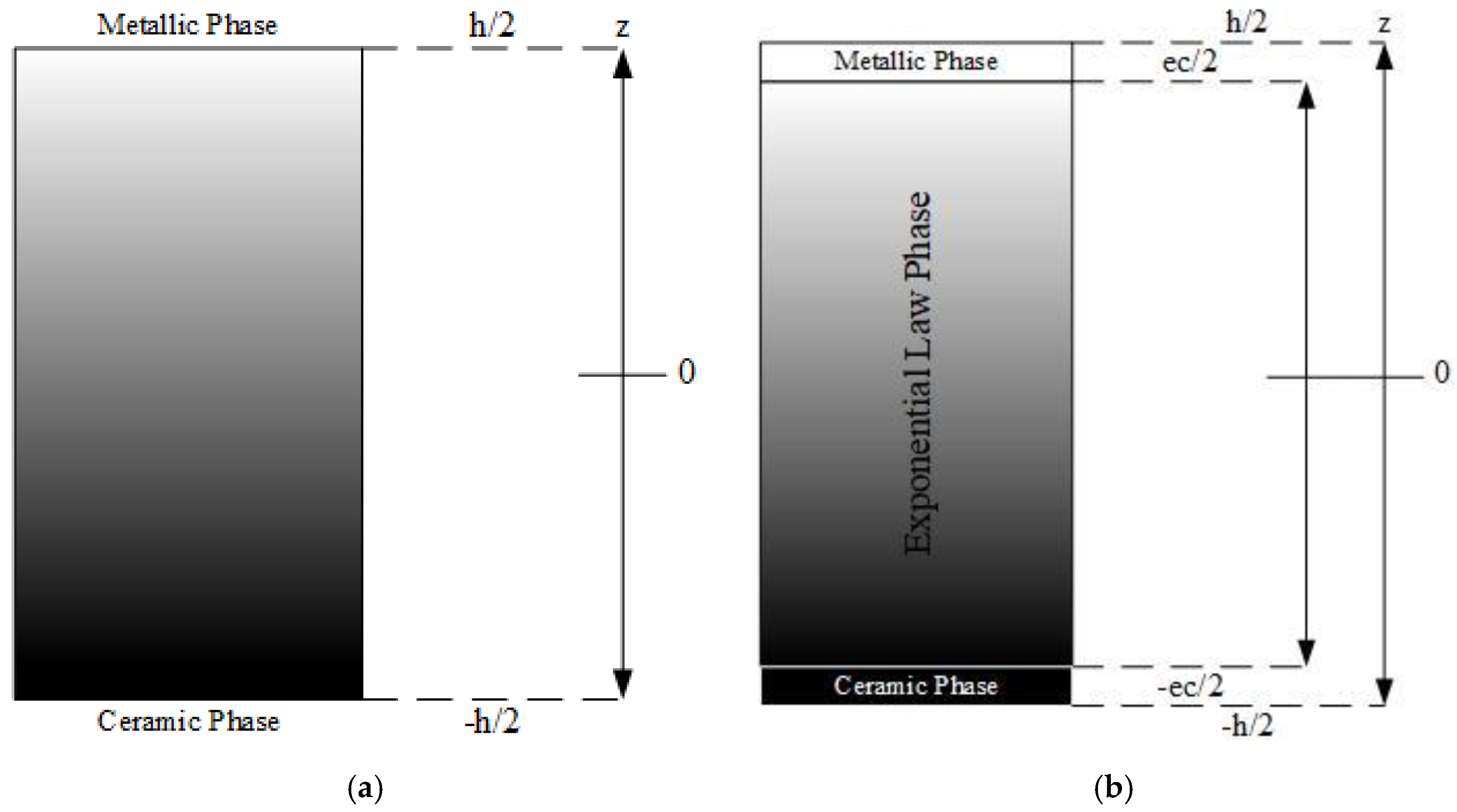
In the present study, one considers a dual-phase exponential law distribution (Bouchafa et al. [21], Bernardo et al. [22]) that resembles a sandwich, where the outer layers are constituted by the individual phases, and the core results from the phases’ exponentially graded mixture. In Figure 1, it is possible to observe the more commonly studied power exponent law distribution (Figure 1a) and the one considered in this study, the exponential law (Figure 1b), assuming that, as it is the case, one has a dual-phase metallic–ceramic FGM, with a through-thickness mixture variation.

In the power exponent law configuration, the volume fraction distribution of ceramic inclusions through the plate thickness h is presented in Equation (1) (Loja et al. [23]). Note that the thickness is associated with the z coordinate of the Cartesian reference system, and the xy plane is located at the plate mid-plane, which is being represented in Figure 1 by the null z coordinate.

$$V_c\left(z\right)={\left(\frac{1}{2}+\frac{z}{h}\right)}^p$$

(1)

where V_c denotes the volume fraction of the ceramic phase, and p denotes the exponent. Based on a selected distribution law, the material properties can be determined using Voigt’s rule of mixtures, among other possible homogenization schemes:

$$P\left(z\right)=\left(P_c-P_m\right)V_c\left(z\right)+P_m$$

(2)

with $P, P_c,P_m$ standing for any material property associated respectively to the graded composite, the ceramic phase, and the metallic phase, for instance the elasticity modulus $\left(E\right)$ and the Poisson’s ratio $\mathsf{\nu }$. The subscripts m and c denote the metallic and the ceramic phases of the FGM, respectively.

As previously mentioned, this work is focused on the exponential law configuration, whose constitution resembles a sandwich. According to Figure 1, this FGM has its top and bottom layers made exclusively from its metallic and ceramic phases, i.e., there is no mixture of these two phases on the outer layers. On the contrary, on the middle layer, there is a dual-phase FGM following an exponential distribution; the mathematical representation is expressed as follows:

$$\begin{array}{c}P\left(z\right)=P_c\hspace{1em}for\hspace{0.17em}-\frac{h}{2}\le z\le -\frac{ec}{2}\\ P\left(z\right)=A_1{e}^{B_1\left(ec-2z\right)}\hspace{1em}for\hspace{0.17em}-\frac{ec}{2}\le z\le \frac{ec}{2}\\ P\left(z\right)=P_m\hspace{1em}for\hspace{0.17em}\frac{ec}{2}\le z\le \frac{h}{2}\end{array}$$

(3)

with $A_1=P_m$ and $B_1=\frac{1}{2ec}\ln \left(\frac{P_c}{P_m}\right)$. The parameter (ec) denotes the FGM middle layer thickness and h denotes the total plate thickness, as can be observed in Figure 1b. As mentioned, $P$ represents a generic material property of the FGM, namely the elasticity modulus and the Poisson’s ratio.

2.2. Displacement Field and Constitutive Relation

Considering the plates’ characteristics that will be studied, both from the perspective of their aspect ratio and from the influence of the shear effects that should not be neglected, the present work is based on the first-order shear deformation theory (FSDT), in which the displacement field is given as (Mindlin [24] and Reissner [25]):

$$\{\begin{array}{c}u\left(x,y,z\right)=u^0\left(x,y\right)+z{\theta }_x^0\left(x,y\right)\\ v\left(x,y,z\right)=v^0\left(x,y\right)+z{\theta }_y^0\left(x,y\right)\\ w\left(x,y\right)=w^0\left(x,y\right)\end{array}$$

(4)

with $u^0, v^0$, and $w^0$ denoting the mid-plane displacements along the directions $x,y,z$ of a three-dimensional (3D) Cartesian system, and ${\theta }_x^0$ and ${\theta }_y^0$ standing for the rotations around the $y$ and $x$ axes, respectively. Considering the kinematical relations from elasticity theory for small deformations, and omitting dependencies, yields the linear strains’ displacement:

$$\begin{array}{c}\{\begin{array}{c}{\epsilon }_x^{}={\epsilon }_x^0+z{k}_x^0\\ {\epsilon }_y^{}={\epsilon }_y^0+z{k}_y^0\\ {\gamma }_{xy}^{}={\gamma }_{xy}^0+z{k}_{xy}^0\end{array}; \{\begin{array}{c}{\gamma }_{yz}^{}={\gamma }_{yz}^0\\ {\gamma }_{xz}^{}={\gamma }_{xz}^0\end{array}\\ \left\{\begin{array}{c}{\epsilon }_x^0\\ {\epsilon }_y^0\\ {\gamma }_{xy}^0\end{array}\right\}=\left\{\begin{array}{c}\frac{\partial u^0}{\partial x}\\ \frac{\partial v^0}{\partial y}\\ \frac{\partial u^0}{\partial y}+\frac{\partial v^0}{\partial x}\end{array}\right\};\left\{\begin{array}{c}{k}_x^0\\ k_y^0\\ k_{xy}^0\end{array}\right\}=\left\{\begin{array}{c}\frac{\partial {\theta }_x^0}{\partial x}\\ \frac{\partial {\theta }_y^0}{\partial y}\\ \frac{\partial {\theta }_x^0}{\partial y}+\frac{\partial {\theta }_y^0}{\partial x}\end{array}\right\}; \left\{\begin{array}{c}{\gamma }_{yz}^0\\ {\gamma }_{xz}^0\end{array}\right\}=\left\{\begin{array}{c}\frac{\partial w^0}{\partial y}+{\theta }_y^0\\ \frac{\partial w^0}{\partial x}+{\theta }_x^0\end{array}\right\}\end{array}$$

(5)

The relation of these strains to the corresponding state of stress is given by a constitutive relation based in the assumption that although macroscopically heterogeneous, these functionally graded composites can be considered isotropic at each point. Therefore, the constitutive equations are given as:

$$\begin{array}{c}\left\{\begin{array}{c}{\sigma }_x\\ {\sigma }_y\\ {\sigma }_{xy}\end{array}\right\}=\frac{E\left(z\right)}{1-\mathsf{\nu }{\left(z\right)}^2}\left[\begin{array}{ccc}1& \mathsf{\nu }\left(z\right)& 0\\ \mathsf{\nu }\left(z\right)& 1& 0\\ 0& 0& \frac{1-\mathsf{\nu }\left(z\right)}{2}\end{array}\right] \left\{\begin{array}{c}{\epsilon }_x^0+z{k}_x^0\\ {\epsilon }_y^0+z{k}_y^0\\ {\gamma }_{xy}^0+z{k}_{xy}^0\end{array}\right\}\\ \left\{\begin{array}{c}{\sigma }_{yz}\\ {\sigma }_{xz}\end{array}\right\}=\frac{E\left(z\right)}{2\left(1+\mathsf{\nu }\left(z\right)\right)}\left[\begin{array}{cc}1& 0\\ 0& 1\end{array}\right]\left\{\begin{array}{c}{\gamma }_{yz}^0\\ {\gamma }_{xz}^0\end{array}\right\}\end{array}$$

(6)

where the thickness coordinate dependence arising from the exponential law is visible at the elastic stiffness membrane-bending and shear coefficients matrices.

The finite element linear static analyses performed are governed by the usual equilibrium equation (Equation (7)) after the imposition of the adequate set of boundary conditions (Zienckiewickz et al. [26]):

$$\mathit{K}\mathit{q}=\mathit{f}$$

(7)

where $\mathit{K}, \mathit{q}, \mathit{f}$ stand respectively for the global stiffness matrix, the generalized nodal displacements vector, and the generalized forces vector. The implemented FSDT-based finite element code considered nine-node quadrilateral plate elements (Q9, Lagrange family). A selective integration scheme was considered with a shear correction factor of 5/6, in order to minimize the shear locking effects (Loja et al. [27], Reddy [28]).

2.3. Uncertain Material and Geometrical Properties

The existing response variability of real FGM plates was simulated by assuming that each material and geometrical characteristic property is affected by uncertainty.

As the focus of the present study is the static response of dual-phase exponential law FGM plates, we will direct our study to the input parameters’ uncertainty simulation. These input parameters, also denoted by model parameters, are constituted by the phases’ material properties and layers’ thicknesses.

As each model parameter will have a specific influence on the simulated static response, and therefore on the characterization of its variability, this study considers a random multivariate normal distribution to simulate the uncertainty associated with those parameters. Therefore, the parameters were sampled considering that X∼N(μ,Σ), i.e., X is a multivariate normal distribution with the mean value μ and the covariance matrix Σ. As one wants to ensure the independence between modeling parameters, the covariance matrix Σ will be a diagonal matrix. To this purpose, taking into account the ability to ensure the independence between variables (Iman and Conover [29]), this study uses a Latin hypercube sampling (LHS) technique (Beck and Santos [30]).

2.4. Multiple Linear Regression Model

Aiming to obtain a set of non-deterministic models to relate multiple variables with an expected response result, this study considers a statistical classical approach, assuming that, for a generic problem, such variables will follow a linear relation, as:

$$Y={\beta }_0+{\beta }_1{X}_1+\dots +{\beta }_k{X}_k+ϵ$$

(8)

where $k$ denotes the number of independent input parameters, ${\beta }_0$ is the zero intercept, ${\beta }_k$ is the predictor slope for the k-th variable, $X_k$ is the k-th input parameter variable, $Y$ is the real response of the model, and $ϵ$ is the Gaussian error term.

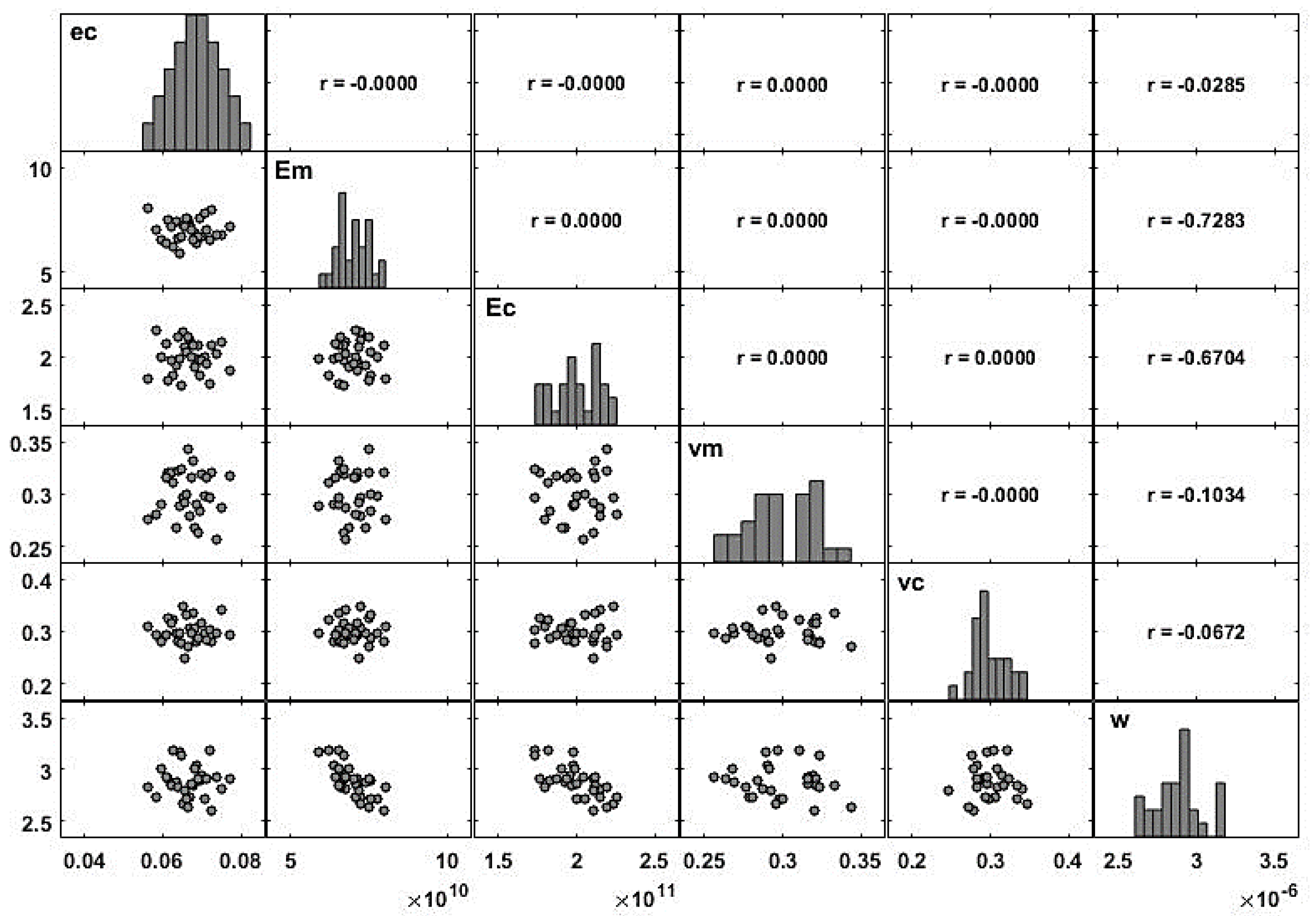
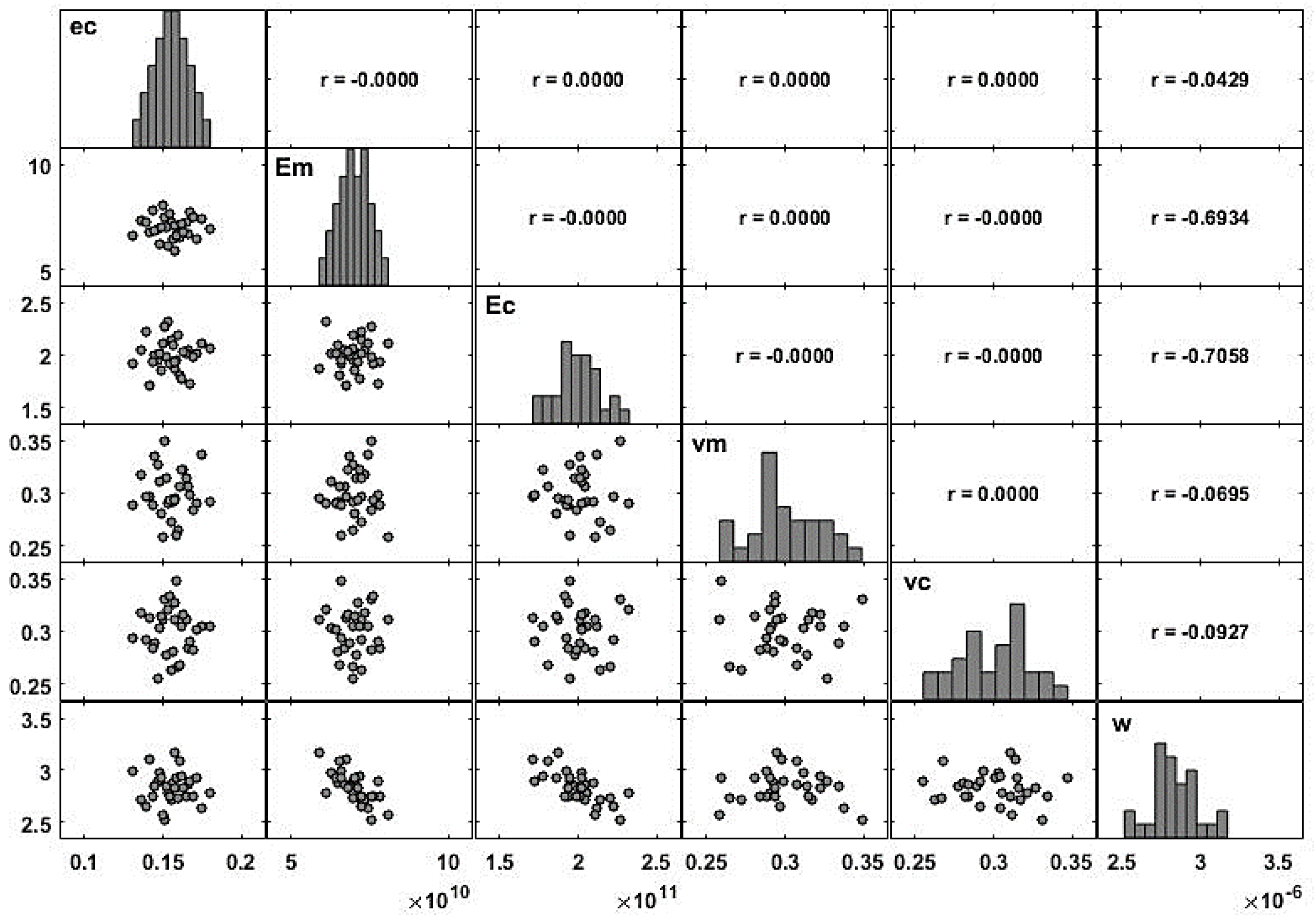
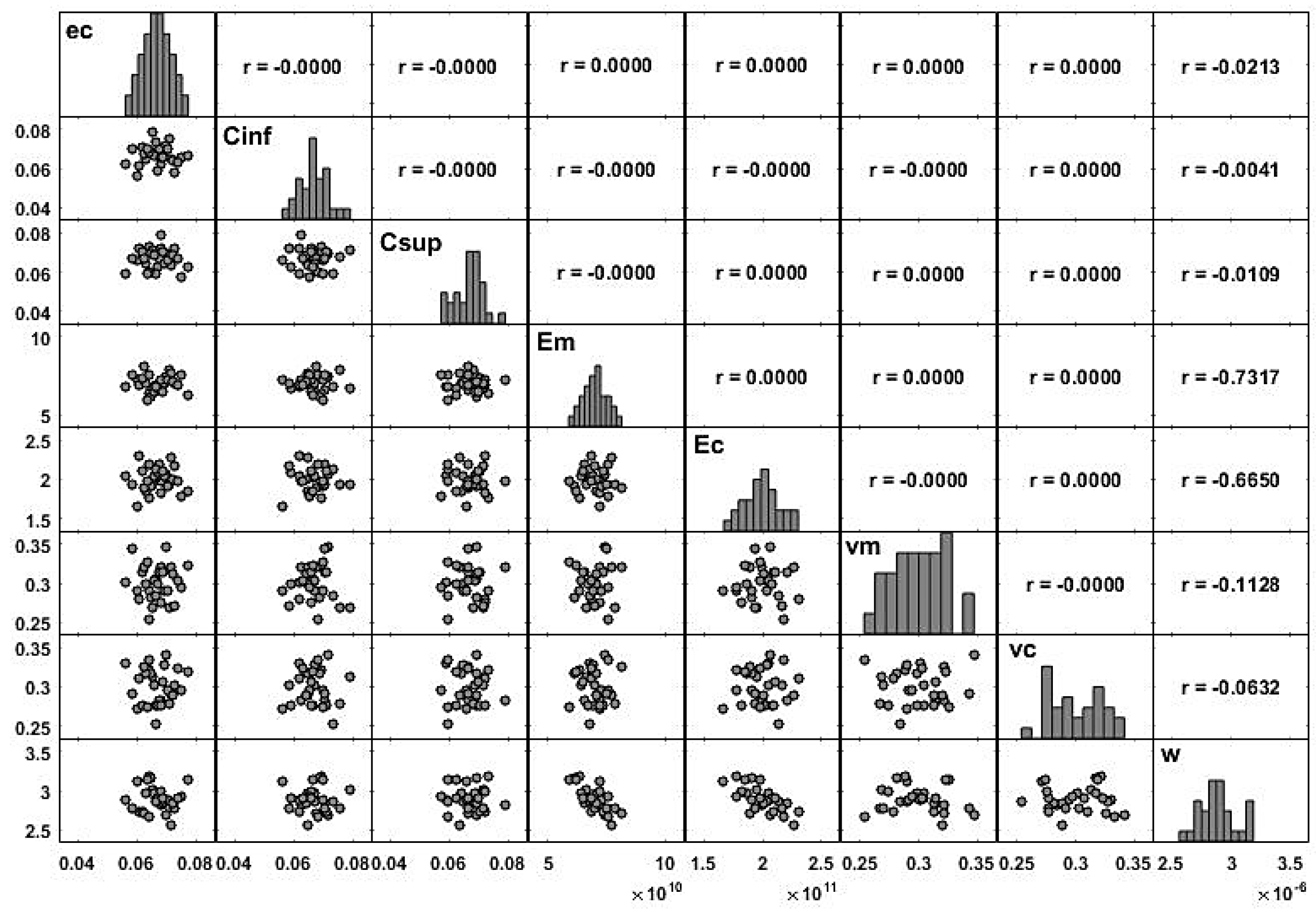
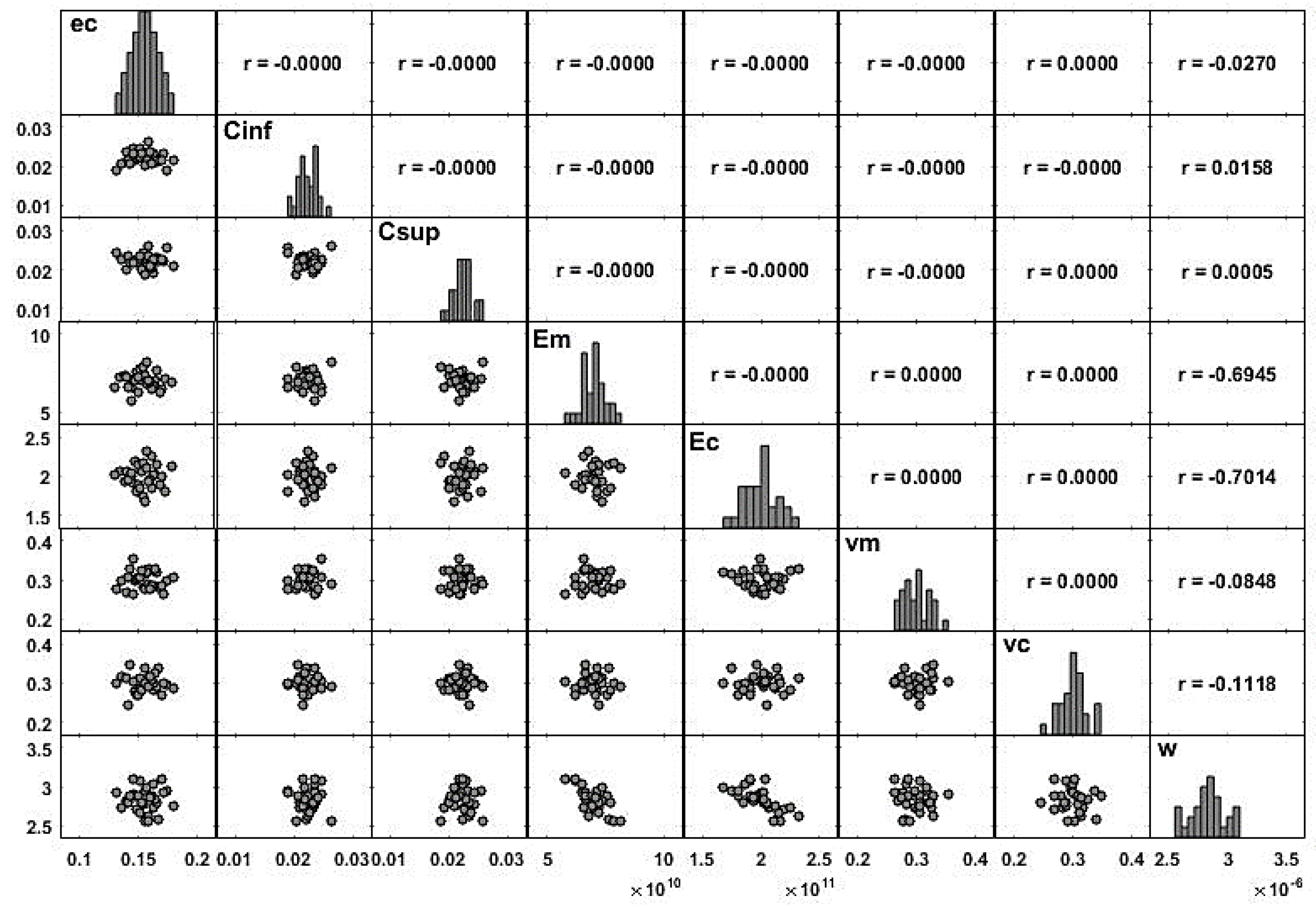
When there is more than one variable defined on a probability space, it is important to understand the relation between the random variables that are involved. A common measure of the linear relation between two random variables is the covariance (denoted in this sub-section by ${\sigma }_{XY}$) which is given as ${\sigma }_{XY}=cov\left(X,Y\right)=E\left[\left(X-{\mu }_X\right) \left(Y-{\mu }_Y\right)\right]$. The covariance measures the linear relation between two variables but depends on the magnitude of the variables. So, it is common to scale the covariance by the standard deviation of each variable (denoted in this sub-section by ${\sigma }_X, {\sigma }_Y$), which leads to the correlation, ${\rho }_{XY}=\frac{{\sigma }_{XY}}{{\sigma }_X{\sigma }_Y}$. This measure can be used for comparison purposes, as it is easier to analyze. For any pair of variables $\left(X,Y\right)$, the correlation ranges between $-1\le {\rho }_{XY}\le 1$, and a null coefficient means that the variables are not linearly correlated. If this coefficient is close to 1 (or $-1$), the two variables are linearly correlated in the positive (or negative) direction. In order to avoid multicollinearity problems, the model requires independence of the input variables, which is ensured by the use of the LHS technique. This independence can be easily verified through the correlation coefficients between the samples of the input variables.

Sometimes, it is necessary to include the interaction effects in the multiple linear regression (MLR) methods, which will be represented, if necessary, by a cross-product term in the model, such as $Y={\beta }_0+{\beta }_1{X}_1+{\beta }_k{X}_k+{\gamma }_{12}{X}_1{X}_2+ϵ$.

The model may also be represented using matrix notation. In such case, for k independent variables and n observations, (x_i1, x_i2, …, x_in), i = 1, 2, …, n, and the dependent variable, one has:

$$y_{\mathrm{i}}={\beta }_0+{\beta }_1{x}_{\mathrm{i}1}+{\beta }_2{x}_{\mathrm{i}2}+\dots +{\beta }_k{x}_{ik}+{ϵ}_{\mathrm{i}}, i=1,2,\dots ,n.$$

(9)

This model is a system with n equations, which can be expressed as:

$$\mathit{y}=\mathit{X}\mathit{\beta }+\mathit{ϵ},$$

where:

$$\mathit{y}=\left[\begin{array}{c}{y}_1\\ y_2\\ ⋮\\ y_n\end{array}\right],\mathit{X}=\left[\begin{array}{ccccc}1& x_{11}& x_{12}& \cdots & x_{1k}\\ 1& x_{21}& x_{22}& \cdots & x_{1k}\\ ⋮& ⋮& ⋮& \ddots & ⋮\\ 1& x_{n1}& x_{n2}& \cdots & x_{1k}\end{array}\right],\mathit{\beta }=\left[\begin{array}{c}{\beta }_0\\ {\beta }_1\\ ⋮\\ {\beta }_k\end{array}\right],\mathrm{and}\mathit{ϵ}=\left[\begin{array}{c}{ϵ}_1\\ {ϵ}_2\\ ⋮\\ {ϵ}_n\end{array}\right].$$

The residuals describe the error in the fit of the model to the observations. The acceptance of the model requires the residuals to be independent, normally distributed, with null average, and with constant standard deviation, i.e., $\mathit{ϵ}$∼N(0,σ²). If the assumptions of this model are verified, a response prediction $\widehat{y}$ can be estimated via the least squares method from the sampled values.

For a descriptive study, the correlation coefficient between two samples, $\left(x_1,\dots ,x_n\right)$ and $\left(y_1,\dots ,y_n\right),$ can be defined as $r_{xy}=\frac{{{\displaystyle \sum }}_{i=1}^n\left(x_i-\overline{x}\right)\left(y_i-\overline{y}\right)}{\sqrt{{{\displaystyle \sum }}_{i=1}^n{\left(x_i-\overline{x}\right)}^2{{\displaystyle \sum }}_{i=1}^n{\left(y_i-\overline{y}\right)}^2}}$. Using some data, it is possible to estimate a multiple linear regression model defined according to Equation (9), and the contribution of each regressor is estimated through the regression coefficients ${\beta }_k$.

Also, in order to assess the quality of the model, the coefficient of multiple determination, $R^2$, or the adjusted $R^2$ (Adj-R²) can be used. These coefficients are global statistics and provide a measure of the percentage of variability of the dependent variable that is explained by the model (for details, see Montgomery [31]).

For an inferential study, the sampled results can be generalized to the population. With the analysis of variance (ANOVA), one can test the significance of the model based on the p-value of the F-test (Montgomery [31]). The idea is to divide the total variability of the response variable into meaningful components; i.e., the total sum of squares, $SST={\displaystyle \sum }_{i=1}^n{\left(y_i-\overline{y}\right)}^2$, is partitioned into a sum of squares due to regression, $SSE={\displaystyle \sum }_{i=1}^n{\left({\widehat{y}}_i-\overline{y}\right)}^2$, and a sum of squares due to error, $SSR={\displaystyle \sum }_{i=1}^n{\left({\widehat{y}}_i-\overline{y}\right)}^2$,

$$SST=SSE+SSR.$$

For a given significant level α (usually 5%), if the null hypothesis is rejected, the model is significant (p-value ≤ α). In those cases, at least one of the slopes is non-zero. Under these conditions, the t-test gives the significance of each individual independent variable or model parameter (Montgomery [31]).

For simplicity, usually the linear regression model (LRM) output displays significant codes for the different p-values: from the most significant p-value ≅ 0 (‘***’), 0.001 (‘**’), 0.01 (‘*’), 0.05 (‘.’), to the less significant 0.1 (‘·’). Frequently, the higher significant level is 10%; above this value, the null hypothesis is not rejected, and the model (F-test) or coefficient (t-test) is not significant. With these partial results, it is possible to build new models with the most significant regressors. Moreover, it is possible to construct confidence intervals for the partial slopes.

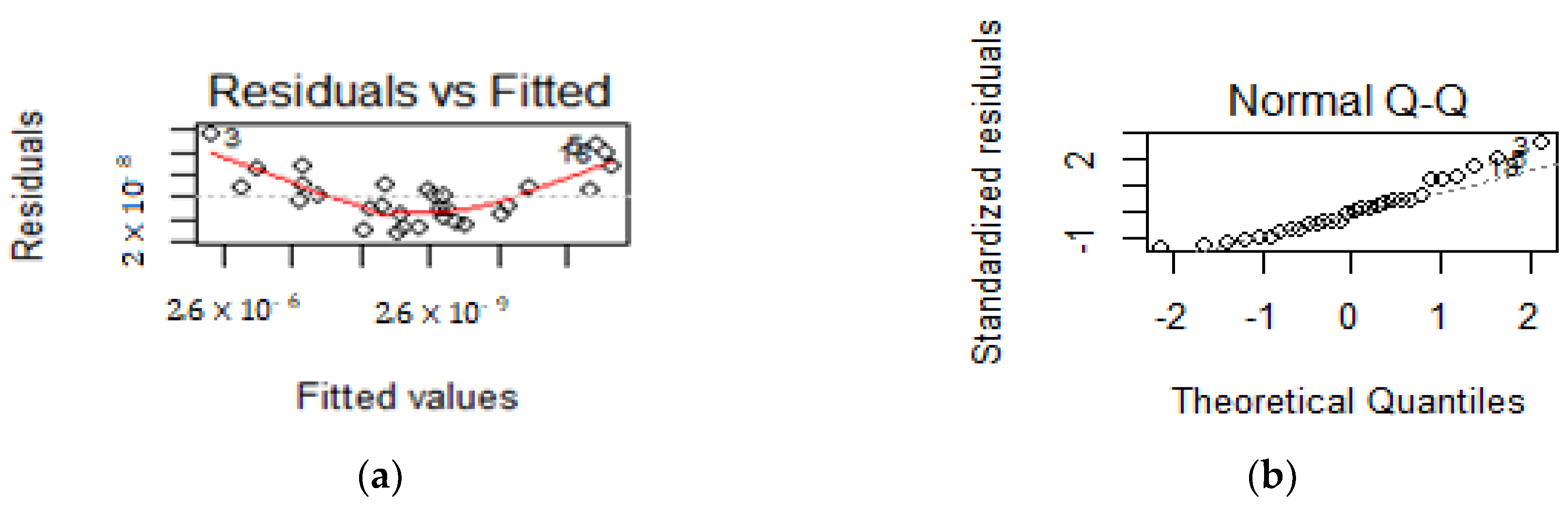
Once the model is chosen, one has to be sure of the validity of the model, namely on the residuals’ assumptions. To validate the null average of the residual, one can use the usual hypothesis testing for the mean (Montgomery [31]). The normality assumption can be visually checked by a normal quantile–quantile plot (NQQP) or a normal probability plot (NPP), and confirmed with a goodness of fit test, such as the Kolmogorov–Smirnov test (Montgomery [31]). To check the other two assumptions (independence and equal variance), one can inspect the plot of the residuals against the fitted values. If a pattern appears, it means that there is no independence of the residuals; so, the independence assumption isn’t validated. Also, if the same plot suggests non-constant variance along the fitted values, the variance homoscedasticity is not guaranteed (Montgomery [31]). In such circumstances, another model should be considered.

3. Numerical Applications

3.1. Verification Cases

As a first case study, and to ensure the quality of the subsequent results, one proceeded to a preliminary verification of the finite element code that was developed and implemented. To this purpose, two material phases were considered: aluminum (E_m = 70 GPa, ν_m = 0.3) and zirconia (E_c = 200 GPa, ν_c = 0.3), yielding its graded mixture, an AlZrO₂ FGM. The static behavior of the FGM simply supported plate was compared with Bernardo et al. [22].

In Figure 2, it is possible to observe the coordinate system used and the plate position associated with it. The transverse uniform pressure loading is also visible, as well as the simply supported borders denoted by the dashed lines in the top view (Szilard [32]). To reproduce the exact simulation conditions, a discrete approach with 25 layers was adopted. The effective properties associated with each layer were determined considering the corresponding values using the power exponent law at each layer’s mid-height, and further, the Voigt rule.

The plate domain was discretized using $17\times 17$ Lagrangian four node elements (Q4) and nine node elements (Q9), and the plate was submitted to a constant unit pressure of ${10}^4\mathrm{Pa}$. The study was conducted for three aspect ratios ($a/h=5, 10, \mathrm{and} 20$, where ($a$) is the plate edge dimension ($a=1\mathrm{m}$), and ($h$) stands for the thickness. The power exponent $p$ used, was $7$. The results obtained are presented in

Table 1. Non-dimensional maximum deflection $w_{ndim}$ and deviation. Power law functionally graded materials (FGM).

a/h	Models	${\mathit{w}}_{\mathit{n}\mathit{d}\mathit{i}\mathit{m}}$$\mathbf{(}\mathbf{\times }{\mathbf{10}}^{\mathbf{-}\mathbf{6}}\mathbf{)}$	$\mathit{D}\mathit{e}\mathit{v} (\%)$
5	Bernardo et al. [22]	2.282	-
	Present Q4	2.264	0.789
	Present Q9	2.280	0.088
10	Bernardo et al. [22]	3.187	-
	Present Q4	3.168	0.596
	Present Q9	3.194	0.220
20	Bernardo et al. [22]	4.913	-
	Present Q4	4.887	0.529
	Present Q9	4.920	0.142

in a non-dimensional form using the multiplier $w_{ndim}=w_{max}/h$, where $w_{max}$ is the maximum deflection.

The deviations were determined according to $dev(\%)=\left|\frac{w_{present}-w_{ref}}{w_{ref}}\right|\times 100\%$. From Table 1, it is possible to conclude on the good agreement between the present models and the reference results, particularly for the Q9 model, which provides the minor deviations for all of the aspect ratios. Considering these results, and although the deviations presented by Q4 are quite acceptable, one will proceed with the Q9 model for the subsequent cases.

A second verification case was performed, now considering a simply supported FGM plate whose configuration is described by the exponential law (Figure 1b). The aim of this case was to assess the influence of the core thickness to the total thickness ratio (ec/h), thus being considered three values for this relation, as presented in

Table 2. Non-dimensional maximum deflection $w_{ndim}$ and deviation. Exponential law FGM.

a/h	ec/h	${\mathit{w}}_{\mathit{n}\mathit{d}\mathit{i}\mathit{m}}$$\mathbf{(}\mathbf{\times }{\mathbf{10}}^{\mathbf{-}\mathbf{6}}\mathbf{)}$		Dev (%)
		Bernardo et al. [22]	Present Q9
5	1/3	2.874	2.874	0
	2/3	2.834	2.834	0
	7/9	2.826	2.823	0.106
10	1/3	4.082	4.074	0.196
	2/3	4.003	3.995	0.199
	7/9	3.986	3.971	0.376

with the corresponding results.

From Table 2, it is also possible to conclude on the good agreement between the reference and the Q9 model in the present verification case. Concerning the mentioned ratio evolution trend, we observe that as the ratio increases, and therefore the FGM layer increases (simultaneously decreasing the outer layers thicknesses), the non-dimensional deflection decreases.

3.2. Case Studies

This sub-section considers a set of case studies focused on FGM plates whose constitution is ruled by the exponential law configuration.

The first case study aimed to analyze the influence of the FGM layer thickness on the maximum deflection of the plate, while maintaining the total plate thickness so that the outer layers thicknesses will be given as half the remaining value of the constant total thickness. In the second case study, assuming that all of the layers may be individually affected by uncertainty, one assesses the impact that this may have to the plate response. In both cases, it is additionally considered that the material properties will be affected by variability.

To perform these studies, one has maintained the discrete approach used in the verification cases, which enables not only achieving a good approximation to the continuous variation, but also allows a better approximation to real manufacturing processes. The plates continue to maintain all of their borders as simply supported, being considered an aspect ratio $a/h=5$. All of the plates are submitted to a ${10}^4\mathrm{Pa}$ uniformly distributed load. The statistical results were obtained through the programming of a statistical computing environment platform (“The R Project for Statistical Computing”, 2018 [33]).

3.2.1. Uncertainty in the Material Properties and FGM Core Thickness

In this first case, one studied two relations of core to total thicknesses ($ec/h$). Following the second verification case in Section 3.1 and aiming at considering the limit values of the core to the total thickness ratios range, the present work considered the ratios 1/3 and 7/9. The uncertainty associated with the thickness of the core was simulated according to a normal distribution as referred in Section 2.3.

• Thinner Core (ec/h = 1/3)

The average material properties used in the present study are presented in

Table 3. Parameters mean values: case 3.2.1—Thinner core.

Properties	ec/hc	Em (GPa)	Ec (GPa)	νm	νc
μ (mean)	1/3	70	200	0.3	0.3

, assuming a normal distribution when generating the randomly generated vectors for each of the input parameters. As a measure of variability, a coefficient of variation of 7.5% was used, which gives a standard deviation that corresponds to 7.5% of the mean values (σ = 0.075 μ). This methodology was also applied in all of the subsequent models.

Figure 3 illustrates the correlations among the generated input material and geometrical parameters, as well as between them, and the maximum transverse deflection (w). As expected, one observes that the randomly generated input vectors present normal distributions as well as null correlation coefficients between the input variables. Also as expected, most of the histograms suggest normal distributions.

Only between the maximum deflection and the input parameters do non-null correlations occur. Considering the relative contribution that each material or geometrical parameter may have to the plate static response, one can conclude that there is a higher correlation between the maximum deflection ($w$) and the Young’s modulus of both material phases ($r_{w{E}_m}=-0.73$, $r_{w{E}_c}=-0.67$). It is also pertinent to consider that these two coefficients are affected by the minus sign, which reveals that the elasticity modulus of the different phases have an inverse correlation to the maximum deflection. From a global analysis concerning each variable contribution, one can say that the variability of the maximum transverse deflection is mostly explained by the Young’s modulus of the two material phases.

The possibility of achieving a regression model related to this case study, as for others, may constitute an important tool as an alternative model to the finite element method, as long as the analysis will be within the same domain of study. Thus, one has built for the present case a multiple linear regression model with all of the input variables, and one concluded that, except for the core thickness, all of the regressors are significant.

If one builds a model with all of the significant parameters (all except ec), one obtains a residual analysis showing that some of the assumptions are violated (independence and normality). As we may observe from Figure 4a, the obtained pattern suggests a quadratic dependence of the residual, as well as a non-normal behavior (Figure 4b) confirmed by the Kolmogorov–Smirnov goodness of fit test.

Globally, taking into account the results, we may say that the elasticity modulus of the two materials, E_m and E_c, have a higher contribution for the explanation of the transverse deflection ($w$) variability, being the most significant among all of the parameters.

Table 4. Regression Statistic: case 3.2.1—Thinner core.

LRM1	Coefficients	2.5% CI	97.5% CI	p-Value
Intercept	5.800 × 10−6	5.626148 × 10−6	5.974 × 10−6	<2 × 10−16 ***
Em	−2.157 × 10−17	−2.332488 × 10−17	−1.982 × 10−17	<2 × 10−16 ***
Ec	−7.021 × 10−18	−7.635766 × 10−18	−6.407 × 10−18	<2 × 10−16 ***

Residual standard error: 2.407 × 10⁻⁸ on 27 degrees of freedom (DF), Multiple R²: 0.9778, Adj-R^2: 0.9762, F-statistic: 594.6 on 2 and 27 DF, p-value: <2.2 × 10⁻¹⁶. Significant codes: 0 ‘***’, 0.001 ‘**’, 0.01 ‘*’, 0.05 ‘.’, 0.1 ‘·’, 1.

presents the results of a new model (Equation (9)) with just the two most significant parameters, namely E_m and E_c.

$$\widehat{w}=5.8\times {10}^{-6}-2.157\times {10}^{-17}{E}_m-7.021\times {10}^{-18}{E}_c$$

(10)

This new model (LMR1) verified the residual assumptions. The normality assumption was also verified with the Komolgorov–Smirnov goodness of fit test, and the null mean was validated with the t-student test for the mean. From the R², one can also observe a very good fitting.

This simpler model (10) considering only the elasticity modulus of the two materials, Em and Ec, is able to explain 97.62% of the maximum deflection variability. To note the influence of the magnitude order of the different elasticity moduli reflected at the ${\beta }_k$ coefficients (Equations (8) and (10)).

• Thicker core (ec/h = 7/9)

In this second situation of the first case study, we have considered that the FGM core thickness would be predominant when compared to the previous situation. So, following the same methodology, one has generated a new set of random vectors using the same methodology that was already discussed. The average values for the material and geometrical properties are presented in

Table 5. Parameters mean values: case 3.2.1—Thicker core.

Properties	ec/h	Em (GPa)	Ec (GPa)	νm	νc
μ (mean)	7/9	70	200	0.3	0.3

, where the thickness ratio is now greater.

The null correlations among the generated input material and geometrical parameters are observed again in Figure 5, thus proving the input parameters’ independence. The correlations of these parameters to the maximum transverse deflection ($w$) is also shown. As it was concluded in the previous case study, the higher contribution of the Young’s modulus of both material phases is also visible here, when compared to the correlations of the remaining parameters to the plate response. They present again very similar values ($r_{w{E}_m}=-0.69$, $r_{w{E}_c}=-0.71$).

We can observe from Figure 3 and Figure 5 that in this latter case, the FGM layer thickness presents a higher value of correlation to the maximum deflection. However, it is still not relevant, the same being said for the Poisson’s ratios of the different materials.

In the sequence of this correlation analysis, one has built the corresponding multiple regression model, and all of the parameters were significant. Although this model provides a good fit, Adj-R² = 0.9934, the independence assumption of the residuals is violated.

Therefore, one has simplified the model using just the two most significant variables, E_m and E_c, yielding a new model (LMR2), which is now presented in Equation (11). This LMR2 model obtained via a multiple linear regression model verified the residues’ assumptions of normality, null mean, constant variance, and the residues’ independence requisites.

$$\widehat{w}=5.667\times {10}^{-6}-2.003\times {10}^{-17}{E}_m-7.162\times {10}^{-18}{E}_c$$

(11)

The regression statistics data corresponding to this model (Equation (11)) is presented in

Table 6. Regression statistic for the second study: case 3.2.1—Thicker core.

LRM2	Coefficients	2.5% CI	97.5% CI	p-Value
Intercept	5.677 × 10−6	5.501 × 10−6	5.834 × 10−6	<2 × 10−16 ***
Em	−2.003 × 10−17	−2.171 × 10−17	−1.835 × 10−17	<2 × 10−16 ***
Ec	−7.162 × 10−18	−7.750 × 10−18	−6.574 × 10−18	<2 × 10−16 ***

Residual standard error: 2.305 × 10⁻⁸ on 27 degrees of freedom, Multiple R²: 0.9784, Adj-R²: 0.9768, F-statistic: 611.6 on 2 and 27 DF, p-value: <2.2 × 10⁻¹⁶. Significant codes: 0 ‘***’, 0.001 ‘**’, 0.01 ‘*’, 0.05 ‘.’, 0.1 ‘·’, 1.

.

This simplified model (Equation (11)), which accounts for the influence of both elasticity modulus, E_m and E_c, is able to explain 97.68% of the maximum deflection variability. Again, the coefficients associated with each elasticity modulus reflected their different mean magnitude order.

3.2.2. Uncertainty in the Material Properties and Whole Sandwich Thickness

In this second case study, we looked at the FGM plate thickness from a different perspective. Now, contrarily to the study developed in Section 3.2.1, it is considered that all of the layers’ thicknesses may be independently affected by uncertainty, thus varying the plate’s total thickness. To ease the cases reference, one maintains the same terminology (thinner core and thicker core).

• Thinner Core (ec/h = 1/3)

As in the previous cases, a normal distribution was assumed when generating the random vectors for each of the input parameters, which now include the thicknesses of the three layers. The average material properties are presented in

Table 7. Parameters mean values: case 3.2.2—Thinner core.

Properties	ec/h	Cinf/h	Csup/h	Em (GPa)	Ec (GPa)	νm	νc
μ (mean)	1/3	1/3	1/3	70	200	0.3	0.3

, and one has considered a standard deviation that corresponds to 7.5% of the mean values.

The correlations among the generated input parameters are presented in Figure 6, as well as between these and the maximum transverse deflection (w). The null correlation among the input parameters and their histograms with a normal-like configuration is an expected result.

From the correlation matrix plot in Figure 6, one can observe that there is a higher correlation between the Young’s modulus properties of both phases ($r_{w{E}_m}=-0.73$, $r_{w{E}_c}=-0.67$) and the maximum deflection ($w$) when compared with the other parameters. It is relevant to note from the results obtained so far that in this type of exponentially graded material, the thickness of the plate does not present a high correlation value, contrarily to that happening in the power law configuration (Carvalho et al. [19]).

One proceeded next to the multiple regression model construction. In this model, all of the parameters were significant, with the exception of the geometrical properties and the thicknesses (ec, Cinf, and Csup). Although this model provides a good fit with Adj-R² = 0.9921, the independence assumption of the residuals was violated. Therefore, a new model (LMR3) with just the elasticity modulus of the two materials, E_m and E_c, was built. This new model provided a good fit, Adj-R² = 0.9748, and the residual assumptions were verified.

Table 8. Regression statistic: case 3.2.2—Thinner core.

LMR3	Coefficients	2.5% CI	97.5% CI	p-Value
Intercept	5.801 × 10−6	5.622 × 10−6	5.984 × 10−6	<2 × 10−16 ***
Em	−2.178 × 10−17	−2.359 × 10−17	−1.997 × 10−17	<2 × 10−16 ***
Ec	−6.958 × 10−18	−7.591 × 10−18	−6.326 × 10−18	<2 × 10−16 ***

Residual standard error: 2.43 × 10⁻⁸ on 26 degrees of freedom, Multiple R²: 0.9765, Adj-R²: 0.9748, F-statistic: 560.8 on 2 and 27 DF, p-value: <2.2 × 10⁻¹⁶. Significant codes: 0 ‘***’, 0.001 ‘**’, 0.01 ‘*’, 0.05 ‘.’, 0.1 ‘·’, 1.

presents the results of this model (Equation (12)) with just the two most significant parameters (E_m and E_c).

$$\widehat{w}=5.801\times {10}^{-6}-2.178\times {10}^{-17}{E}_m-6.958\times {10}^{-18}{E}_c$$

(12)

Table 8 presents the regression statistic information associated with the present model (Equation (12)).

This simplified model (LMR3) verified the residuals’ assumptions. The normality assumption was also verified with the Komolgorov–Smirnov goodness of fit test, and the null mean was validated with the t-student test for the mean.

• Thicker Core (ec/h = 7/9)

The final situation in this case study is related to the thicker core configuration. As previously, a normal distribution was assumed when generating the randomly generated vectors for each of the input parameters. The average material properties are presented in

Table 9. Parameters mean values: case 3.2.2—Thicker core.

Properties	ec/h	Cinf/h	Csup/h	Em (GPa)	Ec (GPa)	νm	νc
μ (mean)	7/9	1/9	1/9	70	200	0.3	0.3

, and again, one has considered a standard deviation that corresponds to 7.5% of the mean values.

The randomly generated input vectors were analyzed for their correlation to ascertain the independence between them. The results obtained are presented in Figure 7. We can see that there is no correlation between the inputs, as expected.

From Figure 7, we concluded that also for this case, the parameters that presented higher correlations to the maximum transverse deflection were the metallic and ceramic elasticity moduli ($r_{w{E}_m}=-0.69$, $r_{w{E}_c}=-0.70$).

In terms of a global model for this case, one has started by considering the use of all of the input variables, but again, the geometrical parameters, ec, Cinf and Csup, were not significant. Although the fit was very good, the independence assumption was rejected, as well as the normality of the residuals.

Using just the elasticity modulus of the two materials (E_m and E_c), another multiple linear regression model (LRM4) was built (

Table 10. Regression statistic: case 3.2.2—Thicker core.

LMR4	Coefficients	2.5% CI	97.5% CI	p-Value
Intercept	5.661 × 10−6	5.479 × 10−6	5.844 × 10−6	<2 × 10−16 ***
Em	−2.024 × 10−17	−2.209 × 10−17	−1.840 × 10−17	<2 × 10−16 ***
Ec	−7.052 × 10−18	−7.697 × 10−18	−6.406 × 10−18	<2 × 10−16 ***

Residual standard error: 2.53 × 10⁻⁸ on 27 degrees of freedom, Multiple R²: 0.974, Adj-R²: 0.972, F-statistic: 505.2 on 2 and 27 DF, p-value: <2.2 × 10⁻¹⁶. Significant codes: 0 ‘***’, 0.001 ‘**’, 0.01 ‘*’, 0.05 ‘.’, 0.1 ‘·’, 1.

), and the residuals’ assumptions of normality, null mean, constant variance, and independence were then verified.

$$\widehat{w}=5.661\times {10}^{-6}-2.024\times {10}^{-17}{E}_m-7.052\times {10}^{-18}{E}_c$$

(13)

From an analysis of Table 10 and establishing a comparison with the previous cases, we conclude that the results are similar. Both the elasticity moduli are equally significant, and the ${\beta }_k$ coefficients reflect the influence of these material properties to the plate static response.

3.2.3. Verification of Statistic Models

To verify the different statistic models obtained, a new random vector of material properties was generated and introduced in the statistical models. The values of the maximum transverse displacements obtained were compared to the values obtained from the finite element method (FEM) code as represented in

Table 11. Verification of statistic model LRM1 (case study 1, thinner core).

ec	Em	Ec	νm	νc	w(FEM)	w(LRM1) (Equation (10))	$\mathit{D}\mathit{e}\mathit{v}$ $\mathbf{(}\mathbf{\%}\mathbf{)}$
0.067	6.32 × 1010	1.83 × 1011	0.298	0.300	3.17 × 10−6	3.15 × 10−6	−0.63
0.073	7.40 × 1010	1.96 × 1011	0.320	0.290	2.80 × 10−6	2.83 × 10−6	1.07
0.060	7.56 × 1010	1.92 × 1011	0.298	0.290	2.82 × 10−6	2.82 × 10−6	0.00
0.064	6.67 × 1010	2.19 × 1011	0.320	0.300	2.81 × 10−6	2.82 × 10−6	0.36
0.069	7.05 × 1010	2.10 × 1011	0.269	0.300	2.82 × 10−6	2.805 × 10−6	−0.53

,

Table 12. Verification of statistic model LRM2 (case study 1, thicker core).

ec	Em	Ec	νm	νc	w(FEM)	w(LRM2) (Equation (11))	$\mathit{D}\mathit{e}\mathit{v}$ $\mathbf{(}\mathbf{\%}\mathbf{)}$
0.162	6.35 × 1010	2.11 × 1011	0.317	0.300	2.87 × 10−6	2.89 × 10−6	0.70
0.141	6.68 × 1010	1.85 × 1011	0.297	0.300	3.02 × 10−6	−2.66 × 10−6	−1.88
0.171	7.05 × 1010	1.88 × 1011	0.280	0.290	2.91 × 10−6	−2.76 × 10−6	−1.95
0.156	7.67 × 1010	1.97 × 1011	0.326	0.300	2.70 × 10−6	−2.95 × 10−6	−2.09
0.162	6.35 × 1010	2.11 × 1011	0.319	0.300	2.87 × 10−6	−2.783 × 10−6	−1.97

,

Table 13. Verification of statistic model LRM3 (case study 2, thinner core).

ec	Cinf	Csup	Em	Ec	νm	νc	w(FEM)	w(LRM3) (Equation (12))	$\mathit{D}\mathit{e}\mathit{v}$ $\mathbf{(}\mathbf{\%}\mathbf{)}$
0.070	0.0577	0.0636	7.1845 × 1010	1.7526 × 1011	0.285	0.285	3.036 × 10−6	3.017 × 10−6	−0.64
0.066	0.0644	0.0686	6.6026 × 1010	2.1604 × 1011	0.289	0.327	2.855 × 10−6	2.860 × 10−6	0.17
0.071	0.0726	0.0695	7.2244 × 1010	2.3191 × 1011	0.316	0.322	2.613 × 10−6	2.614 × 10−6	0.06
0.068	0.0685	0.0757	7.4522 × 1010	2.0961 × 1011	0.317	0.296	2.708 × 10−6	2.719 × 10−6	0.41
0.065	0.0677	0.0680	6.3931 × 1010	1.7996 × 1011	0.271	0.320	3.184 × 10−6	3.157 × 10−6	−0.87

and

Table 14. Verification of statistic model LRM4 (case study 2, thicker core).

ec	Cinf	Csup	Em	Ec	νm	νc	w(FEM)	w(LRM4) (Equation (13))	$\mathit{D}\mathit{e}\mathit{v}$ $\mathbf{(}\mathbf{\%}\mathbf{)}$
0.163	0.0213	0.0210	6.6935 × 1010	2.0556 × 1011	0.297	0.299	2.845 × 10−6	2.857 × 10−6	0.42
0.161	0.0238	0.02528	7.4074 × 1010	1.9224 × 1011	0.307	0.332	2.770 × 10−6	2.806 × 10−6	1.30
0.157	0.0225	0.0195	6.6448 × 1010	2.2384 × 1011	0.324	0.303	2.723 × 10−6	2.738 × 10−6	0.54
0.149	0.0225	0.0216	7.2553 × 1010	1.7789 × 1011	0.320	0.310	2.927 × 10−6	2.938 × 10−6	0.39
0.175	0.0242	0.0231	7.3403 × 1010	2.0808 × 1011	0.321	0.295	2.691 × 10−6	2.708 × 10−6	0.62

, for respectively the LRM1, LRM2, LRM3, and LRM4 models.

As one may conclude from Table 11, Table 12, Table 13 and Table 14, the deviations ($dev(\%)=\left|\frac{w_{present}-w_{ref}}{w_{ref}}\right|\times 100\%$) between each regression model and the finite element analysis results are very small. Therefore, each of the regression models that were developed may be considered as effective alternative calculation tools to be used instead of the finite element method, if the cases to be evaluated fall within the study domain.

4. Conclusions

The characterization of the structural response variability of a system or component built from functionally graded materials, and the possibility to predict it, constitutes an important research topic, as this knowledge is crucial in order to achieve a higher reliability design.

With the present work, we intended to characterize the influence that the geometrical and material properties may have in the maximum transverse deflection of dual-phases FGM plates, whose material distribution is ruled by an exponential law.

From the studies developed, it is possible to conclude that the elasticity moduli of the two material phases involved in the plate configuration present relevant correlation coefficients to the maximum transverse deflection. Although the correlation of the elasticity moduli of both phases is balanced, it is visible that their effect on the maximum transverse displacement is different depending on the aspect ratio of the plate. For the thinner core plates, one concludes that the correlation of the elasticity modulus of the metallic phase is greater than that of the ceramic phase. The opposite is verified when the FGM core thickness is greater.

The linear models obtained via a multiple linear regression methodology allow concluding that the impact of the geometric parameters studied is not very significant on an exponential FGM sandwich plate. On the contrary, the elasticity moduli of the metallic and the ceramic phases have shown to be much more significant when compared to the remaining parameters in all the situations that were analyzed.

As a final conclusion, and although this was expected, we verified that the statistical models obtained may be considered as effective alternative models within the domain of study, thus providing an expeditious, simple, mathematical tool to predict these plates’ maximum deflection.

References

1. Graça, R.J.R.; Rodrigues, J.A.; Loja, M.A.R.; Jorge, P.M. Multiscale stress analysis in CFRC using microscope image data of carbon fibres. Compos. Struct. 2017, 176, 471–480. [Google Scholar] [CrossRef]
2. Sriramula, S.; Chryssanthopoulos, M.K. Quantification of uncertainty modelling in stochastic analysis of FRP composites. Compos. Part A 2015, 40, 1673–1684. [Google Scholar] [CrossRef]
3. Dey, S.; Mukhopadhyay, T.; Adhikari, S. Metamodel based high-fidelity stochastic analysis of composite laminates: A concise review with critical comparative assessment. Compos. Struct. 2017, 171, 227–250. [Google Scholar] [CrossRef]
4. Sasikumar, P.; Suresh, R.; Gupta, S. Stochastic model order reduction in uncertainty quantification of composite structures. Compos. Struct. 2015, 128, 21–34. [Google Scholar] [CrossRef]
5. Babuska, I.; Motamed, M. A fuzzy-stochastic multiscale model for fiber composites: A one-dimensional study. Comput. Methods Appl. Mech. Eng. 2016, 302, 109–130. [Google Scholar] [CrossRef]
6. Naskar, S.; Mukhopadhyay, T.; Sriramula, S.; Adhikari, S. Stochastic natural frequency analysis of damaged thin-walled laminated composite beams with uncertainty in micromechanical properties. Compos. Struct. 2017, 160, 312–334. [Google Scholar] [CrossRef] [Green Version]
7. Carvalho, A.; Silva, T.A.N.; Loja, M.A.R. Assessing static and dynamic responses variability due to parametric uncertainty on fibre reinforced composites. J. Compos. Sci. 2018, 2, 6. [Google Scholar] [CrossRef]
8. Chiba, R.; Sugano, Y. An Analysis of Stochastic Thermoelastic Problem in Functionally Graded Plates with Uncertain Material Properties Using Monte Carlo Simulation Method. J. Soc. Mater. Sci. Jpn. 2004, 53, 967–973. [Google Scholar] [CrossRef] [Green Version]
9. Chiba, R. Stochastic heat conduction analysis of a functionally graded annular disc with spatially random heat transfer coefficients. Appl. Math. Model. 2009, 33, 507–523. [Google Scholar] [CrossRef]
10. Rahman, S.; Chakraborty, A. A stochastic micromechanical model for elastic properties of functionally graded materials. Mech. Mater. 2007, 39, 548–563. [Google Scholar] [CrossRef]
11. Talha, M.; Singh, B.N. Stochastic perturbation-based finite element for buckling statistics of FGM plates with uncertain material properties in thermal environments. Compos. Struct. 2014, 108, 823–833. [Google Scholar] [CrossRef]
12. Talha, M.; Singh, B.N. Stochastic vibration characteristics of finite element modelled functionally gradient plates. Compos. Struct. 2015, 130, 95–106. [Google Scholar] [CrossRef]
13. Bi, R.G.; Han, X.; Jiang, C.; Bai, Y.C.; Liu, J. Uncertain buckling and reliability analysis of the piezoelectric functionally graded cylindrical shells based on the nonprobabilistic convex model. Int. J. Comput. Methods 2014, 11, 1–14. [Google Scholar] [CrossRef]
14. Shegokar, N.L.; Lal, A. Stochastic finite element nonlinear free vibration analysis of piezoelectric functionally graded materials beam subjected to thermo-piezoelectric loadings with material uncertainties. Meccanica 2014, 49, 1039–1068. [Google Scholar] [CrossRef]
15. Xu, Y.; Qian, Y.; Chen, J.; Song, G. Stochastic dynamic characteristics of FGM beams with random material properties. Compos. Struct. 2015, 133, 585–594. [Google Scholar] [CrossRef]
16. Mukhopadhyay, T.; Chakraborty, S.; Dey, S.; Adhikari, S.; Chowdhury, R. A Critical Assessment of Kriging Model Variants for High-Fidelity Uncertainty Quantification in Dynamics of composite Shells. Arch. Comput. Methods Eng. 2016. [Google Scholar] [CrossRef]
17. Van, T.N.; Noh, H.C. Investigation into the Effect of Random Material Properties on the Variability of Natural Frequency of Functionally Graded Beam. KSCE J. Civ. Eng. 2016, 1–9. [Google Scholar] [CrossRef]
18. Stevens, G.; Atamturktur, S.; Lebensohn, R.; Kaschner, G. Experiment-based validation and uncertainty quantification of coupled multi-scale plasticity models. Multidiscip. Model. Mater. Struct. 2016, 12, 151–176. [Google Scholar] [CrossRef]
19. Carvalho, A.; Silva, T.A.N.; Loja, M.A.R.; Damásio, F.R. Assessing the influence of material and geometrical uncertainty on the mechanical behavior of FGM plates. Mech. Adv. Mater. Struct. 2017, 24, 417–426. [Google Scholar] [CrossRef]
20. Jagtap, K.R.; Lal, A.; Singh, B.N. Uncertainty quantification in nonlinear dynamic response of functionally graded materials plate. Mech. Adv. Mater. Struct. 2017. [Google Scholar] [CrossRef]
21. Bouchafa, A.; Benzair, A.; Tounsi, A.; Draiche, K.; Mechab, I. Analytical modelling of thermal residual stresses in exponential functionally graded material system. Mater. Des. 2010, 31, 560–563. [Google Scholar] [CrossRef]
22. Bernardo, G.M.S.; Damásio, F.R.; Silva, T.A.N.; Loja, M.A.R. A Study on the Structural Behaviour of FGM Plates: Static and Free Vibrations Analyses. Compos. Struct. 2016, 136, 124–138. [Google Scholar] [CrossRef]
23. Loja, M.A.R.; Barbosa, J.I.; Mota Soares, C.M. Analysis of Sandwich Beam Structures Using Kriging Based Higher Order Models. Compos. Struct. 2015, 119, 99–106. [Google Scholar]
24. Mindlin, R.D. Influence of rotary inertia and shear on flexural motion of isotropic elastic plates. J. Appl. Mech. 1951, 18, 31–38. [Google Scholar]
25. Reissner, E. The effect of transverse shear deformation on the bending of elastic plates. J. Appl. Mech. 1945, 13, 69–77. [Google Scholar]
26. Zienkiewicz, O.; Taylor, R.; Zhu, J. The Finite Element Method: Its Basis and Fundamentals, 7th ed.; Butterworth-Heinemann: Oxford, UK, 2013. [Google Scholar]
27. Loja, M.A.R.; Barbosa, J.I.; Mota Soares, C.M. Dynamic Behaviour of Soft Core Sandwich Structures using Kriging-Based Layerwise Models. Compos. Struct. 2015, 134, 883–894. [Google Scholar] [CrossRef]
28. Reddy, J.N. Mechanics of Laminated Composite Plates; CRC Press: Boca Raton, FL, USA, 1997. [Google Scholar]
29. Iman, R.L.; Conover, W.J. A Distribution-Free Approach to Inducing Rank Correlation among Input Variables. Commun. Stat. B 1982, 11, 311–334. [Google Scholar] [CrossRef]
30. Beck, A.T.; Santos, K.R.M. A benchmark study on intelligent sampling techniques in Monte Carlo simulation. Latin Am. J. Solids Struct. 2015, 12, 624–648. [Google Scholar] [Green Version]
31. Montgomery, D.C. Design and Analysis of Experiments; John Wiley & Sons, Inc.: Hoboken, NY, USA, 1997. [Google Scholar]
32. Szilard, R. Theories and Applications of Plate Analysis: Classical, Numerical and Engineering Methods; John Wiley & Sons, Inc.: Hoboken, NJ, USA, 2004. [Google Scholar]
33. The R Project for Statistical Computing. Available online: https://www.r-project.org/ (accessed on 30 May 2018).
Figure 1. Schematic representation of the material phases mixture through the composite thickness, according to (a) the power exponent law and (b) exponential law.
Jcs 02 00059 g001
Figure 2. Schematic representation of coordinate system, loads, and supports applied to the plate.
Jcs 02 00059 g002
Figure 3. Matrix plot of the modeling parameters (inputs and output): case 3.2.1—Thinner core.
Jcs 02 00059 g003
Figure 4. Residual analysis for the model with all the inputs: case 3.2.1—Thinner core. (a) Residual vs. fitted values; (b) Normal QQ plot.
Jcs 02 00059 g004
Figure 5. Matrix plot of the modeling parameters (inputs and output): case 3.2.1—Thicker core.
Jcs 02 00059 g005
Figure 6. Matrix plot of the modeling parameters (inputs and output): case 3.2.2—Thinner core.
Jcs 02 00059 g006
Figure 7. Matrix plot of the modeling parameters (inputs and output): case 3.2.2—Thicker core.
Jcs 02 00059 g007