Effect of Curvilinear Reinforcing Fibers on the Linear Static Behavior of Soft-Core Sandwich Structures


Abstract
1. Introduction
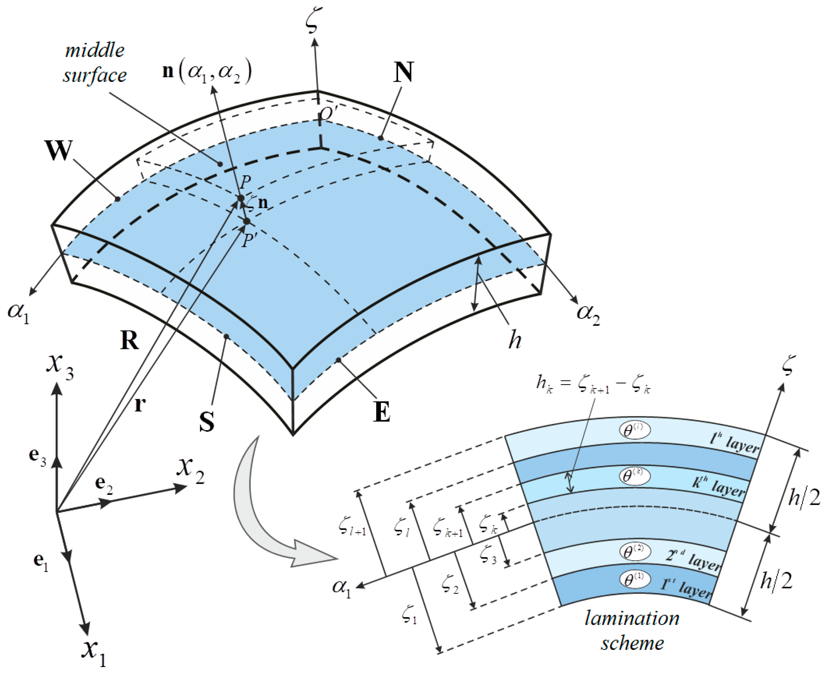
2. Shell Geometry
3. Higher-Order ESL Model
4. Numerical Technique
5. Solution of the Static Problem
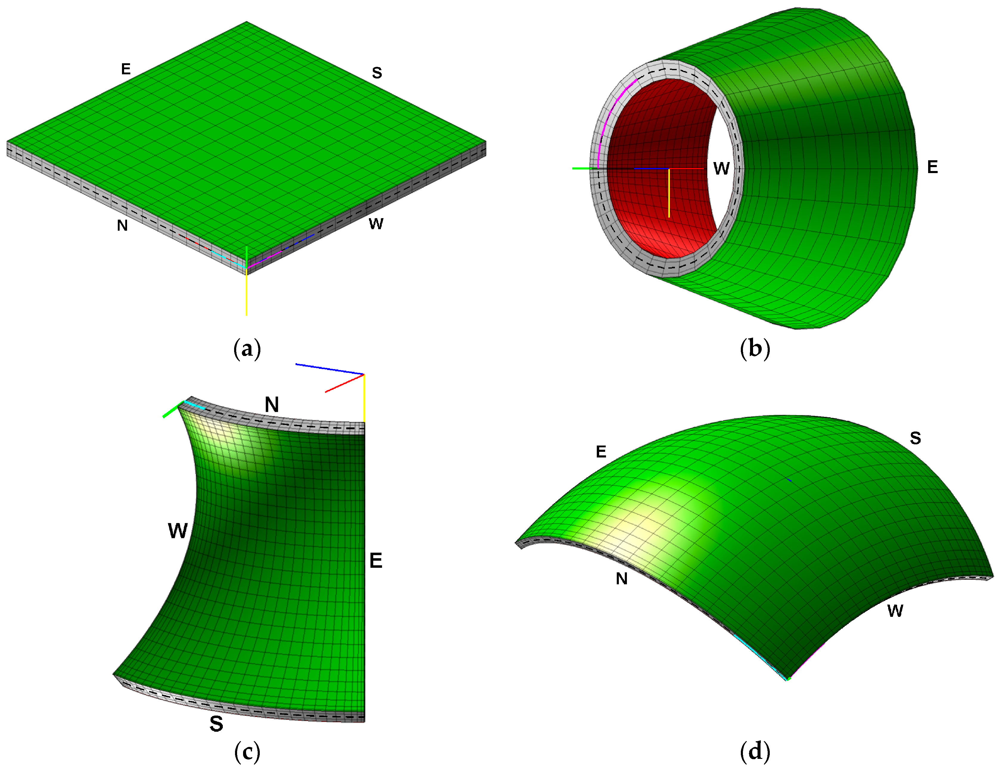
6. Applications
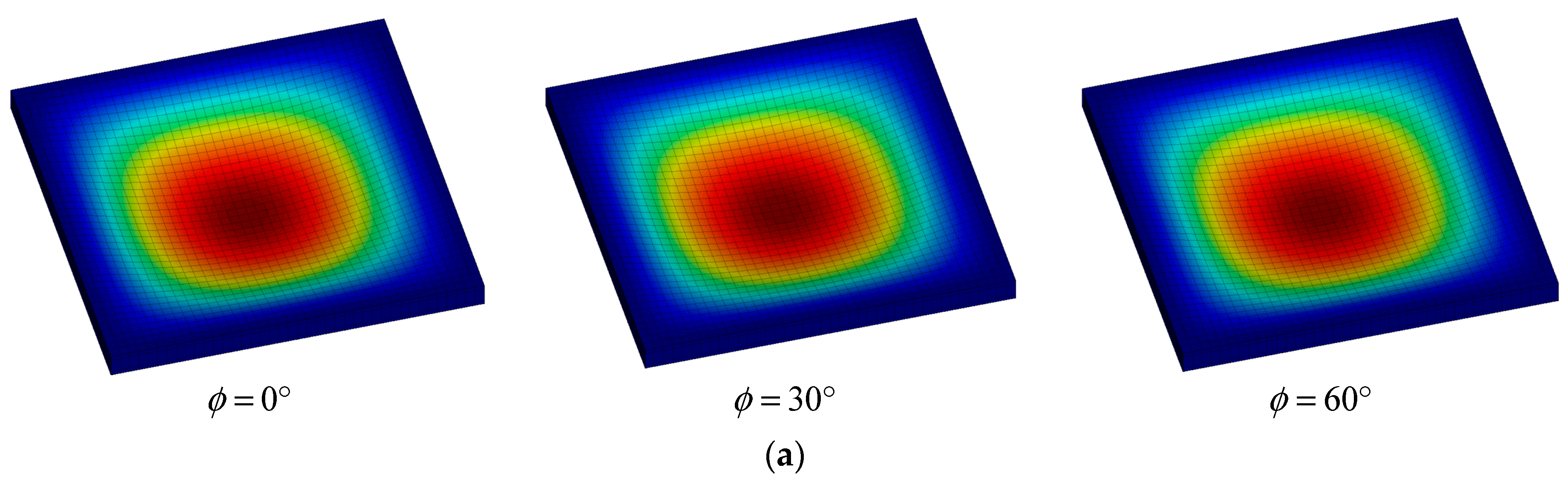
6.1. Square Plate
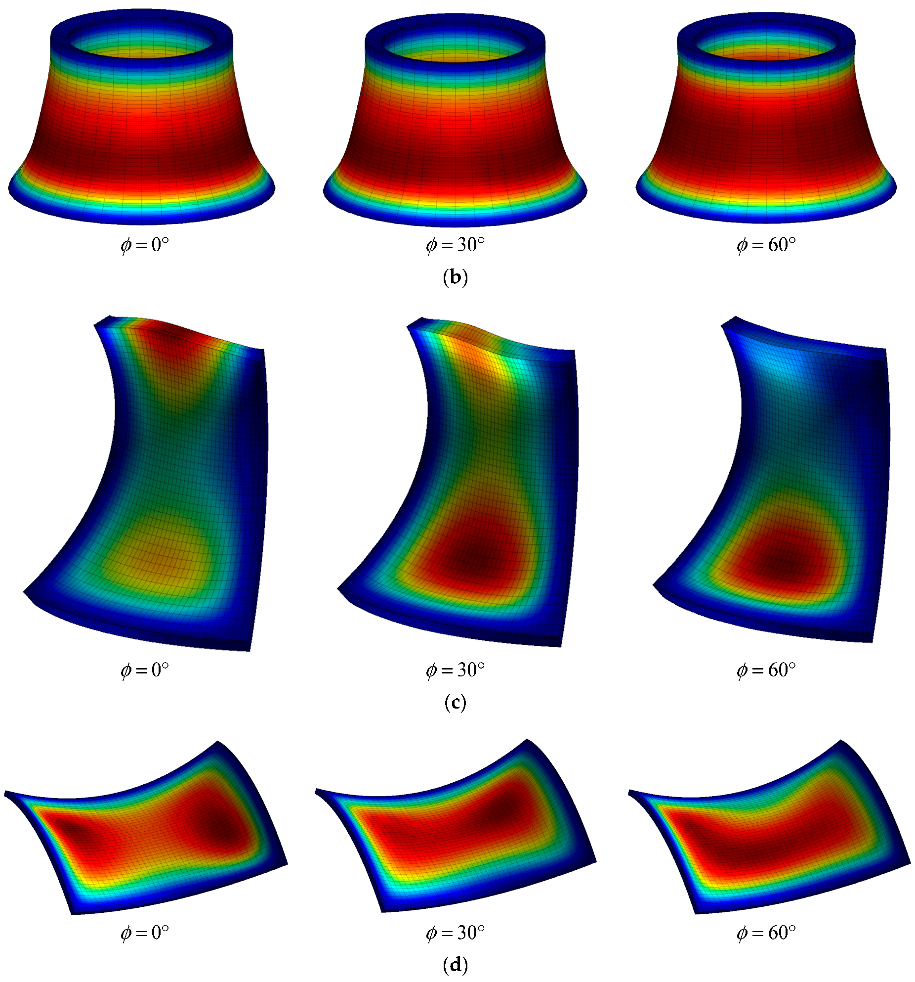
6.2. Conical Shell
6.3. Doubly-Curved Panel of Revolution
6.4. Doubly-Curved Panel of Translation
6.5. Remarks on the Use of the Murakami’s Function
7. Discussion
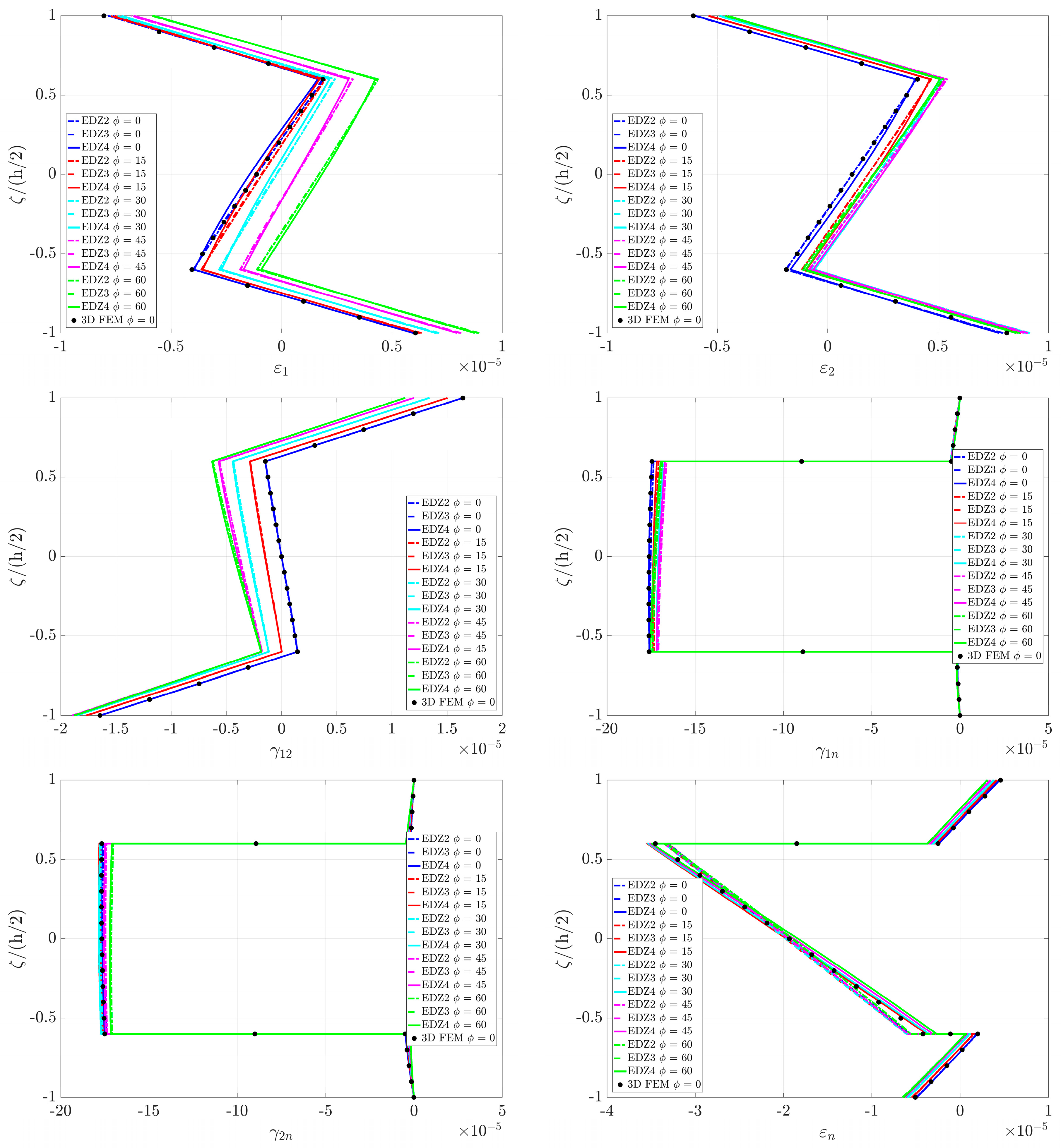
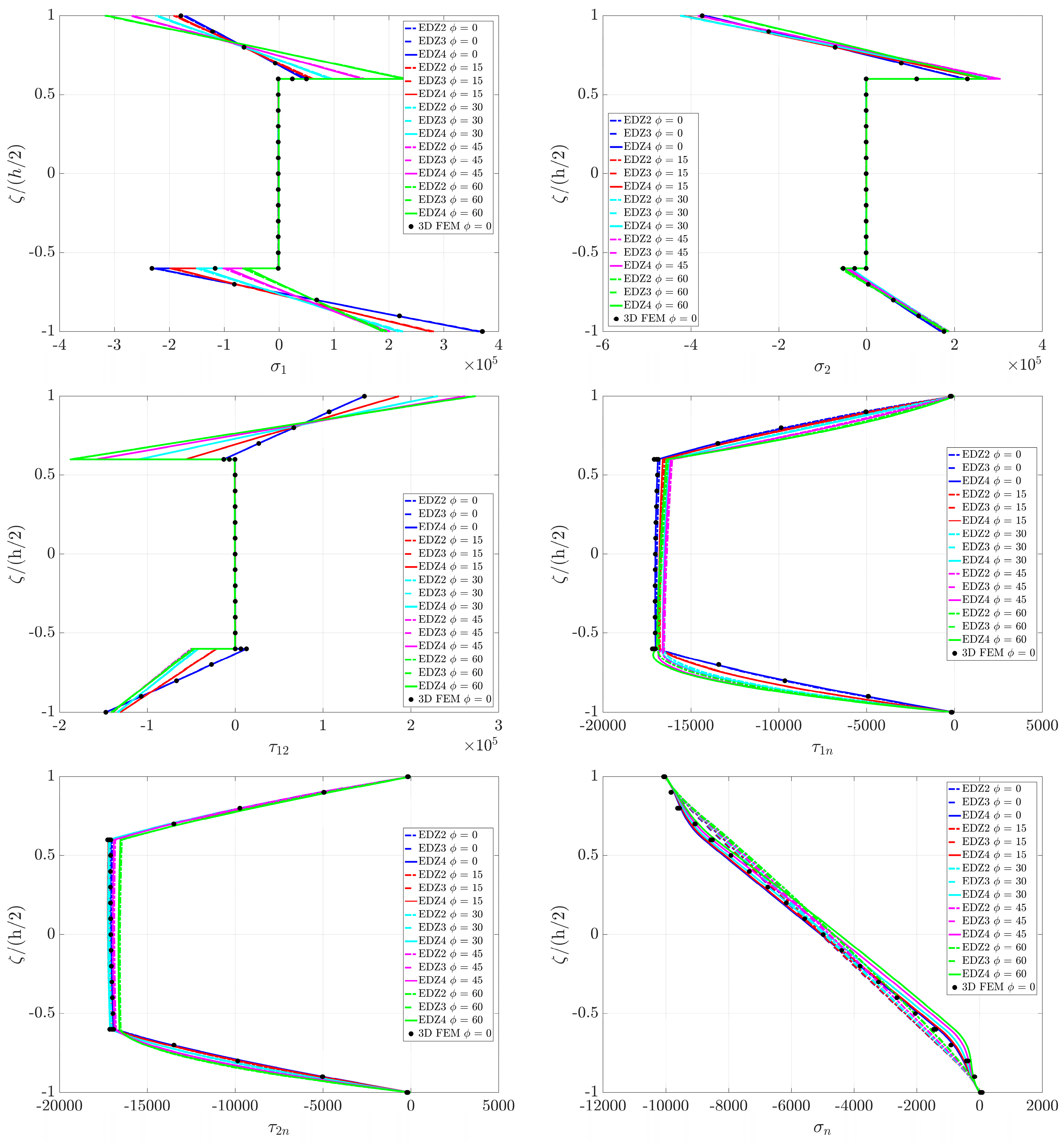
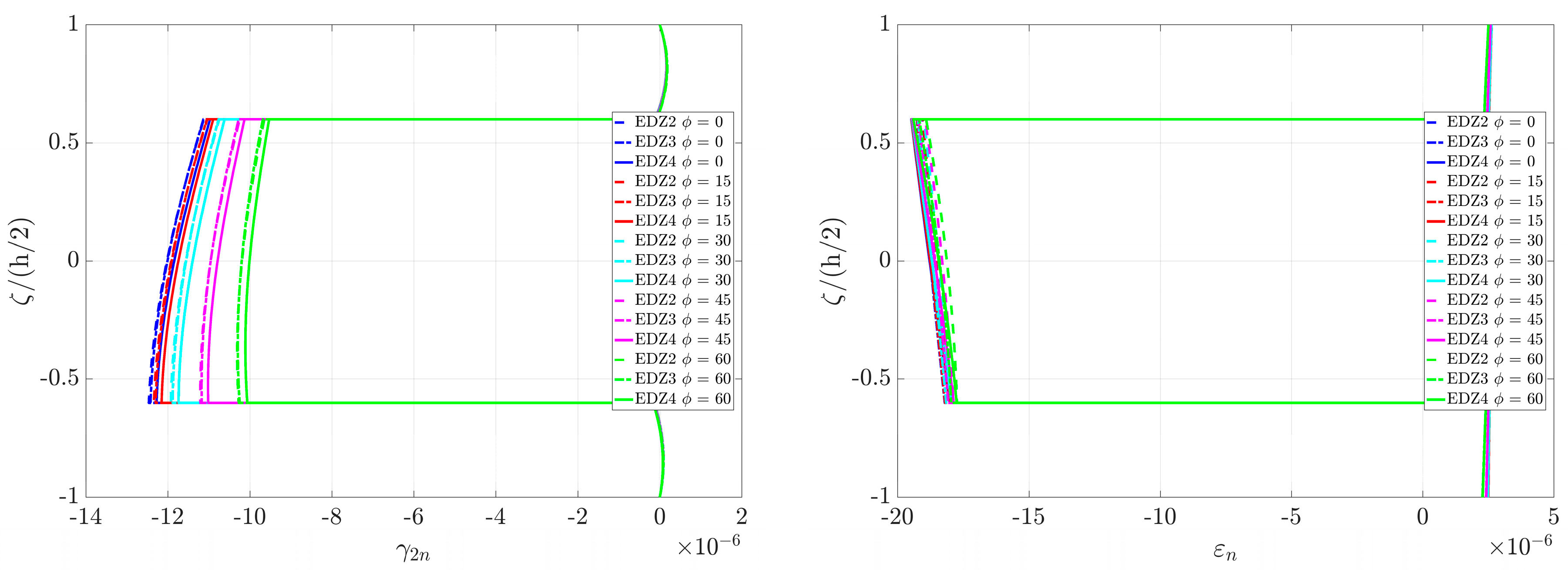
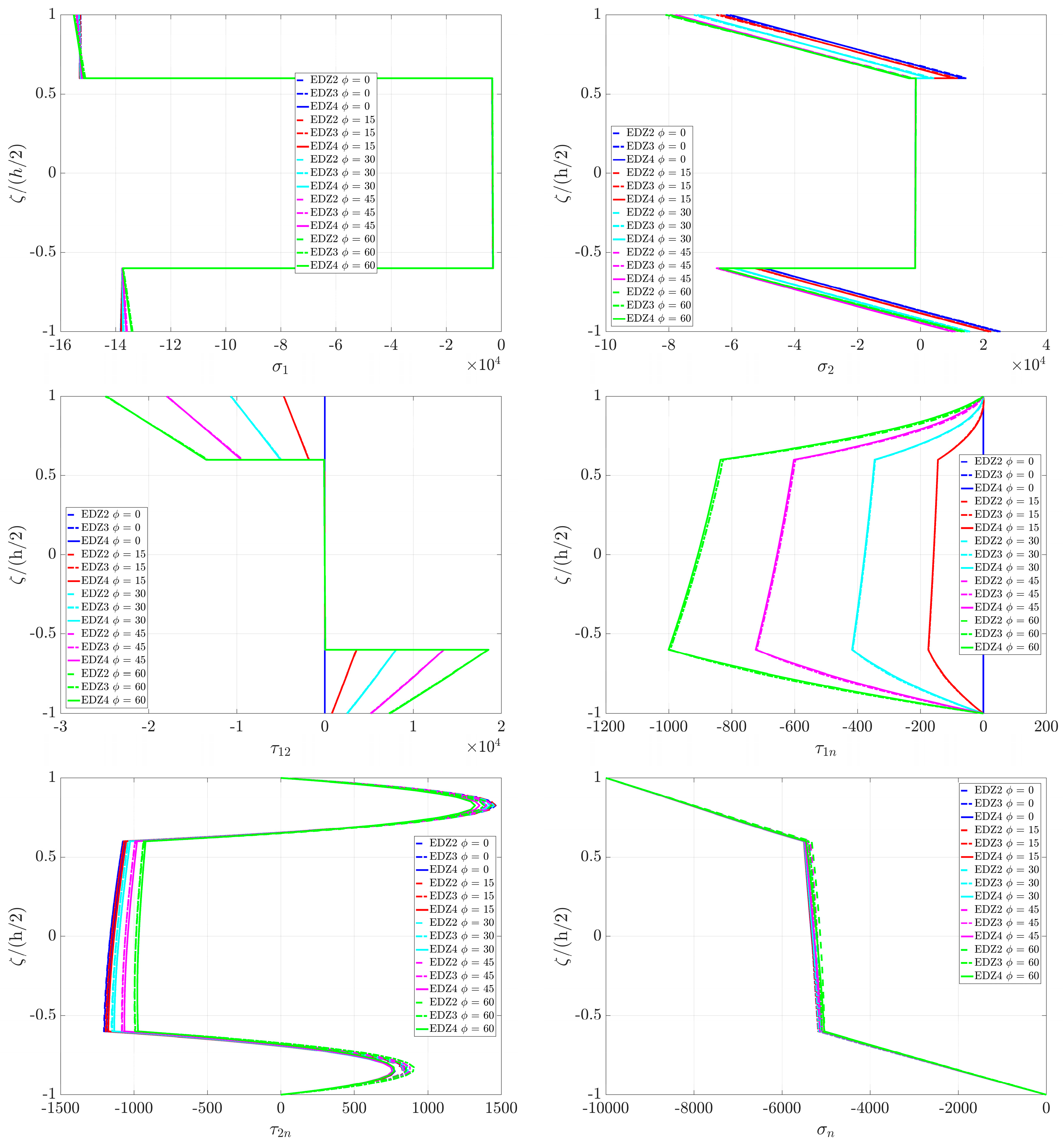
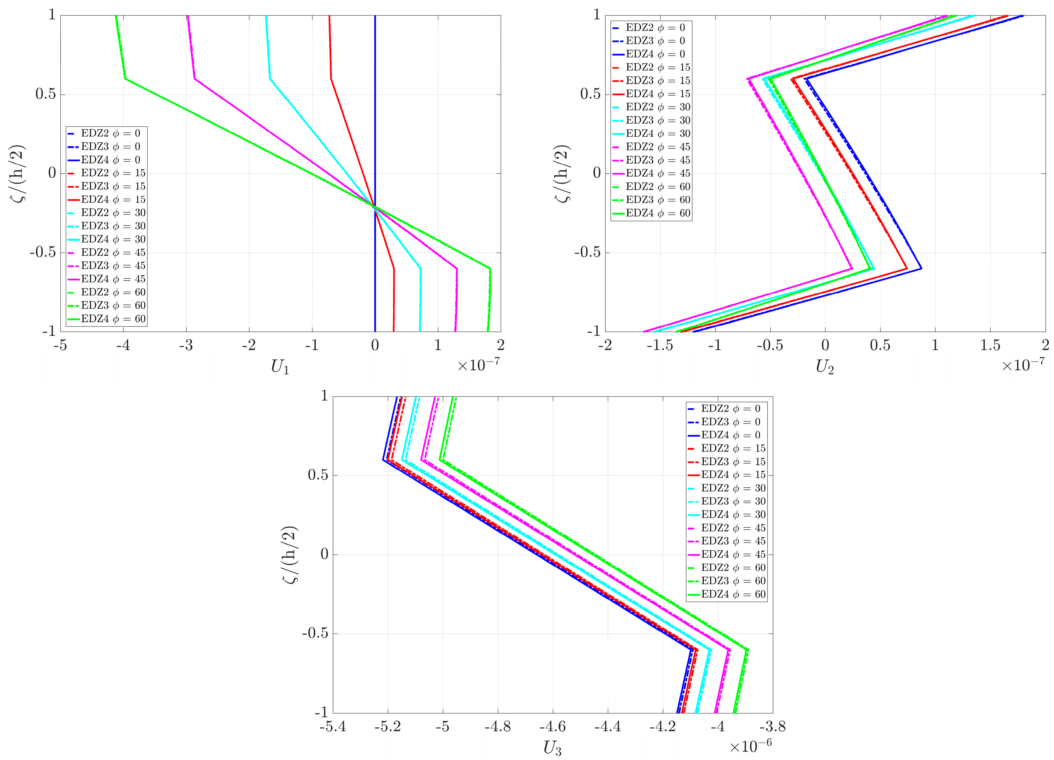
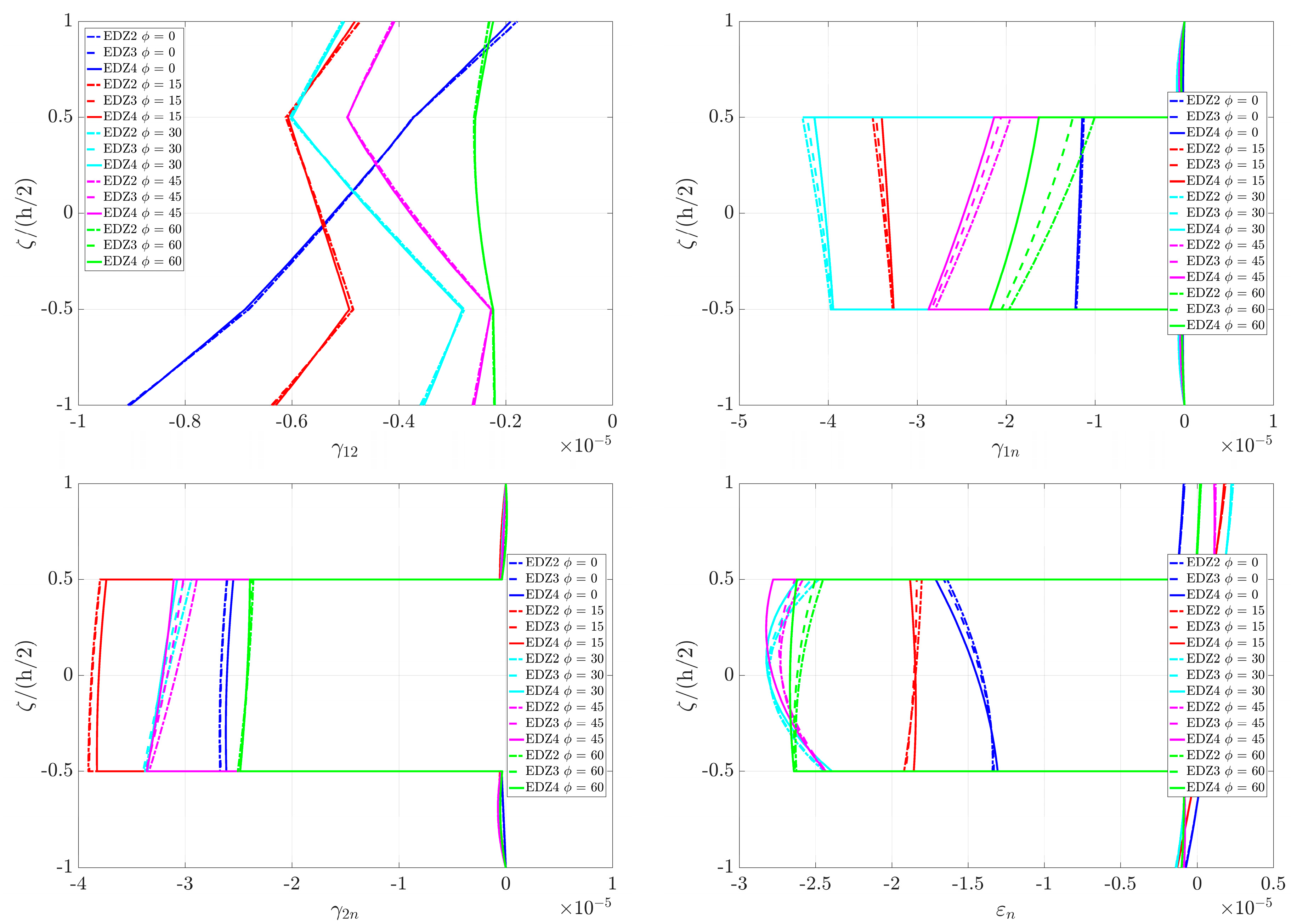
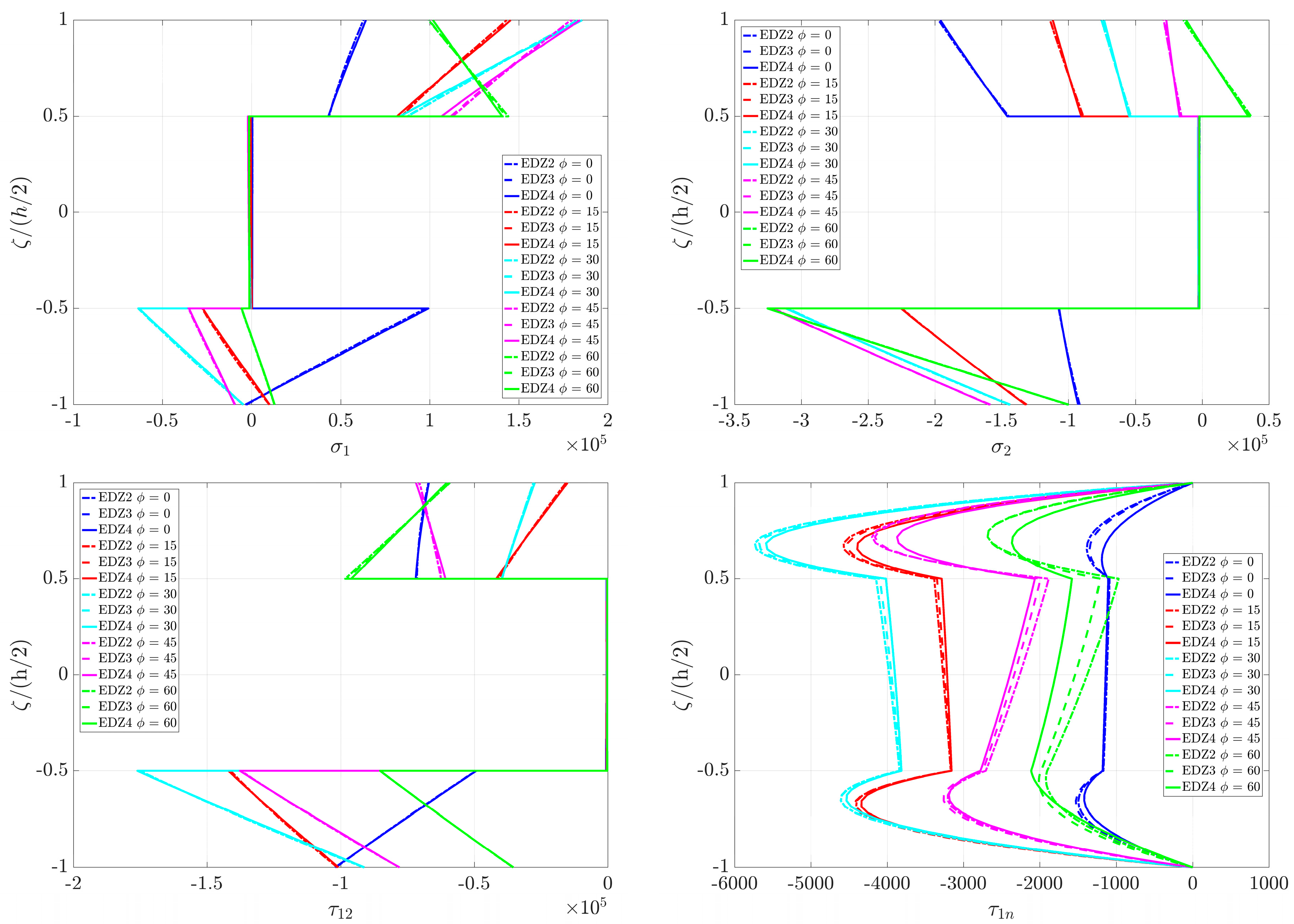
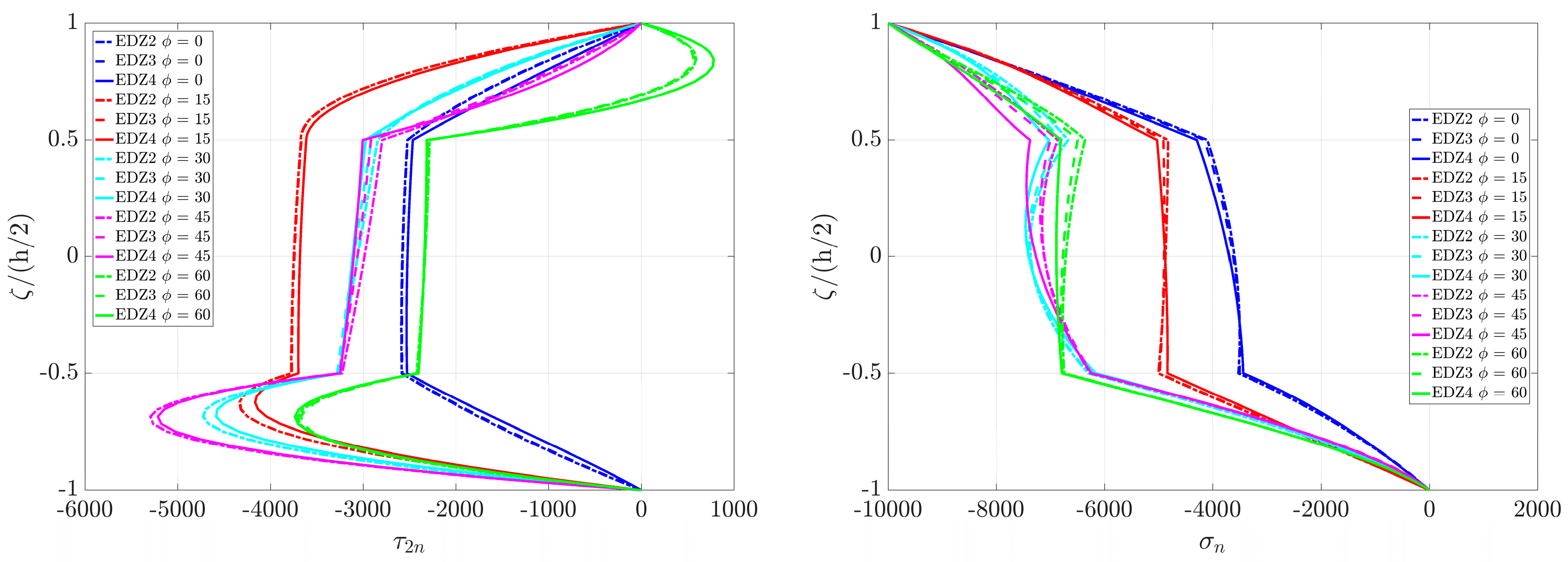
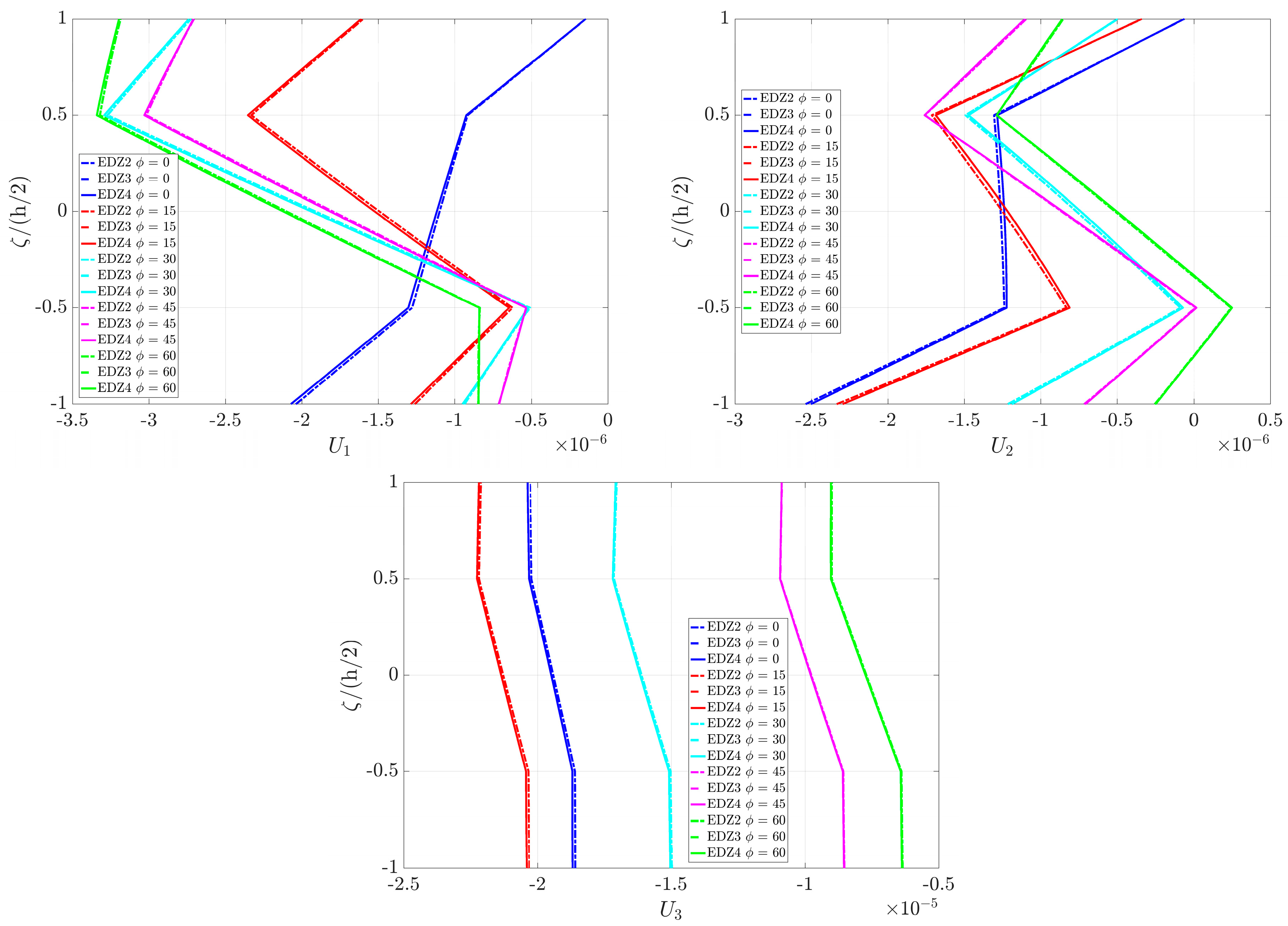
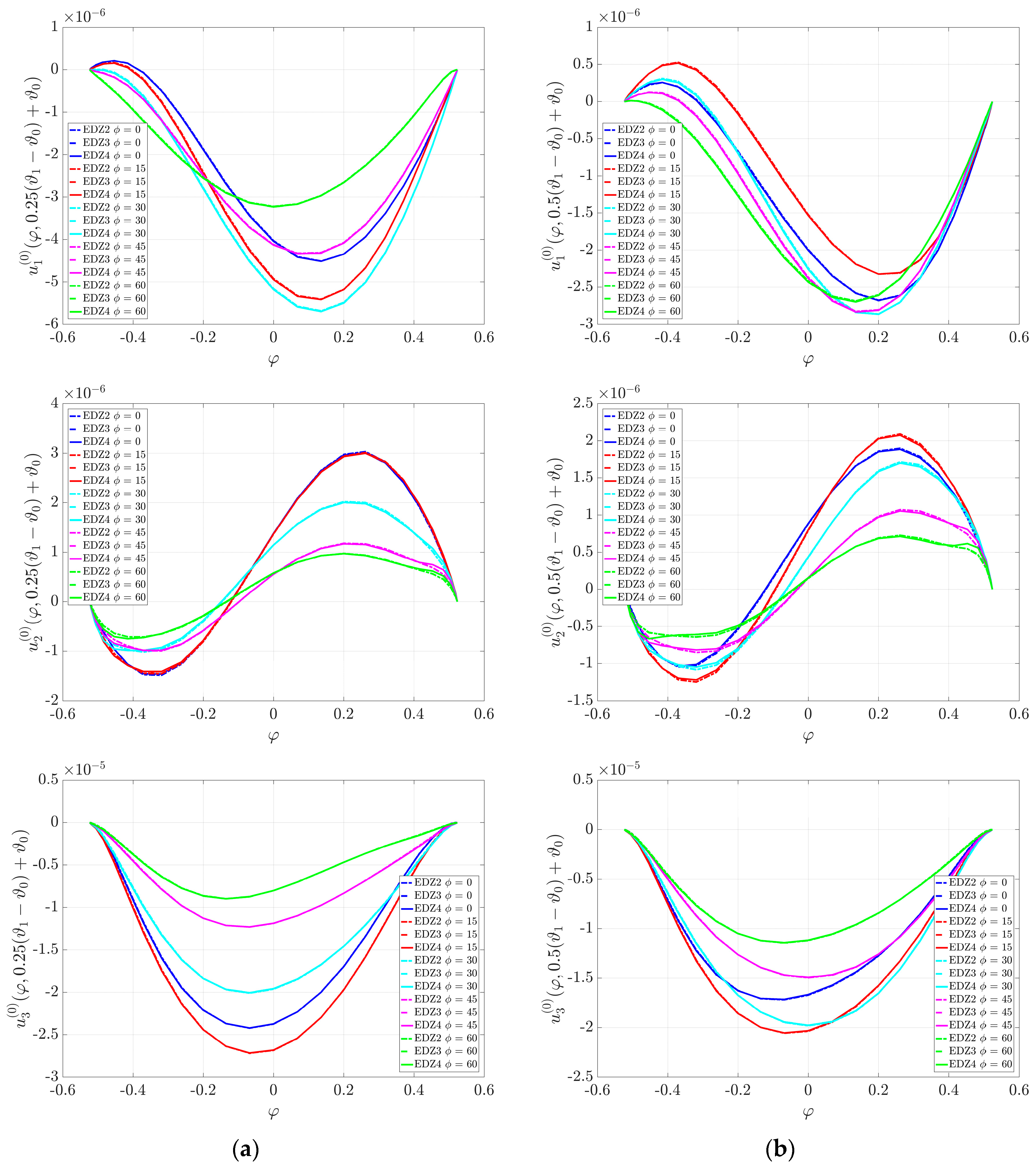
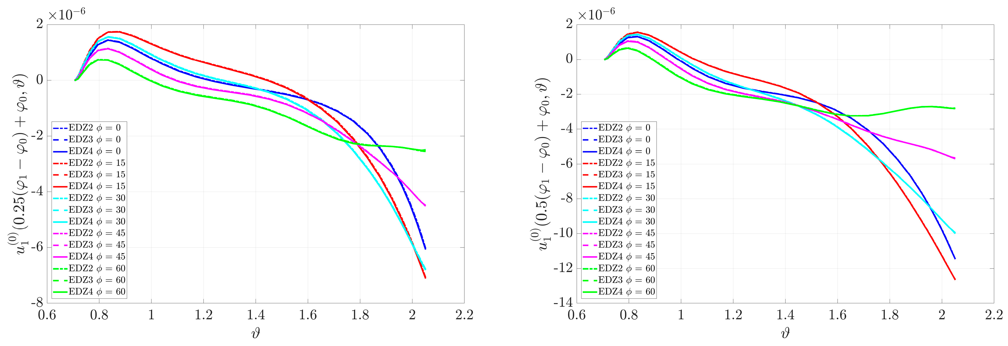
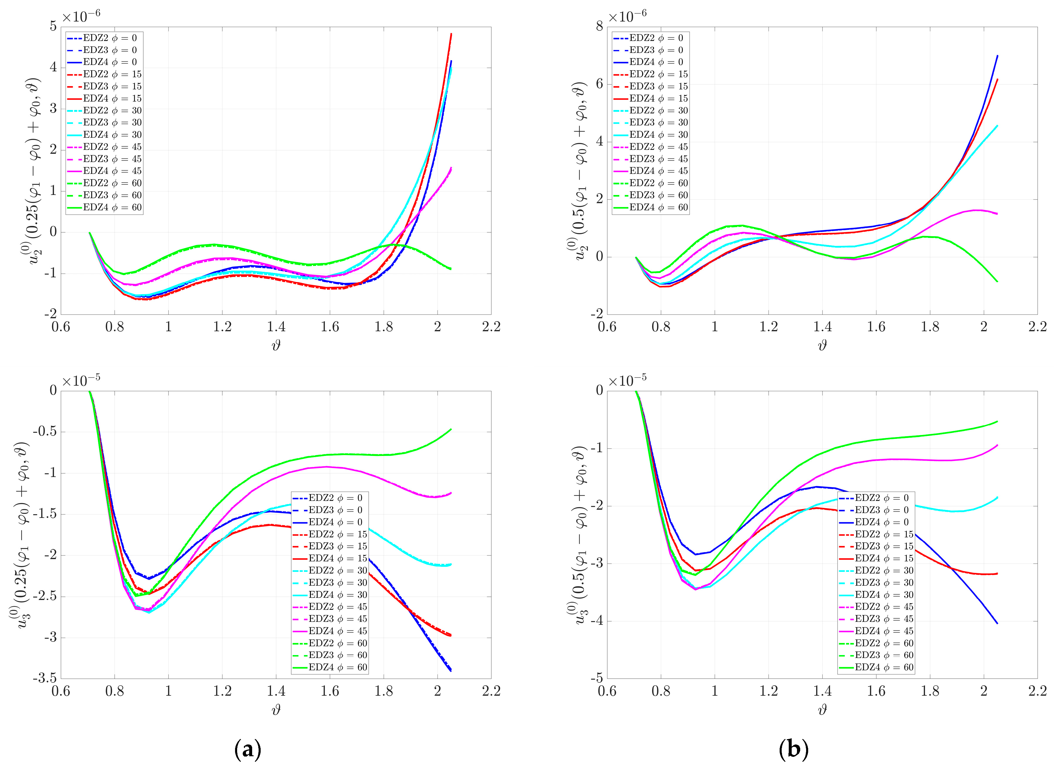
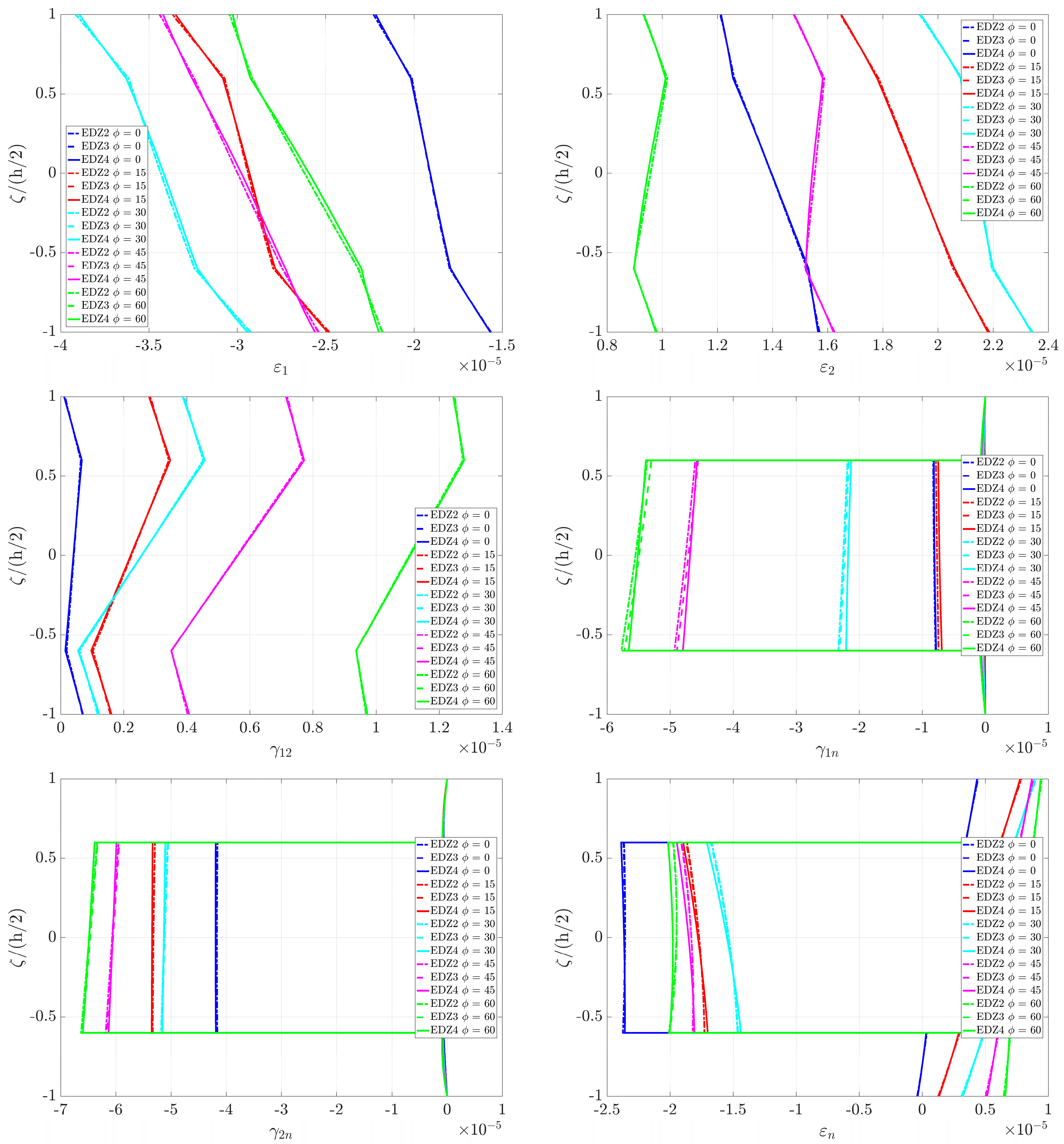
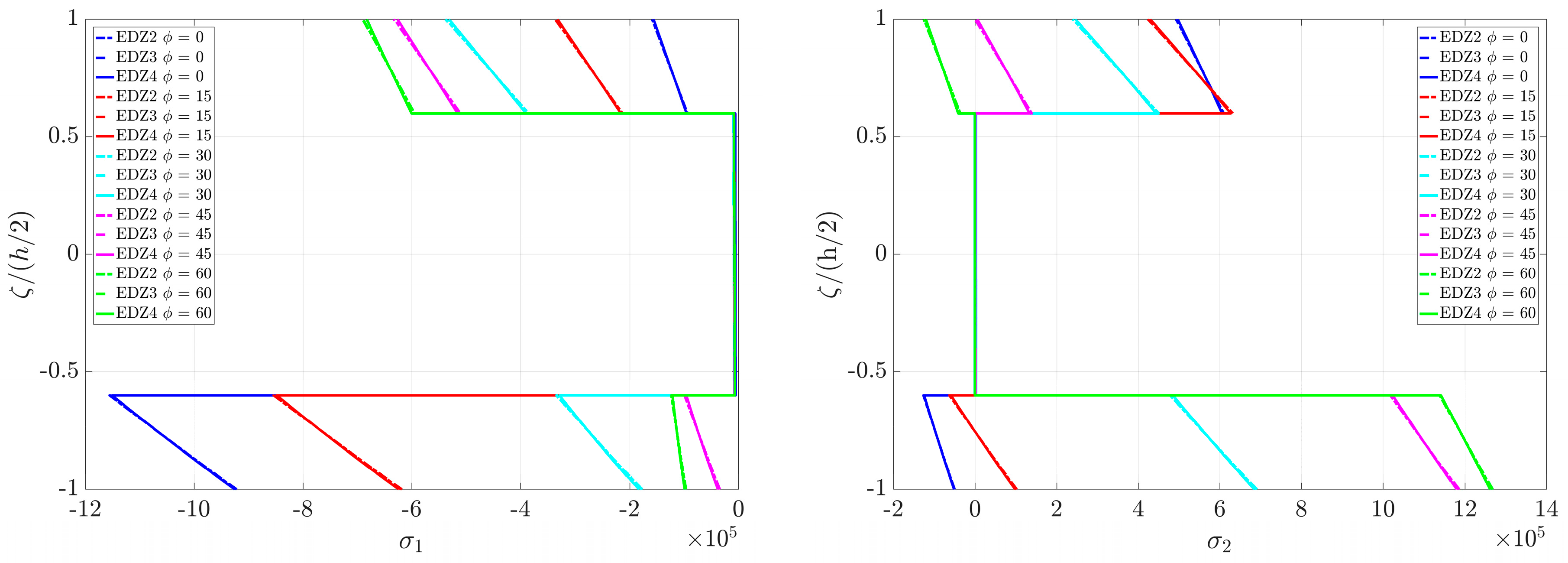
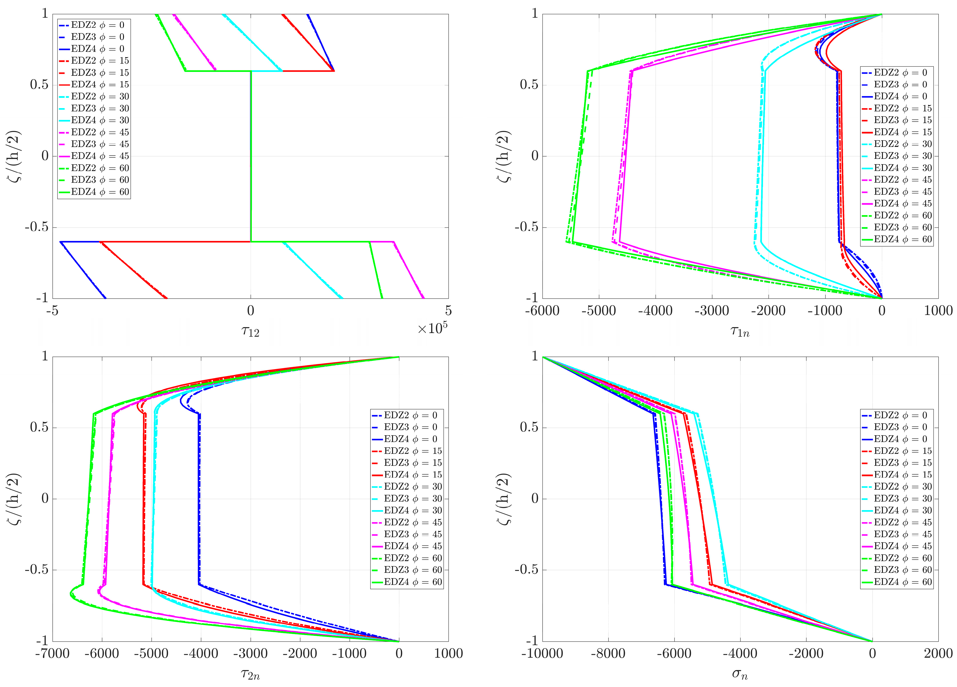
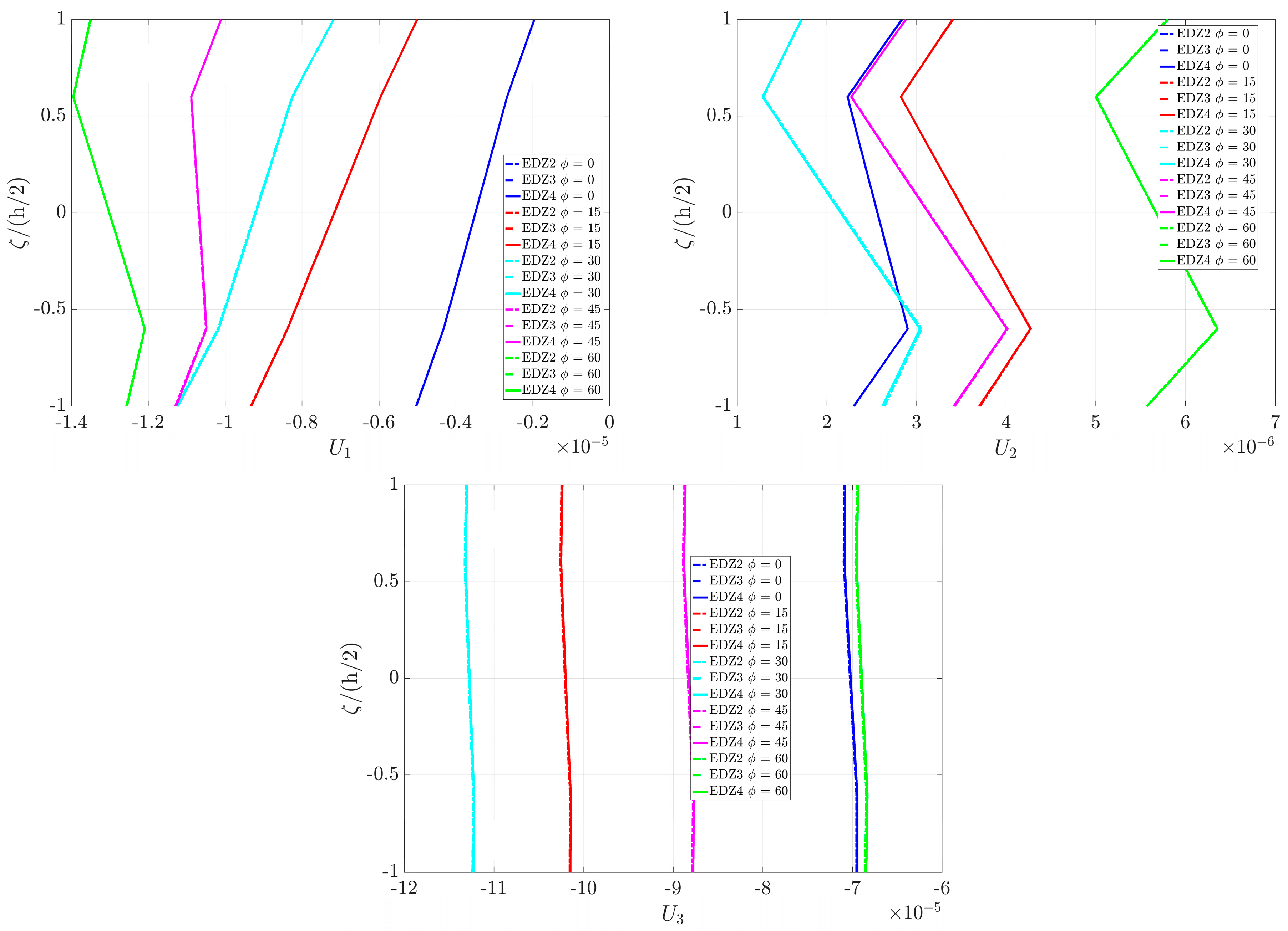
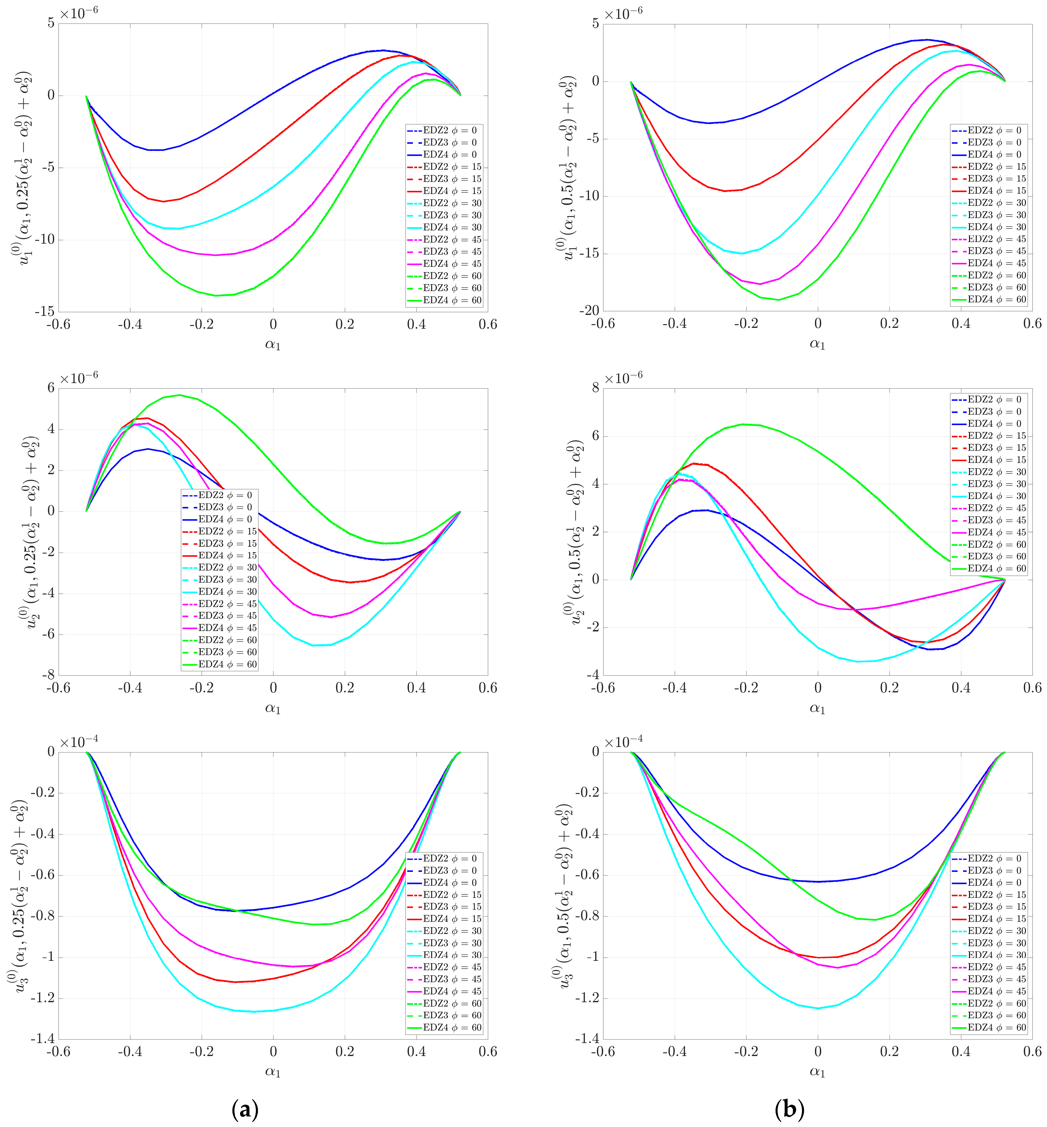
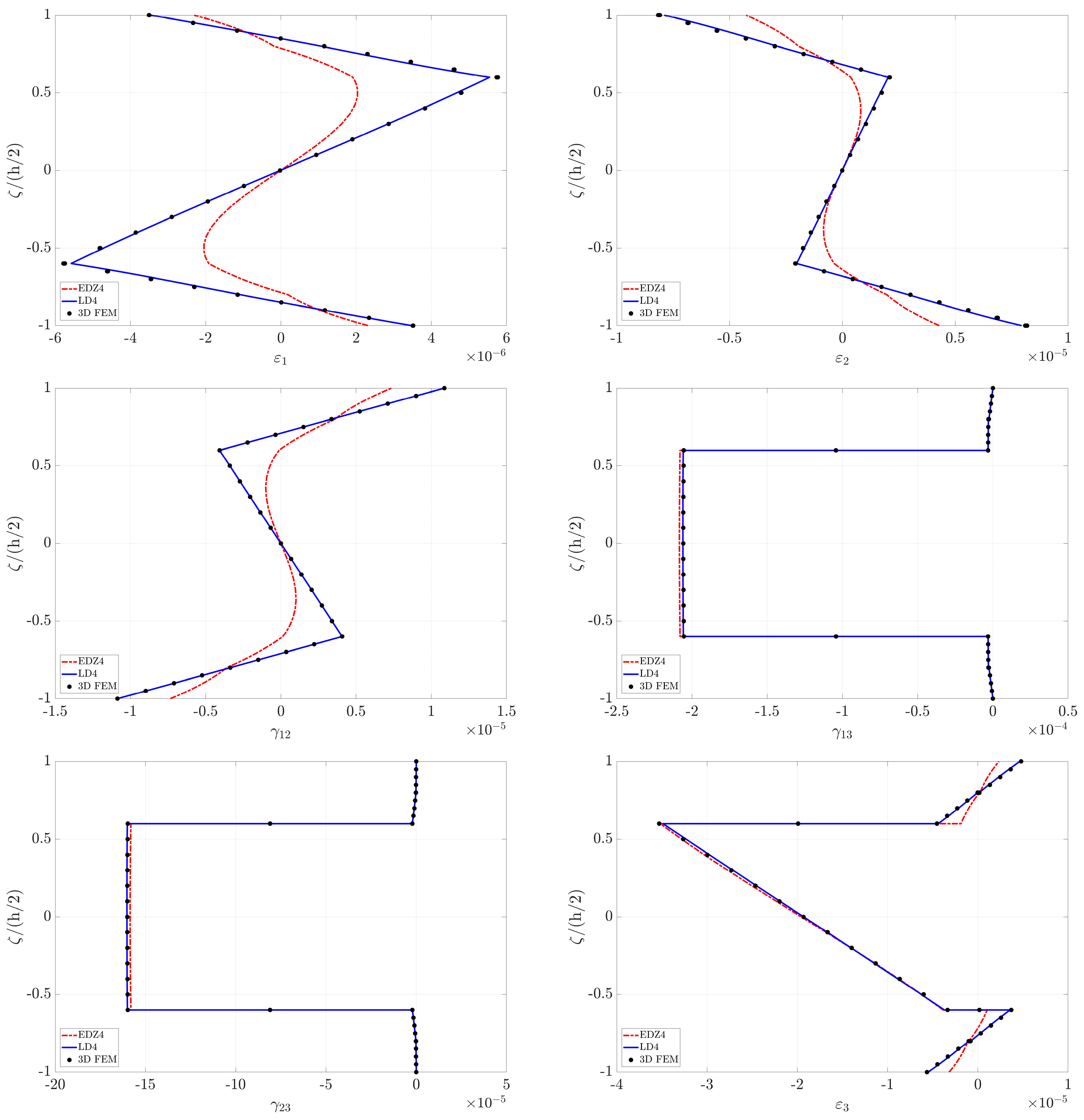
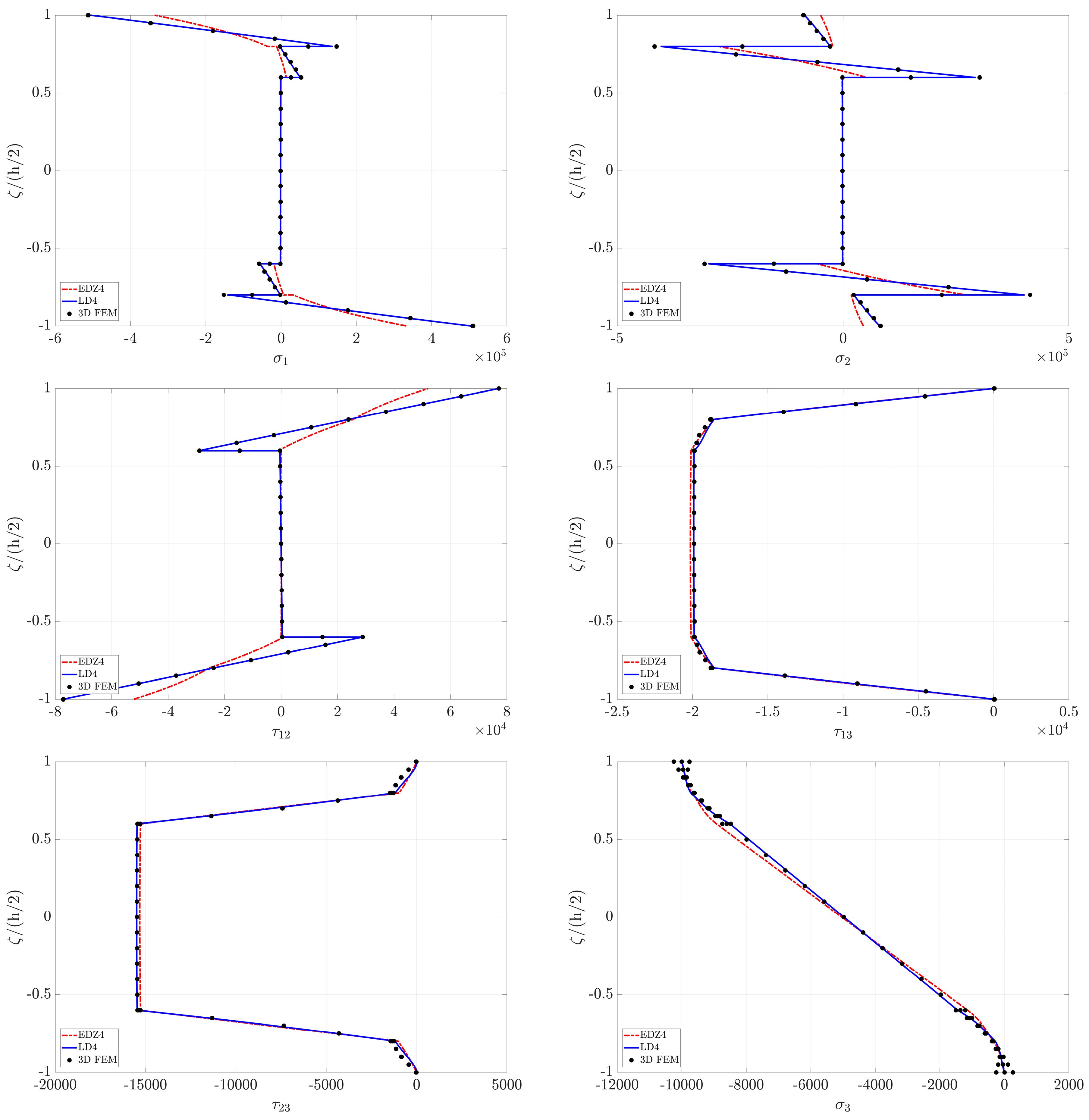
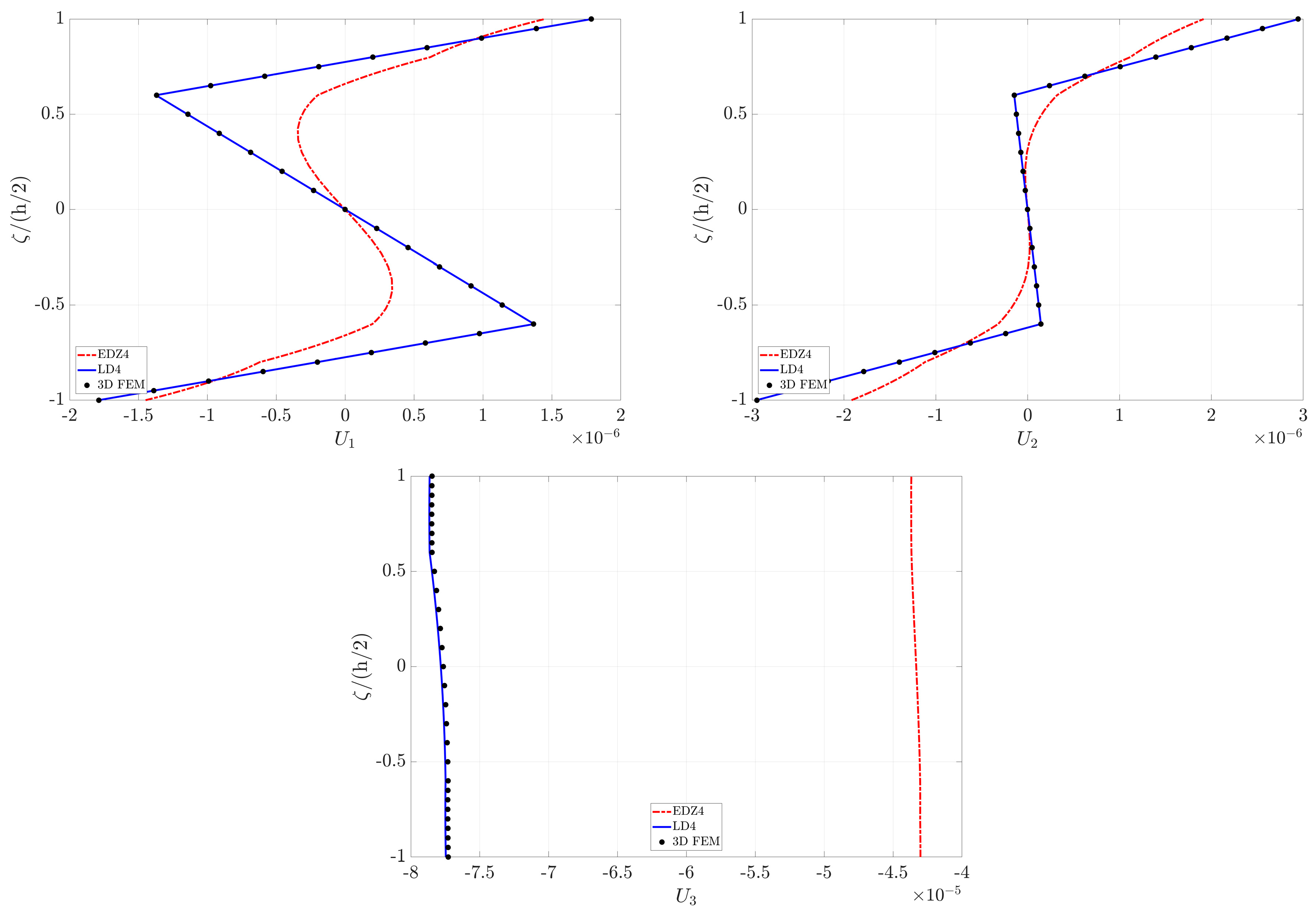
- The soft-core effect is well-captured by means of the Murakami’s function. As highlighted in previous work [56], this function is required to model the so-called zig-zag effect. These aspects are extremely clear in the through-the-thickness profiles of strain, stress and displacement components presented in the paper.
- The higher-order theories employed in this paper provide comparable results. Thus, all these models can be used to deal with similar structural problems. With respect to first-order models, the shear correction factor and the plane stress hypothesis can be neglected, and the mechanical behavior is closer to the three-dimensional one.
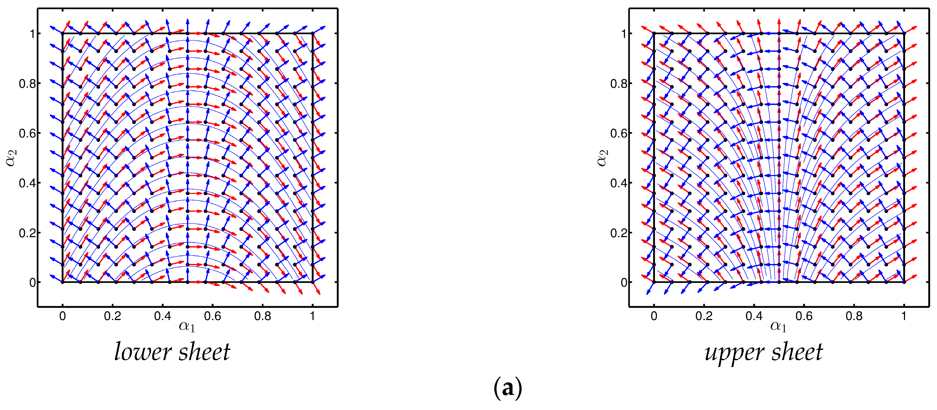
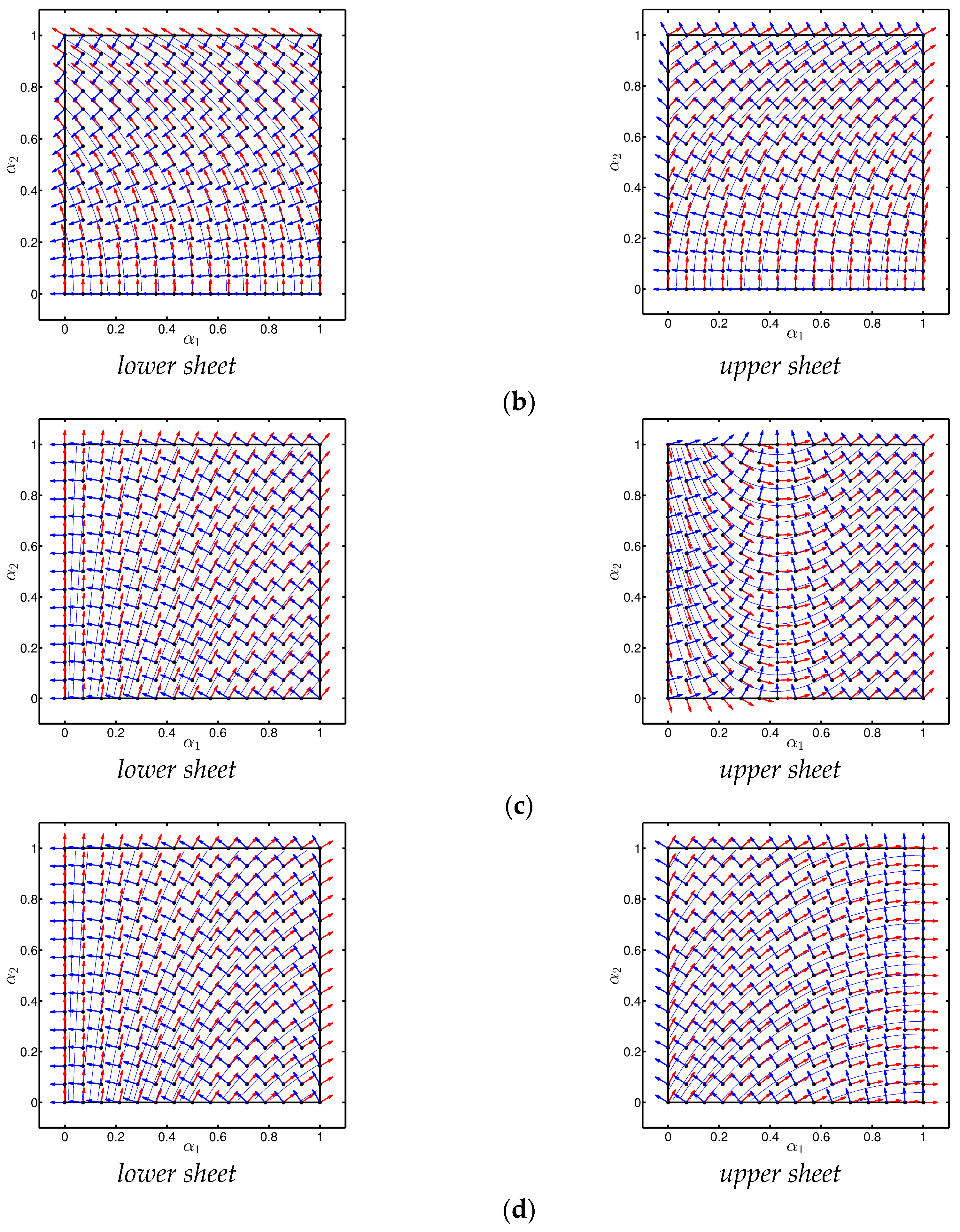
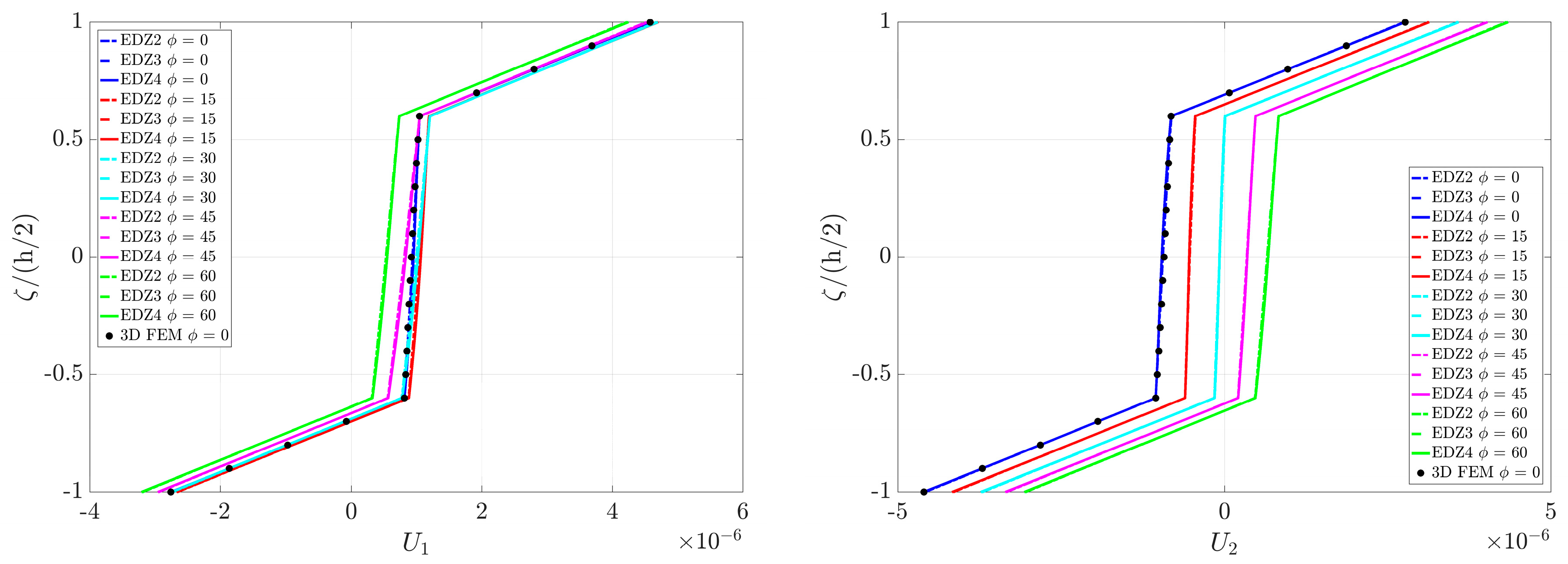
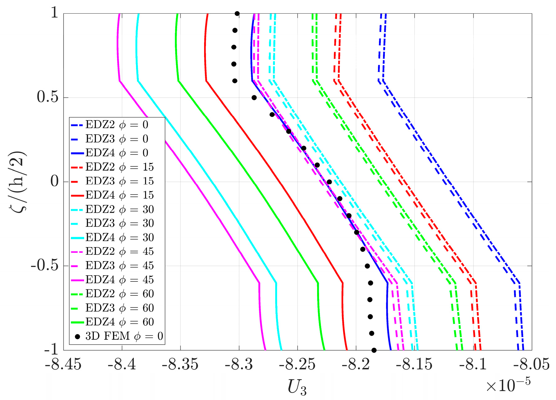
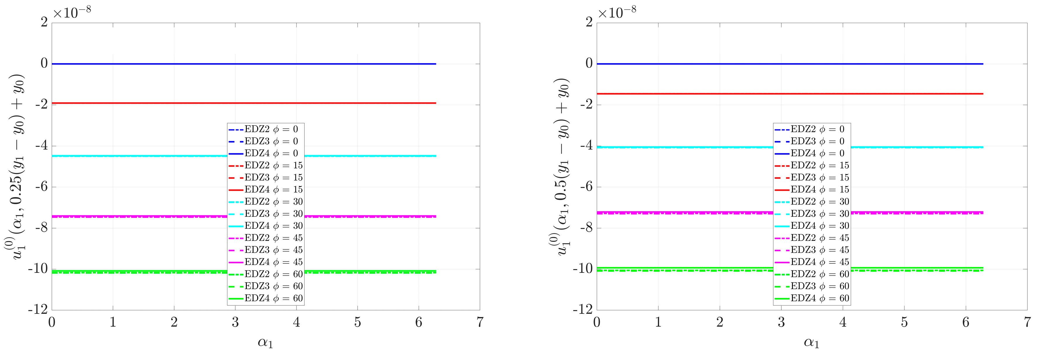
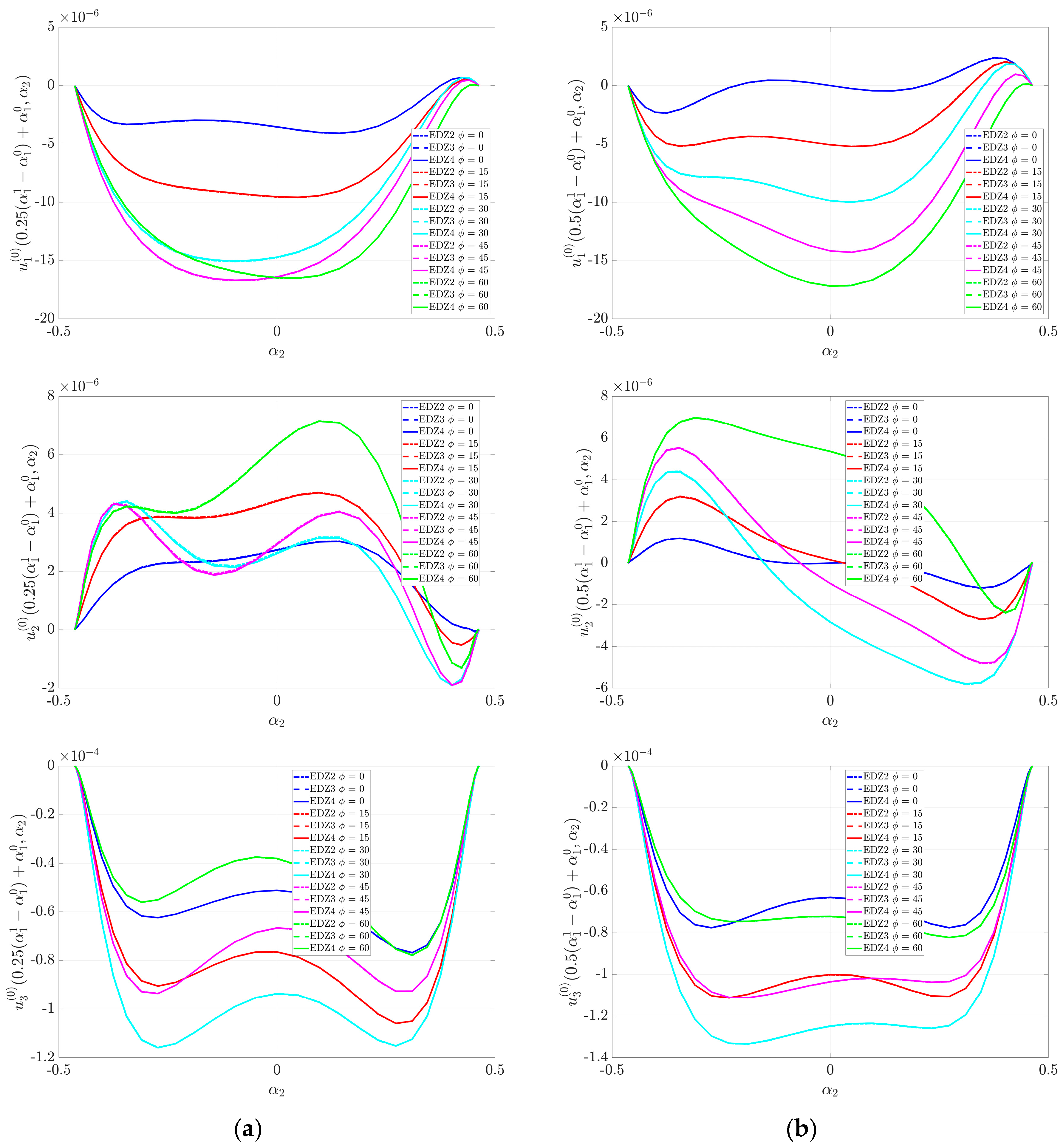
- The linear static behavior is affected by the value of the fiber orientation. Therefore, the angle of the fiber orientation represents a design parameter that can be modified and optimized during the manufacturing process to obtain the desired structural behavior in terms of static response.
- The boundary conditions in terms of generalized displacements on the shell middle surface, as well as stress profiles, are well-enforced. In particular, null displacements are obtained for clamped edges, whereas the normal stress coincides with the value of the corresponding applied load.
- The numerical method employed in the paper represents an accurate tool to deal with similar structural problems.
Acknowledgments
Author Contributions
Conflicts of Interest
References
- Jones, R.M. Mechanics of Composite Materials, 2nd ed.; Taylor & Francis: Philadelphia, PA, USA, 1999. [Google Scholar]
- Vasiliev, V.V.; Morozov, E.V. Mechanics and Analysis of Composite Materials; Elsevier: Oxford, UK, 2001. [Google Scholar]
- Reddy, J.N. Mechanics of Laminated Composite Plates and Shells, 2nd ed.; CRC Press: Boca Raton, FL, USA, 2004. [Google Scholar]
- Tornabene, F.; Fantuzzi, N.; Bacciocchi, M.; Viola, E. Laminated Composite Doubly-Curved Shell Structures. Differential Geometry. Higher-Order Structural Theories; Esculapio: Bologna, Italy, 2016. [Google Scholar]
- Tornabene, F.; Fantuzzi, N.; Bacciocchi, M.; Viola, E. Accurate Inter-Laminar Recovery for Plates and Doubly-Curved Shells with Variable Radii of Curvature Using Layer-Wise Theories. Compos. Struct. 2015, 124, 368–393. [Google Scholar] [CrossRef]
- Fantuzzi, N.; Bacciocchi, M.; Tornabene, F.; Viola, E.; Ferreira, A.J.M. Radial Basis Functions Based on Differential Quadrature Method for the Free Vibration of Laminated Composite Arbitrary Shaped Plates. Compos. Part B Eng. 2015, 78, 65–78. [Google Scholar] [CrossRef]
- Tornabene, F.; Fantuzzi, N.; Bacciocchi, M.; Viola, E. A New Approach for Treating Concentrated Loads in Doubly-Curved Composite Deep Shells with Variable Radii of Curvature. Compos. Struct. 2015, 131, 433–452. [Google Scholar] [CrossRef]
- Tornabene, F.; Fantuzzi, N.; Bacciocchi, M.; Dimitri, R. Dynamic Analysis of Thick and Thin Elliptic Shell Structures Made of Laminated Composite Materials. Compos. Struct. 2015, 133, 278–299. [Google Scholar] [CrossRef]
- Tornabene, F.; Fantuzzi, N.; Bacciocchi, M.; Dimitri, R. Free Vibrations of Composite Oval and Elliptic Cylinders by the Generalized Differential Quadrature Method. Thin Wall. Struct. 2015, 97, 114–129. [Google Scholar] [CrossRef]
- Tornabene, F.; Fantuzzi, N.; Bacciocchi, M. The Local GDQ Method for the Natural Frequencies of Doubly-Curved Shells with Variable Thickness: A General Formulation. Compos. Part B Eng. 2016, 92, 265–289. [Google Scholar] [CrossRef]
- Tornabene, F.; Fantuzzi, N.; Viola, E. Inter-Laminar Stress Recovery Procedure for Doubly-Curved, Singly-Curved, Revolution Shells with Variable Radii of Curvature and Plates Using Generalized Higher-Order Theories and the Local GDQ Method. Mech. Adv. Mater. Struct. 2016, 23, 1019–1045. [Google Scholar] [CrossRef]
- Tornabene, F. General Higher Order Layer-Wise Theory for Free Vibrations of Doubly-Curved Laminated Composite Shells and Panels. Mech. Adv. Mater. Struct. 2016, 23, 1046–1067. [Google Scholar] [CrossRef]
- Fantuzzi, N.; Tornabene, F. Strong Formulation Isogeometric Analysis (SFIGA) for Laminated Composite Arbitrarily Shaped Plates. Compos. Part B Eng. 2016, 96, 173–203. [Google Scholar] [CrossRef]
- Tornabene, F.; Fantuzzi, N.; Bacciocchi, M.; Neves, A.M.A.; Ferreira, A.J.M. MLSDQ Based on RBFs for the Free Vibrations of Laminated Composite Doubly-Curved Shells. Compos. Part B Eng. 2016, 99, 30–47. [Google Scholar] [CrossRef]
- Tornabene, F.; Fantuzzi, N.; Bacciocchi, M. The GDQ Method for the Free Vibration Analysis of Arbitrarily Shaped Laminated Composite Shells Using a NURBS-Based Isogeometric Approach. Compos. Struct. 2016, 154, 190–218. [Google Scholar] [CrossRef]
- Tornabene, F.; Fantuzzi, N.; Bacciocchi, M. On the Mechanics of Laminated Doubly-Curved Shells Subjected to Point and Line Loads. Int. J. Eng. Sci. 2016, 109, 115–164. [Google Scholar] [CrossRef]
- Bacciocchi, M.; Eisenberger, M.; Fantuzzi, N.; Tornabene, F.; Viola, E. Vibration Analysis of Variable Thickness Plates and Shells by the Generalized Differential Quadrature Method. Compos. Struct. 2016, 156, 218–237. [Google Scholar] [CrossRef]
- Tornabene, F.; Fantuzzi, N.; Bacciocchi, M.; Reddy, J.N. An Equivalent Layer-Wise Approach for the Free Vibration Analysis of Thick and Thin Laminated Sandwich Shells. Appl. Sci. 2017, 7, 17. [Google Scholar] [CrossRef]
- Brischetto, S.; Tornabene, F.; Fantuzzi, N.; Bacciocchi, M. Interpretation of Boundary Conditions in the Analytical and Numerical Shell Solutions for Mode Analysis of Multilayered Structures. Int. J. Mech. Sci. 2017, 122, 18–28. [Google Scholar] [CrossRef]
- Tornabene, F.; Fantuzzi, N.; Bacciocchi, M. A New Doubly-Curved Shell Element for the Free Vibrations of Arbitrarily Shaped Laminated Structures Based on Weak Formulation IsoGeometric Analysis. Compos. Struct. 2017, 171, 429–461. [Google Scholar] [CrossRef]
- Tornabene, F.; Fantuzzi, N.; Bacciocchi, M.; Reddy, J.N. A Posteriori Stress and Strain Recovery Procedure for the Static Analysis of Laminated Shells Resting on Nonlinear Elastic Foundation. Compos. Part B Eng. 2017, 126, 162–191. [Google Scholar] [CrossRef]
- Fantuzzi, N.; Tornabene, F.; Bacciocchi, M.; Neves, A.M.A.; Ferreira, A.J.M. Stability and Accuracy of Three Fourier Expansion-Based Strong Form Finite Elements for the Free Vibration Analysis of Laminated Composite Plates. Int. J. Numer. Methods Eng. 2017, 111, 354–382. [Google Scholar] [CrossRef]
- Tornabene, F.; Fantuzzi, N.; Bacciocchi, M. Linear Static Behavior of Damaged Laminated Composite Plates and Shells. Materials 2017, 10, 811. [Google Scholar] [CrossRef] [PubMed]
- Zare Jouneghani, F.; Mohammadi Dashtaki, P.; Dimitri, R.; Bacciocchi, M.; Tornabene, F. First-Order Shear Deformation Theory for Orthotropic Doubly-Curved Shells Based on a Modified Couple Stress Elasticity. Aerosp. Sci. Technol. 2018, 73, 129–147. [Google Scholar] [CrossRef]
- Reddy, J.N.; Chin, C.D. Thermomechanical Analysis of Functionally Graded Cylinders and Plates. J. Therm. Stress. 1998, 21, 593–626. [Google Scholar] [CrossRef]
- Reddy, J.N. Analysis of functionally graded plates. Int. J. Numer. Methods Eng. 2000, 47, 663–684. [Google Scholar] [CrossRef]
- Tornabene, F.; Viola, E. Free Vibration Analysis of Functionally Graded Panels and Shells of Revolution. Meccanica 2009, 44, 255–281. [Google Scholar] [CrossRef]
- Tornabene, F. Free Vibration Analysis of Functionally Graded Conical, Cylindrical Shell and Annular Plate Structures with a Four-parameter Power-Law Distribution. Comput. Methods Appl. Mech. Eng. 2009, 198, 2911–2935. [Google Scholar] [CrossRef]
- Tornabene, F.; Viola, E.; Inman, D.J. 2-D Differential Quadrature Solution for Vibration Analysis of Functionally Graded Conical, Cylindrical Shell and Annular Plate Structures. J. Sound Vib. 2009, 328, 259–290. [Google Scholar] [CrossRef]
- Tornabene, F. 2-D GDQ Solution for Free Vibrations of Anisotropic Doubly-Curved Shells and Panels of Revolution. Compos. Struct. 2011, 93, 1854–1876. [Google Scholar] [CrossRef]
- Reddy, J.N. Microstructure-dependent couple stress theories of functionally graded beams. J. Mech. Phys. Solids 2011, 59, 2382–2399. [Google Scholar] [CrossRef]
- Reddy, J.N.; Kim, J. A nonlinear modified couple stress-based third-order theory of functionally graded plates. Compos. Struct. 2012, 94, 1128–1143. [Google Scholar] [CrossRef]
- Kim, J.; Reddy, J.N. A general third-order theory of functionally graded plates with modified couple stress effect and the von Kármán nonlinearity: Theory and finite element analysis. Acta Mech. 2015, 226, 2973–2998. [Google Scholar] [CrossRef]
- Gutierrez Rivera, M.; Reddy, J.N. Stress analysis of functionally graded shells using a 7-parameter shell element. Mech. Res. Commun. 2016, 78, 60–70. [Google Scholar] [CrossRef]
- Lanc, D.; Turkalj, G.; Vo, T.; Brnic, J. Nonlinear buckling behaviours of thin-walled functionally graded open section beams. Compos. Struct. 2016, 152, 829–839. [Google Scholar] [CrossRef]
- Fazzolari, F.A. Stability Analysis of FGM Sandwich Plates by Using Variable-kinematics Ritz Models. Mech. Adv. Mater. Struct. 2016, 23, 1104–1113. [Google Scholar] [CrossRef]
- Fantuzzi, N.; Tornabene, F.; Viola, E. Four-Parameter Functionally Graded Cracked Plates of Arbitrary Shape: A GDQFEM Solution for Free Vibrations. Mech. Adv. Mater. Struct. 2016, 23, 89–107. [Google Scholar] [CrossRef]
- Fantuzzi, N.; Brischetto, S.; Tornabene, F.; Viola, E. 2D and 3D Shell Models for the Free Vibration Investigation of Functionally Graded Cylindrical and Spherical Panels. Compos. Struct. 2016, 154, 573–590. [Google Scholar] [CrossRef]
- Tornabene, F.; Brischetto, S.; Fantuzzi, N.; Bacciocchi, M. Boundary Conditions in 2D Numerical and 3D Exact Models for Cylindrical Bending Analysis of Functionally Graded Structures. Shock Vib. 2016, 2016, 2373862. [Google Scholar] [CrossRef]
- Tornabene, F.; Fantuzzi, N.; Bacciocchi, M.; Viola, E.; Reddy, J.N. A Numerical Investigation on the Natural Frequencies of FGM Sandwich Shells with Variable Thickness by the Local Generalized Differential Quadrature Method. Appl. Sci. 2017, 7, 131. [Google Scholar] [CrossRef]
- Zare Jouneghani, F.; Dimitri, R.; Bacciocchi, M.; Tornabene, F. Free Vibration Analysis of Functionally Graded Porous Doubly-Curved Shells Based on the First-Order Shear Deformation Theory. Appl. Sci. 2017, 7, 1252. [Google Scholar] [CrossRef]
- Tornabene, F.; Fantuzzi, N.; Bacciocchi, M.; Viola, E. Effect of agglomeration on the natural frequencies of functionally graded carbon nanotube-reinforced laminated composite doubly-curved shells. Compos. Part B Eng. 2016, 89, 187–218. [Google Scholar] [CrossRef]
- Tornabene, F.; Fantuzzi, N.; Bacciocchi, M. Linear Static Response of Nanocomposite Plates and Shells Reinforced by Agglomerated Carbon Nanotubes. Compos. Part B Eng. 2017, 115, 449–476. [Google Scholar] [CrossRef]
- Fantuzzi, N.; Tornabene, F.; Bacciocchi, M.; Dimitri, R. Free vibration analysis of arbitrarily shaped Functionally Graded Carbon Nanotube-reinforced plates. Compos. Part B Eng. 2017, 115, 384–408. [Google Scholar] [CrossRef]
- Banić, D.; Bacciocchi, M.; Tornabene, F.; Ferreira, A.J.M. Influence of Winkler-Pasternak Foundation on the Vibrational Behavior of Plates and Shells Reinforced by Agglomerated Carbon Nanotubes. Appl. Sci. 2017, 7, 1228. [Google Scholar] [CrossRef]
- Tornabene, F.; Bacciocchi, M.; Fantuzzi, N.; Reddy, J.N. Multiscale approach for three-phase CNT/polymer/fiber laminated nanocomposite structures. Polym. Compos. 2017, in press. [Google Scholar] [CrossRef]
- Fraternali, F.; Carpentieri, G.; Amendola, A.; Skelton, R.E.; Nesterenko, V.F. Multiscale tunability of solitary wave dynamics in tensegrity metamaterials. Appl. Phys. Lett. 2014, 105, 201903. [Google Scholar] [CrossRef]
- Fabbrocino, F.; Amendola, A.; Benzoni, G.; Fraternali, F. Seismic application of pentamode lattices. Ing. Sismica-Ital. 2016, 33, 62–70. [Google Scholar]
- Amendola, A.; Smith, C.J.; Goodall, R.; Auricchio, F.; Feo, L.; Benzoni, G.; Fraternali, F. Experimental response of additively manufactured metallic pentamode materials confined between stiffening plates. Compos. Struct. 2016, 142, 254–262. [Google Scholar] [CrossRef]
- Amendola, A.; Carpentieri, G.; Feo, L.; Fraternali, F. Bending dominated response of layered mechanical metamaterials alternating pentamode lattices and confinement plates. Compos. Struct. 2016, 157, 71–77. [Google Scholar] [CrossRef]
- Fraternali, F.; Amendola, A. Mechanical modeling of innovative metamaterials alternating pentamode lattices and confinement plates. J. Mech. Phys. Solids 2017, 99, 259–271. [Google Scholar] [CrossRef]
- Amendola, A.; Benzoni, G.; Fraternali, F. Non-linear elastic response of layered structures, alternating pentamode lattices and confinement plates. Compos. Part B Eng. 2017, 115, 117–123. [Google Scholar] [CrossRef]
- Fabbrocino, F.; Amendola, A. Discrete-to-continuum approaches to the mechanics of pentamode bearings. Compos. Struct. 2017, 167, 219–226. [Google Scholar] [CrossRef]
- Waldhart, C. Design of Tow-Placed, Variable-Stiffness Laminates. Master’s Thesis, Virginia Polytechnic Institute and State University, Blacksburg, VA, USA, 1996. [Google Scholar]
- Blom, A.W. Structural Performance of Fiber-Placed, Variable-Stiffness Composite Conical and Cylindrical Shells. Ph.D. Thesis, Delft University of Technology, Delft, The Netherlands, 2010. [Google Scholar]
- Tornabene, F.; Fantuzzi, N.; Bacciocchi, M. Foam Core Composite Sandwich Plates and Shells with Variable Stiffness: Effect of Curvilinear Fiber Path on the Modal Response. J. Sandw. Struct. Mater. 2017, in press. [Google Scholar] [CrossRef]
- Groh, R.M.J. Non-Classical Effects in Straight-Fibre and Tow-Steered Composite Beams and Plates. Ph.D. Thesis, University of Bristol, Bristol, UK, 2016. [Google Scholar]
- Hyer, M.W.; Charette, R.F. Use of Curvilinear Fiber Format in Composite Structure Design. AIAA J. 1991, 29, 1011–1015. [Google Scholar] [CrossRef]
- Hyer, M.W.; Rust, R.J.; Waters, W.A., Jr. Innovative Design of Composite Structures: Design, Manufacturing, and Testing of Plates Utilizing Curvilinear Fiber Trajectories; NASA-CR-197045; NASA: Washington, WA, USA, 1994.
- Gürdal, Z.; Olmedo, R. In-Plane Response of Laminates with Spatially Varying Fiber Orientations: Variable Stiffness Concept. AIAA J. 1993, 31, 751–758. [Google Scholar] [CrossRef]
- Waldhart, C.; Gürdal, Z.; Ribbens, C. Analysis of tow placed, parallel fiber, variable stiffness laminates. In Proceedings of the 37th AIAA/ASME/ASCE/AHS/ASC Structure, Structural Dynamics and Materials Conference, Salt Lake City, UT, USA, 15–17 April 1996; pp. 2210–2220, AIAA-96-1569-CP. [Google Scholar]
- Setoodeh, S.; Gürdal, Z. Curvilinear fiber design of composite laminae by cellular automata. In Proceedings of the 44th AIAA/ASME/ASCE/AHS/ASC Structures, Structural Dynamics, and Materials Conference, Norfolk, VA, USA, 7–10 April 2003; Volume 7, pp. 5487–5495. [Google Scholar]
- Setoodeh, S.; Gürdal, Z.; Abdalla, M.M.; Watson, L.T. Design of variable stiffness composite laminates for maximum bending stiffness. In Proceedings of the 10th AIAA/ISSMO Multidisciplinary Analysis and Optimization Conference, Albany, NY, USA, 30 August–1 September 2004; Volume 4, pp. 2505–2512. [Google Scholar]
- Setoodeh, S.; Gürdal, Z.; Watson, L.T. Design of variable-stiffness composite layers using cellular automata. Comput. Methods Appl. Mech. Eng. 2006, 195, 836–851. [Google Scholar] [CrossRef]
- Jegley, D.C.; Tatting, B.F.; Gürdal, Z. Optimization of elastically tailored tow-placed plates with holes. In Proceedings of the 44th AIAA/ASME/ASCE/AHS/ASC Structures, Structural Dynamics, and Materials Conference, Norfolk, VA, USA, 7–10 April 2003. [Google Scholar]
- Abdalla, M.M.; Setoodeh, S.; Gürdal, Z. Design of variable stiffness composite panels for maximum fundamental frequency using lamination parameters. Compos. Struct. 2007, 81, 283–291. [Google Scholar] [CrossRef]
- Lopes, C.S.; Camanho, P.P.; Gürdal, Z.; Tatting, B.F. Progressive failure analysis of tow-placed variable-stiffness composite panels. Int. J. Solids Struct. 2007, 44, 8493–8516. [Google Scholar] [CrossRef]
- Gürdal, Z.; Tatting, B.F.; Wu, C.K. Variable stiffness composite panels: Effects of stiffness variation on the in-plane and buckling response. Compos. Part A Appl. Sci. Manuf. 2008, 39, 911–922. [Google Scholar] [CrossRef]
- Blom, A.W.; Setoodeh, S.; Hol, J.M.A.M.; Gürdal, Z. Design of variable-stiffness conical shells for maximum fundamental eigenfrequency. Comput. Struct. 2008, 86, 870–878. [Google Scholar] [CrossRef]
- Blom, A.W.; Tatting, B.F.; Hol, J.M.A.M.; Gürdal, Z. Fiber path definitions for elastically tailored conical shells. Compos. Part B Eng. 2009, 40, 77–84. [Google Scholar] [CrossRef]
- Blom, A.W.; Stickler, P.B.; Gürdal, Z. Optimization of a composite cylinder under bending by tailoring stiffness properties in circumferential direction. Compos. Part B Eng. 2010, 41, 157–165. [Google Scholar] [CrossRef]
- Akhavan, H.; Ribeiro, P. Natural modes of vibration of variable stiffness composite laminates with curvilinear fibers. Compos. Struct. 2011, 93, 3040–3047. [Google Scholar] [CrossRef]
- Honda, S.; Narita, Y. Natural frequencies and vibration modes of laminated composite plates reinforced with arbitrary curvilinear fiber shape paths. J. Sound Vib. 2012, 311, 180–191. [Google Scholar] [CrossRef]
- Díaz, J.; Fagiano, C.; Abdalla, M.M.; Gürdal, Z.; Hernández, S. A study of interlaminar stresses in variable stiffness plates. Compos. Struct. 2012, 94, 1192–1199. [Google Scholar] [CrossRef]
- Coburn, B.H.; Wu, Z.; Weaver, P.M. Buckling analysis of stiffened variable angle tow panels. Compos. Struct. 2014, 111, 259–270. [Google Scholar] [CrossRef]
- Raju, G.; Wu, Z.; Weaver, P.M. Buckling and postbuckling of variable angle tow composite plates under in-plane shear loading. Int. J. Solids Struct. 2015, 58, 270–287. [Google Scholar] [CrossRef]
- White, S.C.; Weaver, P.M.; Wu, K.C. Post-buckling analyses of variable-stiffness composite cylinders in axial compression. Compos. Struct. 2015, 123, 190–203. [Google Scholar] [CrossRef]
- Yazdani, S.; Ribeiro, P. A layerwise p-version finite element formulation for free vibration analysis of thick composite laminates with curvilinear fibres. Compos. Struct. 2015, 120, 531–542. [Google Scholar] [CrossRef]
- Ribeiro, P.; Stoykov, S. Forced periodic vibrations of cylindrical shells in laminated composites with curvilinear fibres. Compos. Struct. 2015, 131, 462–478. [Google Scholar] [CrossRef]
- Ribeiro, P. Non-linear modes of vibration of thin cylindrical shells in composite laminates with curvilinear fibres. Compos. Struct. 2015, 122, 184–197. [Google Scholar] [CrossRef]
- Ribeiro, P. Linear modes of vibration of cylindrical shells in composite laminates reinforced by curvilinear fibres. J. Vib. Control 2016, 22, 4141–4158. [Google Scholar] [CrossRef]
- Akhavan, H.; Ribeiro, P. Geometrically non-linear periodic forced vibrations of imperfect laminates with curved fibres by the shooting method. Compos. Part B Eng. 2017, 109, 286–296. [Google Scholar] [CrossRef]
- Vescovini, R.; Dozio, L. A variable-kinematic model for variable stiffness plates: Vibration and buckling analysis. Compos. Struct. 2016, 142, 15–26. [Google Scholar] [CrossRef]
- Groh, R.M.J.; Weaver, P.M. A computationally efficient 2D model for inherently equilibrated 3D stress predictions in heterogeneous laminated plates. Part II: Model validation. Compos. Struct. 2016, 156, 186–217. [Google Scholar] [CrossRef]
- Madeo, A.; Groh, R.M.J.; Zucco, G.; Weaver, P.M.; Zagari, G.; Zinno, R. Post-buckling analysis of variable-angle tow composite plates using Koiter’s approach and the finite element method. Thin Wall. Struct. 2017, 110, 1–13. [Google Scholar] [CrossRef]
- Khani, A.; Abdalla, M.M.; Gürdal, Z.; Sinke, J.; Buitenhuis, A.; Van Tooren, M.J.L. Design, manufacturing and testing of a fibre steered panel with a large cut-out. Compos. Struct. 2017, 180, 821–830. [Google Scholar] [CrossRef]
- Demasi, L.; Biagini, G.; Vannucci, F.; Santarpia, E.; Cavallaro, R. Equivalent Single Layer, Zig-Zag, and Layer Wise theories for variable angle tow composites based on the Generalized Unified Formulation. Compos. Struct. 2017, 177, 54–79. [Google Scholar] [CrossRef]
- Oliveri, V.; Milazzo, A.; Weaver, P.M. Thermo-mechanical post-buckling analysis of variable angle tow composite plate assemblies. Compos. Struct. 2018, 183, 620–635. [Google Scholar] [CrossRef]
- Tornabene, F.; Fantuzzi, N.; Bacciocchi, M.; Viola, E. Higher-order theories for the free vibrations of doubly-curved laminated panels with curvilinear reinforcing fibers by means of a local version of the GDQ method. Compos. Part B Eng. 2015, 81, 196–230. [Google Scholar] [CrossRef]
- Tornabene, F.; Fantuzzi, N.; Bacciocchi, M. Higher-order structural theories for the static analysis of doubly-curved laminated composite panels reinforced by curvilinear fibers. Thin Wall. Struct. 2016, 102, 222–245. [Google Scholar] [CrossRef]
- Blom, A.W.; Lopes, C.S.; Keomwijk, P.J.; Gürdal, Z.; Camanho, P.P. A theoretical model to study the influence of tow-drop areas on the stiffness and strength of variable-stiffness laminates. J. Compos. Mater. 2009, 43, 403–425. [Google Scholar] [CrossRef]
- Blom, A.W.; Abdalla, M.M.; Gürdal, Z. Optimization of course locations in fiber-placed panels for general fiber angle distributions. Compos. Sci. Technol. 2010, 70, 564–570. [Google Scholar] [CrossRef]
- Nik, M.A.; Fayazbakhsh, K.; Pasini, D.; Lessard, L. Optimization of variable stiffness composites with embedded defects induced by Automated Fiber Placement. Compos. Struct. 2014, 107, 160–165. [Google Scholar]
- Akbarzadeh, A.H.; Nik, M.A.; Pasini, D. The role of shear deformation in laminated plates with curvilinear fiber paths and embedded defects. Compos. Struct. 2015, 118, 217–227. [Google Scholar] [CrossRef]
- Kim, B.C.; Weaver, P.M.; Potter, K. Computer aided modelling of variable angle tow composites manufactured by continuous tow shearing. Compos. Struct. 2015, 129, 256–267. [Google Scholar] [CrossRef]
- Viola, E.; Tornabene, F.; Fantuzzi, N. Static Analysis of Completely Doubly-Curved Laminated Shells and Panels Using General Higher-order Shear Deformation Theories. Compos. Struct. 2013, 101, 59–93. [Google Scholar] [CrossRef]
- Tornabene, F.; Viola, E.; Fantuzzi, N. General Higher-Order Equivalent Single Layer Theory for Free Vibrations of Doubly-Curved Laminated Composite Shells and Panels. Compos. Struct. 2013, 104, 94–117. [Google Scholar] [CrossRef]
- Carrera, E. Theories and Finite Elements for Multilayered, Anisotropic, Composite Plates and Shells. Arch. Comput. Methods Eng. 2002, 9, 87–140. [Google Scholar] [CrossRef]
- Carrera, E. Historical review of zig-zag theories for multilayered plates and shells. Appl. Mech. Rev. 2003, 56, 287–308. [Google Scholar] [CrossRef]
- Carrera, E. On the use of the Murakami’s zig-zag function in the modeling of layered plates and shells. Comput. Struct. 2004, 82, 541–554. [Google Scholar] [CrossRef]
- Naumenko, K.; Eremeyev, V.A. A layer-wise theory of shallow shells with thin soft core for laminated glass and photovoltaic applications. Compos. Struct. 2017, 178, 434–446. [Google Scholar] [CrossRef]
- Librescu, L.; Reddy, J.N. A few remarks concerning several refined theories of anisotropic composite laminated plates. Int. J. Eng. Sci. 1989, 27, 515–527. [Google Scholar] [CrossRef]
- Whitney, J.M.; Pagano, N.J. Shear Deformation in Heterogeneous Anisotropic Plates. J. Appl. Mech. Trans. ASME 1970, 37, 1031–1036. [Google Scholar] [CrossRef]
- Whitney, J.M.; Sun, C.T. A Higher Order Theory for Extensional Motion of Laminated Composites. J. Sound Vib. 1973, 30, 85–97. [Google Scholar] [CrossRef]
- Reissner, E. On transverse bending of plates, including the effect of transverse shear deformation. Int. J. Solids Struct. 1975, 11, 569–573. [Google Scholar] [CrossRef]
- Murthy, M.V.V. An Improved Transverse Shear Deformation Theory for Laminated Anisotropic Plates; NASA Technical Paper; NASA Langley Research Center: Hampton, VA, USA, 1981.
- Green, A.E.; Naghdi, P.M. A theory of composite laminated plates. IMA J. Appl. Math. 1982, 29, 1–23. [Google Scholar] [CrossRef]
- Bert, C.W. A Critical Evaluation of New Plate Theories Applied to Laminated Composites. Compos. Struct. 1984, 2, 329–347. [Google Scholar] [CrossRef]
- Reddy, J.N. A Simple Higher-Order Theory for Laminated Composite Plates. J. Appl. Mech. Trans. ASME 1984, 51, 745–752. [Google Scholar] [CrossRef]
- Shirakawa, K. Bending of plates based on improved theory. Mech. Res. Commun. 1985, 10, 205–211. [Google Scholar] [CrossRef]
- Reddy, J.N.; Liu, C.F. A higher-order shear deformation theory for laminated elastic shells. Int. J. Eng. Sci. 1985, 23, 319–330. [Google Scholar] [CrossRef]
- Reddy, J.N. A Generalization of the Two-Dimensional Theories of Laminated Composite Plates. Int. J. Numer. Methods Biomed. Eng. 1987, 3, 173–180. [Google Scholar] [CrossRef]
- Reddy, J.N. On Refined Theories of Composite Laminates. Meccanica 1990, 25, 230–238. [Google Scholar] [CrossRef]
- Robbins, D.H.; Reddy, J.N. Modeling of Thick Composites Using a Layer-Wise Laminate Theory. Int. J. Numer. Methods Eng. 1993, 36, 655–677. [Google Scholar] [CrossRef]
- Shu, C. Differential Quadrature and Its Application in Engineering; Springer: Berlin, Germany, 2000. [Google Scholar]
- Tornabene, F.; Fantuzzi, N.; Bacciocchi, M. The Strong Formulation Finite Element Method: Stability and Accuracy. Fract. Struct. Integr. 2014, 29, 251–265. [Google Scholar]
- Tornabene, F.; Fantuzzi, N.; Ubertini, F.; Viola, E. Strong formulation finite element method based on differential quadrature: A survey. Appl. Mech. Rev. 2015, 67, 020801. [Google Scholar] [CrossRef]
- Tornabene, F.; Fantuzzi, N.; Bacciocchi, M.; Viola, E. Laminated Composite Doubly-Curved Shell Structures. Differential and Integral Quadrature. Strong Formulation Finite Element Method; Esculapio: Bologna, Italy, 2016. [Google Scholar]
- Tornabene, F.; Fantuzzi, N.; Bacciocchi, M. DiQuMASPAB: Differential Quadrature for Mechanics of Anisotropic Shells, Plates, Arches and Beams. User Manual; Esculapio: Bologna, Italy, 2018. [Google Scholar]
- Gherlone, M. On the Use of Zigzag Functions in Equivalent Single Layer Theories for Laminated Composite and Sandwich Beams: A Comparative Study and Some Observations on External Weak Layers. J. Appl. Mech. 2013, 80, 061004. [Google Scholar] [CrossRef]
- Groh, R.M.J.; Weaver, P.M. On displacement-based and mixed-variational equivalent single layer theories for modelling highly heterogeneous laminated beams. Int. J. Solids Struct. 2015, 59, 147–170. [Google Scholar] [CrossRef]


| Square plate |
| Position vector |
| , |
| Lamination scheme |
| Conical shell |
| Position vector |
| Lamination scheme |
| Doubly-curved panel of revolution with catenary meridian |
| Position vector |
| Lamination scheme |
| Doubly-curved panel of translation (a circumference slides over a parabola) |
| Position vector |
| Lamination scheme |
| Material | Young’s Moduli [GPa] | Poisson’s Ratios | Shear Moduli [GPa] |
|---|---|---|---|
| Graphite-epoxy (orthotropic) | |||
| Glass-epoxy (orthotropic) | |||
| Foam (isotropic) |
| Structural Element | Core Material | Skin Material |
|---|---|---|
| Square plate | Foam | Glass-epoxy |
| Conical shell | Foam | Glass-epoxy |
| Doubly-curved panel of revolution | Foam | Graphite-epoxy |
| Doubly-curved panel of translation | Foam | Graphite-epoxy |
© 2018 by the authors. Licensee MDPI, Basel, Switzerland. This article is an open access article distributed under the terms and conditions of the Creative Commons Attribution (CC BY) license (http://creativecommons.org/licenses/by/4.0/).
Share and Cite
Tornabene, F.; Bacciocchi, M. Effect of Curvilinear Reinforcing Fibers on the Linear Static Behavior of Soft-Core Sandwich Structures. J. Compos. Sci. 2018, 2, 14. https://doi.org/10.3390/jcs2010014
Tornabene F, Bacciocchi M. Effect of Curvilinear Reinforcing Fibers on the Linear Static Behavior of Soft-Core Sandwich Structures. Journal of Composites Science. 2018; 2(1):14. https://doi.org/10.3390/jcs2010014
Chicago/Turabian StyleTornabene, Francesco, and Michele Bacciocchi. 2018. "Effect of Curvilinear Reinforcing Fibers on the Linear Static Behavior of Soft-Core Sandwich Structures" Journal of Composites Science 2, no. 1: 14. https://doi.org/10.3390/jcs2010014
APA StyleTornabene, F., & Bacciocchi, M. (2018). Effect of Curvilinear Reinforcing Fibers on the Linear Static Behavior of Soft-Core Sandwich Structures. Journal of Composites Science, 2(1), 14. https://doi.org/10.3390/jcs2010014