Article

Hyperparameter Tuning of Artificial Neural Network-Based Machine Learning to Optimize Number of Hidden Layers and Neurons in Metal Forming

1
Department of Mechanical Engineering, Lamar University, Beaumont, TX 77710, USA
2
Department of Urban and Regional Planning, University of Hawaii at Manoa, Honolulu, HI 96822, USA
3
Department of Mechanical Engineering, University of Hawaii at Manoa, Honolulu, HI 96822, USA
*
Author to whom correspondence should be addressed.
J. Manuf. Mater. Process. 2025, 9(8), 260; https://doi.org/10.3390/jmmp9080260 (registering DOI)
Submission received: 2 July 2025 / Revised: 24 July 2025 / Accepted: 31 July 2025 / Published: 3 August 2025

Abstract

Cold rolling is widely recognized as a key industrial process for enhancing the mechanical properties of materials, particularly hardness, through strain hardening. Despite its importance, accurately predicting the final hardness remains a challenge due to the inherently nonlinear nature of the deformation. While several studies have employed artificial neural networks to predict mechanical properties, architectural parameters still need to be investigated to understand their effects on network behavior and model performance, ultimately supporting the design of more effective architectures. This study investigates hyperparameter tuning in artificial neural networks trained using Resilient Backpropagation by evaluating the impact of varying number of hidden layers and neurons on the prediction accuracy of hardness in 70-30 brass specimens subjected to cold rolling. A dataset of 1000 input–output pairs, containing dimensional and hardness measurements from multiple rolling passes, was used to train and evaluate 819 artificial neural network architectures, each with a different configuration of 1 to 3 hidden layers and 4 to 12 neurons per layer. Each configuration was tested over 50 runs to reduce the influence of randomness and enhance result consistency. Enhancing the network depth from one to two hidden layers improved predictive performance. Architectures with two hidden layers achieved better performance metrics, faster convergence, and lower variation than single-layer networks. Introducing a third hidden layer did not yield meaningful improvements over two-hidden-layer architectures in terms of performance metrics. While the top three-layer model converged in fewer epochs, it required more computational time due to increased model complexity and weight elements.

1. Introduction

Artificial Neural Networks (ANNs) have become essential tools in engineering fields such as manufacturing, enabling the modeling of complex nonlinear relationships between process parameters and outcomes. This capability facilitates accurate prediction of material and product properties, thereby supporting process optimization and enhancing overall performance [1]. The performance of ANNs in such applications is significantly influenced by their structural design, particularly the number of hidden layers and neurons, which determine the network’s ability to detect the intricate relationships present in the data [2].
ANNs have been utilized across various metal deformation processes, such as extrusion [3,4], forging [5,6,7,8], deep drawing [9,10,11,12], and metal bending [13,14,15,16], to model and predict a range of critical parameters that influence process efficiency and product quality. In the rolling process, ANNs have been applied to predict many critical factors such as force [17,18,19,20,21,22,23], thickness [24,25], temperature [19,26], flatness [27,28], hardness [29], and mechanical properties [30,31,32,33]. Also, there are studies that compare different machine learning techniques for performance prediction in the rolling process. For example, six different machine learning architectures were compared for estimating bending forces in hot strip rolling [34].
Optimizing the number of hidden layers and neurons in ANN architectures remains a complex task, primarily due to the nonlinear interactions between network architectures, input characteristics, and task-specific performance objectives. The absence of universal guidelines for these hyperparameters, coupled with their critical influence on model accuracy, convergence speed, and computational efficiency, has prompted extensive research across diverse fields. Moreover, the optimal ANN configuration varies not only across fields, such as materials science and manufacturing, but also among specific applications, including cold rolling, forging, and hot tensile deformation, each of which requires an architecture that effectively addresses the trade-off between overfitting and underfitting.
Previous studies, including a foundational investigation in 2009 [35] and a literature review [36], highlighted efforts to optimize ANN architectures. Murugesan et al. [37] investigated the influence of the number of neurons, ranging from 2 to 30 in even increments, on predicting the hot tensile deformation behavior of medium carbon steel. They ultimately selected a single hidden layer with 8 neurons.
While several studies have evaluated different ANN architectures with various numbers of neurons per layer, relying on a single simulation run for each configuration may yield random results that do not necessarily represent the true performance of the designed architecture. The number of hidden neurons depends on several factors, including the number of input and output variables, the architecture, the activation functions, the training algorithms, the training datasets and the noise present in the data [38]. There are heuristic approaches for determining optimal range for hidden layer neuron counts in ANNs. Three commonly cited empirical guidelines suggest that the hidden layer neuron count should fall within the range bounded by the input layer size and output layer size. Moreover, the number of neurons in the hidden layers should be two-thirds of the input layer dimension, plus the output layer dimension. As an upper bound constraint, the hidden neuron count should not exceed double the input layer size [38,39].
In [40], an ANN was constructed to study mechanical properties in metal forming, and the model had an input layer with 11 neurons, an output layer with 1 neuron, and two hidden layers with number of neurons varying from 10 to 200. They found that for networks with at least 150 neurons in their hidden layers, the error stabilized below 4%. Another ANN was used in the analysis of cold rolling curves for stainless steel [41]. They experimented with different numbers of neurons in the hidden layer (1, 5, 20, and 50), with 5 neurons usually performing best in terms of error. Xie et al. [33] created a deep ANN with 27 input parameters, 2 hidden layers, 200 neurons for each layer, and 4 output parameters for prediction of mechanical properties of hot rolled steel. They started with 1 layer and 50 neurons. Increasing to 200 neurons reduced the mean square error. Another layer was added, but it was reported that this did not reduce the error significantly. Gorgi and Mohr [42] generated results for one, two and three hidden layers for large deformation of sheet metal. They settled on two hidden layers with 30 neurons in a feed-forward ANN. Byun et al. [43] created a generative adversarial network aided gated recurrent unit architecture to predict anisotropy of compressive deformation of wrought Mg alloys. The models each had one layer with 60 neurons. Gerlach et al. [44] created two ANNs with 26 and 50 layers for prediction of plastic damage in tensile tests.
Designing a model with more flexibility than necessary can introduce inefficiencies. For example, ANNs are capable of capturing nonlinear patterns, making them more adaptable than linear regression. However, when applied to linear data, this added complexity becomes unnecessary, providing no improvement in predictive accuracy and potentially leading to overfitting and degraded performance compared to the simpler linear model [45]. Another critical concept in ANN is generalization, which refers to the model’s ability to perform accurately on new, previously unseen data. It is typically evaluated in ANNs by assessing the model’s performance on a test dataset, which differs from the training dataset. Any improvement made to a learning algorithm to reduce its generalization error without affecting its training error is called regularization [46]. With adequate computational resources, large models can achieve the desired performance in less training time, significantly accelerating the process [47]. Large models are capable of fitting a wider variety of target functions due to their increased flexibility, a characteristic known as model capacity. Models with limited capacity often exhibit poor performance in fitting training datasets, a phenomenon known as underfitting. Conversely, high-capacity models risk overfitting by learning not only the underlying data distribution but also noise within the training set [46]. Therefore, ensuring that a machine learning algorithm’s capacity aligns with the task’s complexity and available training data is crucial for optimal performance.
Many studies have explored the application of ANNs in manufacturing processes, investigating differences in results due to various architectures, including layer structures, neuron configurations, and training functions. However, limited research has focused on predicting hardness in the cold rolling process. Moreover, results obtained from a single simulation run for each architecture may not accurately reflect their actual performance. The goal of this research was to provide a more comprehensive comparison of ANN performance in predicting hardness in the cold rolling process by analyzing the influence of the number of hidden layers and neurons on model performance across a wide range of architectures, running each architecture 50 times. Using the Resilient Backpropagation (Rprop) training algorithm, this study evaluated architectures with 1 to 3 hidden layers and neuron counts ranging from 4 to 12, resulting in 819 unique structures. Each architecture was run 50 times, leading to a total of 40,950 simulations.

2. Materials and Method

The material used in this study was 70-30 brass, consisting of 70% copper and 30% zinc. Specimens were prepared by cutting them into dimensions of approximately 30 mm × 12 mm × 12 mm. The elemental composition and key mechanical/thermal properties of 70-30 brass are provided in Table 1.
Prior to cold rolling, the samples were annealed at 600 °C to obtain an initial hardness below 10 on the Rockwell B hardness (HRB) scale, which is a dimensionless 0–100 scale, ensuring consistency in the material’s starting properties. The cold rolling process was carried out using a two-high Stanat rolling mill, which includes a pair of rollers, each with a diameter of 5 inches. The specimens underwent multiple rolling passes, with each pass achieving a random thickness reduction ranging between 1 and 2.5 mm. This process was repeated until the specimens achieved a hardness exceeding 90 HRB, indicating significant strain hardening, as shown in Figure 1. The height and width dimensions and hardness of the specimens were recorded before and after each pass to track cross sectional area changes and correlate them with hardness measurements. To enhance the model’s reliability and ensure its ability to handle variability, samples were collected from different operators, introducing natural variations in the data. A dataset of 1000 input–output pairs was generated to train and validate the ANN models. Each data point consisted of measurements from both the specimen’s current state and the target state after the rolling pass, including condition number, thickness, width, and hardness.
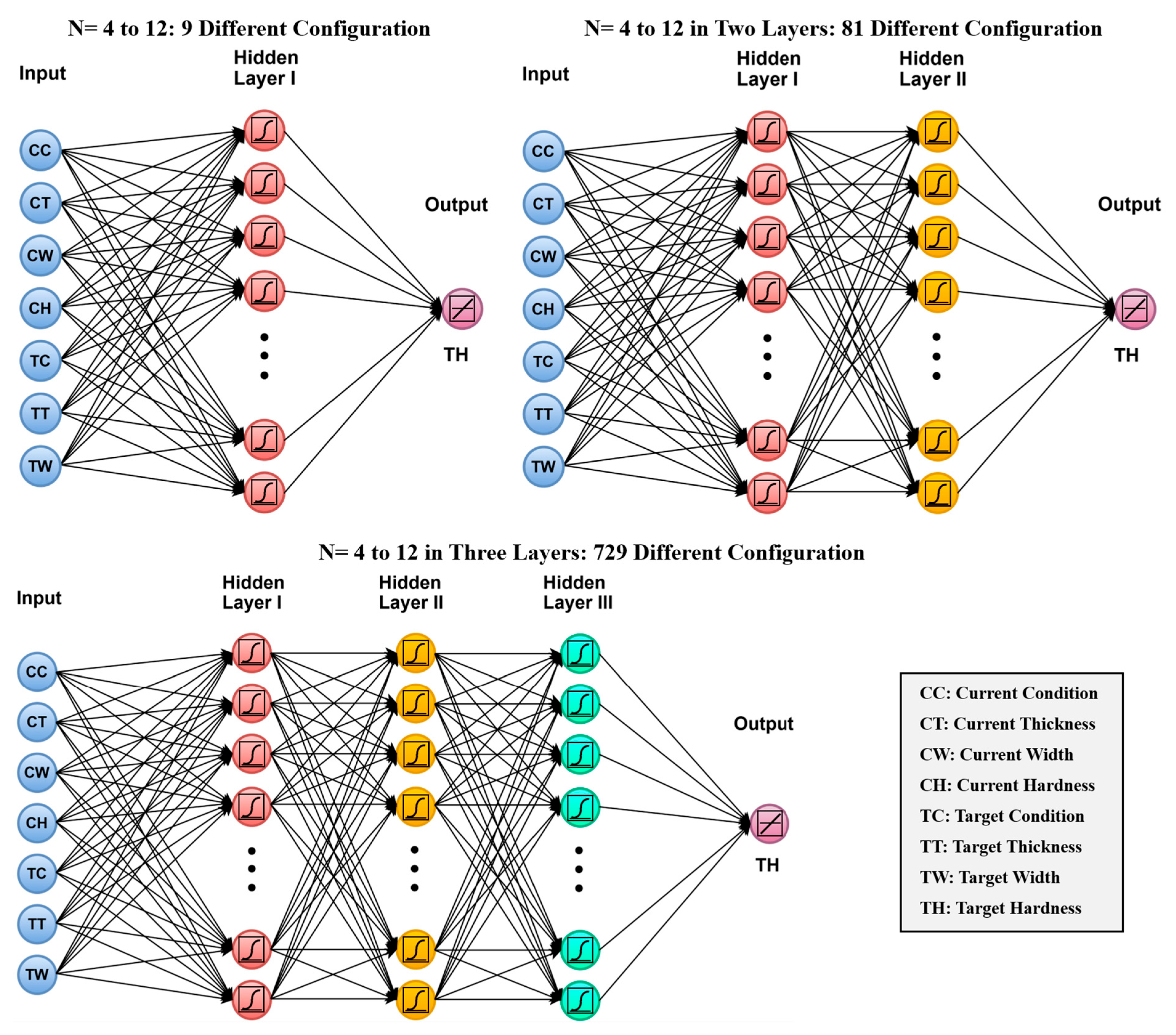
Cold rolling presents challenges due to nonlinear material deformation, fluctuating friction conditions, and strain hardening effects. Due to the complexity of predicting final material properties, ANNs are a valuable approach for capturing underlying nonlinear relationships. However, no single ANN architecture can address all requirements, as the optimal configuration depends on the type of problem being solved. This study develops multiple feedforward Rprop architectures using the logsig transfer function. Architectures with 1 to 3 hidden layers and 4 to 12 neurons in each layer were evaluated to determine the optimal configuration for predicting hardness in cold rolling, as presented in Figure 2. A total of 819 ANN architectures were evaluated, comprising 9 with one hidden layer, 81 with two hidden layers, and 729 with three hidden layers. Each architecture was trained and tested 50 times to account for the random initialization of weights and biases, ensuring comprehensive evaluation. This process resulted in a total of 40,950 simulations.
To manage the large volume of simulations and calculations in this study, we developed a MATLAB-based tool (version R2024a). This tool has been proven to offer a user-friendly framework that improves time efficiency and reduces the risk of human error associated with manual data handling and repetitive tasks [49,50]. Its application in the current work ensures consistency and reliability across all simulation steps.
In the implemented artificial intelligence (AI) framework, users can define how the dataset should be divided among the training, validation, and testing subsets. For the present investigation, the dataset was partitioned such that 70% was utilized for model training, while the remaining 30% was equally split, with 15% assigned to validation and 15% to test performance evaluation.
Rprop was chosen for this study due to its ability to effectively handle the complex, nonlinear relationships inherent in the cold rolling process. Cold rolling involves multiple interacting variables, such as rolling force, strip thickness, temperature, and material properties, leading to a highly dynamic and complex process characterized by substantial variability. Rprop is particularly well-suited for such scenarios because it adaptively adjusts weight updates based on the sign of the gradient, making it resilient to noise and varying gradients. Additionally, Rprop’s dynamic step size adjustment ensures fast and stable convergence, even with small datasets, which is critical in industrial applications where data may be limited. Its strong generalization capability and reliable performance under varying conditions make it appropriate for real-time hardness prediction in cold rolling, supporting process optimization.
The optimal number of neurons and layers in an ANN depends on the complexity of the problem, the available data, and the risk of overfitting. A higher number of neurons and layers in an ANN may improve predictions by capturing complex interactions between variables like material properties, strain, and temperature. However, too many layers and neurons may lead to overfitting, especially if the dataset is small, causing the model to memorize data rather than generalize.
A weight element in a neural network is a single learnable parameter connecting two neurons between adjacent layers, and as network complexity increases, with more neurons and weights, it demands greater computational resources and time, making real-time optimization more difficult. Therefore, balancing network complexity with problem complexity is key to effective modeling.

3. Results and Discussion

To assess the performance of the 819 developed configurations, each architecture was executed 50 times. Key performance indicators, including the R-values for training and test datasets, standard deviation (STD) of the test R-values, root mean square error (RMSE), mean absolute error (MAE), the R-value gap between training and test sets, average run time, number of epochs, and relative errors across training, validation, and test datasets were systematically computed.
In order to provide a comprehensive comparative assessment, a composite score using five distinct performance metrics, including average RMSE, average MAE, average and STD of the test R-value, the average R-value gap between training and testing data across 50 runs was calculated. Each of these metrics were assigned 20% weight and contributed equally to the composite weighted score for each architecture among others, enabling a multi-metric evaluation. Rankings were determined based on the composite score, which reflects overall model performance across all metrics.
Figure 3 illustrates the performance of ANN architectures with varying numbers of neurons in networks containing one hidden layer. The horizontal axis represents the number of hidden neurons, ranging from 4 to 12, while the left vertical axis shows the R-value, and the right vertical axis indicates the STD. The figure summarizes the average test R-value (AVG Test) and standard deviation of the test R-value (STD Test), the average training R-value (AVG Train), the maximum R-value achieved in the test data across 50 runs (Max Test), and the training R-value corresponding to the maximum test R-value (Training at Max Test).
The results demonstrate that architectures with one hidden layer exhibit consistent performance, with maximum test R-values consistently ranging between 0.96 and 0.98. The average test R-values fluctuate around 0.94, indicating good predictive performance across all configurations. Furthermore, the training R-values closely align with the test results, suggesting minimal overfitting. The architecture with 12 hidden neurons achieved the highest average R-value among all configurations, while the highest R-value in a single run was obtained with 11 hidden neurons. This indicates that increasing the number of neurons in single hidden-layer architectures improves the model’s capacity to capture the underlying complexity of the cold rolling process. The standard deviation remains relatively low (around 0.02–0.03), demonstrating that the model produces stable and reliable predictions across different training runs. The lowest STD was observed in the architecture with 12 hidden neurons. This indicates that the architecture with 12 hidden neurons provides the highest combination of accuracy and consistency.
Table 2 presents the ranking of the architectures based on the composite score, which reflects overall model performance across all evaluated metrics, providing a detailed comparative analysis of the different ANN architectures with a single hidden layer. Among the evaluated architectures, the model with 12 neurons in the hidden layer achieved the best overall performance, attaining the lowest average RMSE and MAE, along with the highest average R-value. It also exhibited a low variability in R-value and a minimal train-test R-value gap, resulting in the highest composite score and achieving the top rank. The architecture with 5 neurons demonstrated the weakest performance across all evaluated metrics. It yielded the highest RMSE and the second highest MAE, the lowest average R-value, and the largest train-test R-value gap. These deficiencies translated into the lowest composite score and last-place ranking.
Overall, the results indicate that model performance does not improve monotonically with an increasing number of neurons. While the architecture with the largest hidden layer (12 neurons) achieved the best overall performance, the model with only one fewer neuron (11 neurons) exhibited one of the weakest performances, highlighting the stochastic relationship between network size and predictive accuracy. Moreover, Table 2 reports the average relative error across the training, validation, and test datasets, offering insight into each architecture’s predictive accuracy and generalization performance. It also includes the average run time and the average number of epochs, which reflect the computational cost and convergence rate required for each model to reach an optimal solution. The top-ranked architecture (12 neurons) demonstrates the lowest relative error on the test set (3.598%), indicating superior generalization performance. Also, computational efficiency varied significantly, as the 4-neuron architecture required the shortest run time (34.223 s), but sacrificed accuracy, whereas the 12-neuron architecture demanded the longest training time (66.506 s) and the second highest number of epochs (123.36).
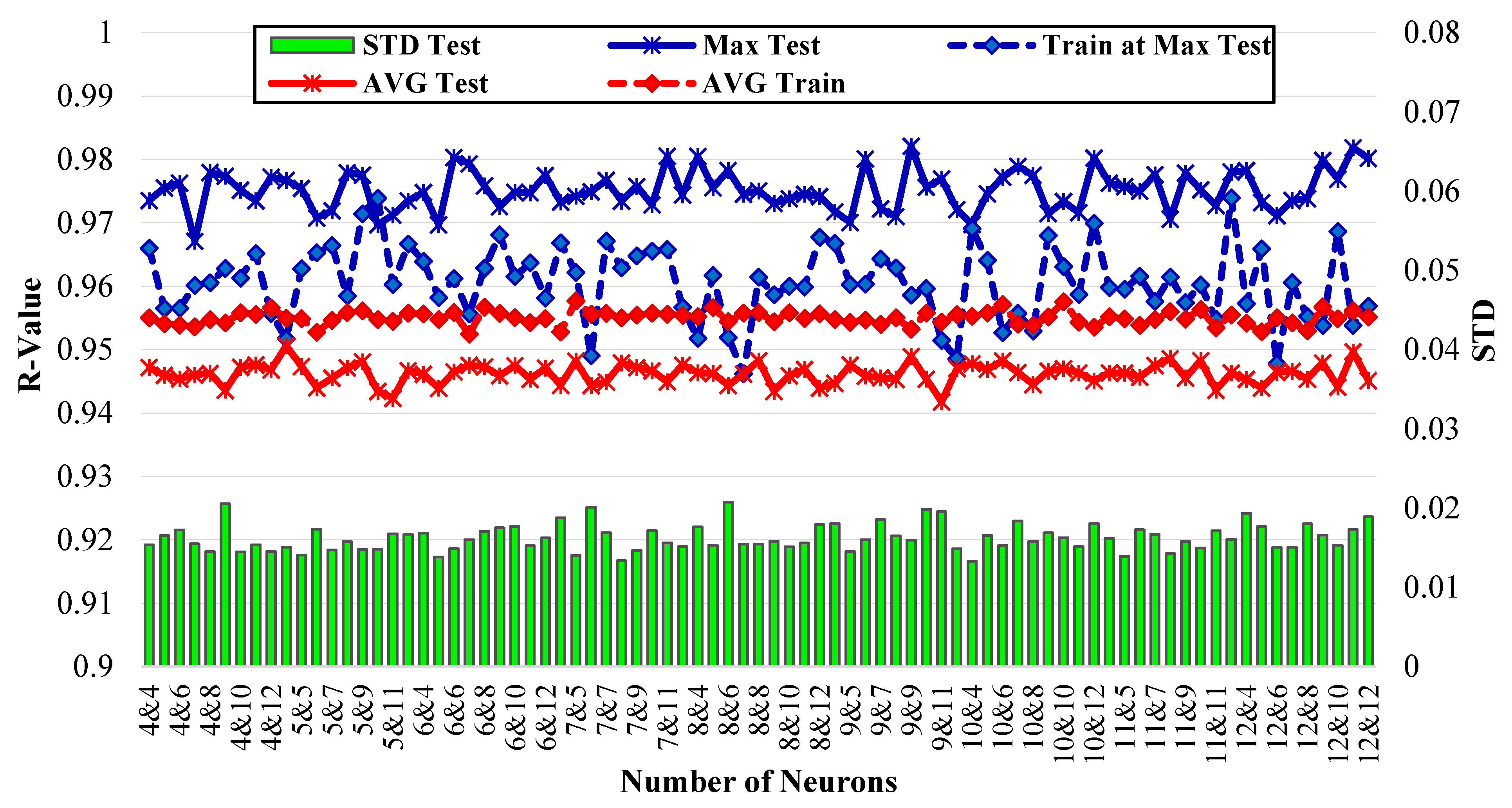
Figure 4 illustrates the performance of ANNs with two hidden layers, each evaluated over 50 runs per network architecture, where the number of neurons in the hidden layers varied from 4 to 12. The maximum test performance (Max Test) and the corresponding training performance at that peak (Train at Max Test), fluctuated around 0.95–0.98. Compared to architectures with one hidden layer, the R-values were about 1% higher which indicates that the performance of the architectures with two hidden layers was generally better than the ones with one hidden layer. Eight configurations (approximately 10% of all tested architectures) achieved maximum test R-values greater than 0.98 across 50 runs, whereas none of the configurations with a single hidden layer reached this level of accuracy. The average training and test performances remained relatively stable, with the test performance slightly lower than the training performance. Both were approximately 1% higher than those observed in architectures with a single hidden layer, indicating that two-hidden-layer architectures were better suited to capturing the complexity of the rolling process. Notably, the standard deviations were also lower than those of the single-hidden-layer architectures and remained fairly consistent across different configurations, indicating stable performance.
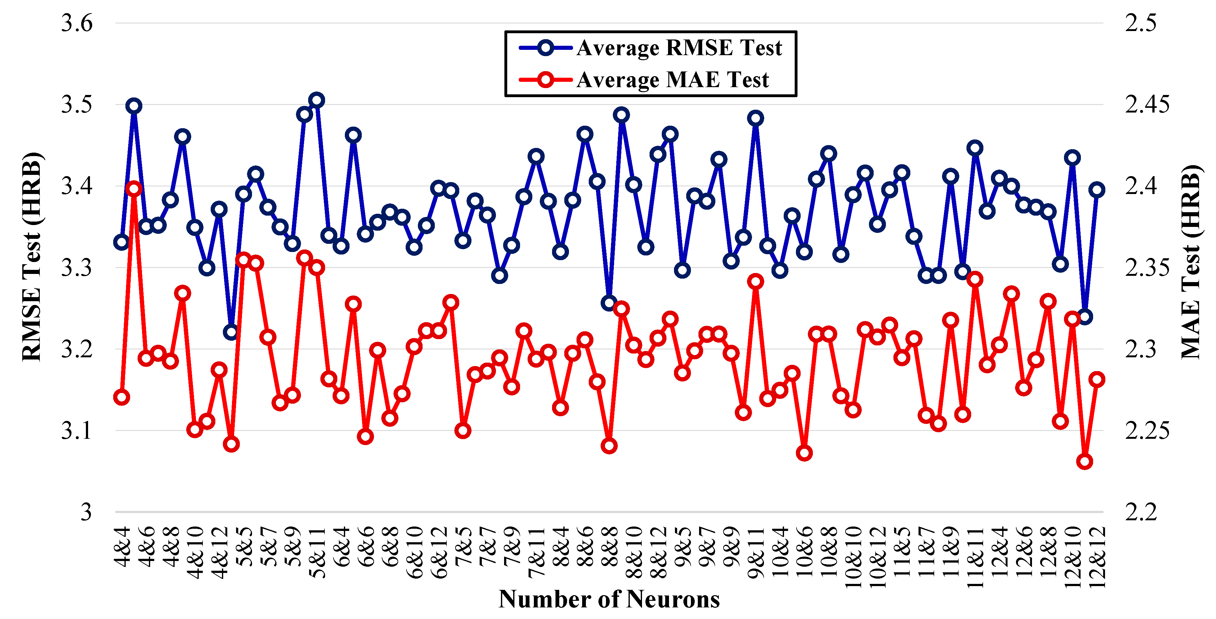
The average test RMSE and MAE results (in HRB) for all architectures with two hidden layers are presented in Figure 5. A comparative analysis of the top ten ANN architectures with two hidden layers, based on the results presented in Figure 4 and Figure 5, is provided in Table 3. Based on the composite performance score, introduction of a second hidden layer markedly improved performance, with the 5-4 architecture achieving the top rank. This architecture yielded the lowest RMSE and the highest average R-value among all configurations with two hidden layers, surpassing the best single-layer model. The improvement highlights the advantage of an additional layer, allowing the model to capture more complex data patterns. It also exhibited strong generalization, with a low train-test R-value gap and moderate STD R-value. These characteristics resulted in the highest composite performance score, positioning the model as the top-performing architecture.
It is important to highlight that the best-performing architecture (5-4), with only 9 total neurons, was among the smallest configurations evaluated, outperforming several larger models. Conversely, one of the largest architectures had the second-best performance. Efficiency-wise, the best two-layer model required fewer average epochs (78.33) and shorter run time (57.149 s) than the best single-layer model, which had an average of 123.36 epochs and a run time of 66.506 s, reflecting faster convergence. The average relative error on the test dataset was 3.386%, which is lower than that of the best-performing single-layer model (3.598%), indicating the superior performance of two-layer architectures for this dataset.
These results emphasize the importance of evaluating the predictive accuracy of each architecture individually and conducting architecture optimization, as relying solely on model size as an indicator of performance can be misleading. An increase in architecture size did not guarantee better performance, as no consistent correlation was identified between model complexity and predictive performance. Even when a couple of architectures achieve comparable performance, the simplest should be selected to maintain computational efficiency and reduce the risk of overfitting [51].
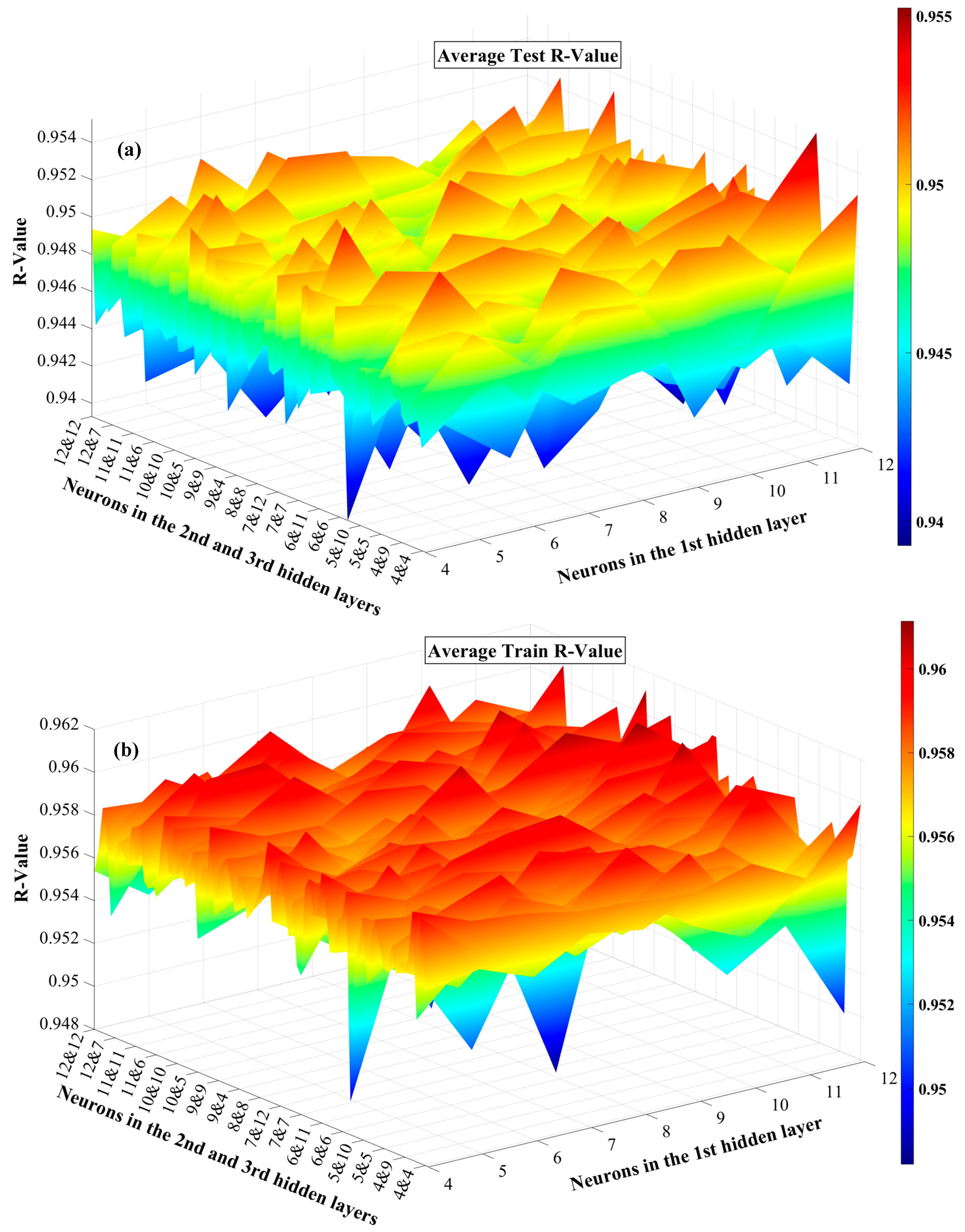
Figure 6 and Figure 7 present 3D surface plots illustrating the average performance metrics, including R-value, RMSE, and MAE, across 50 independent runs for various ANN architectures with three hidden layers. The horizontal axis on the right in the 3D plots represents the number of neurons in the first hidden layer, while the left horizontal axis represents the number of neurons in the second and third hidden layers. In Figure 6, the color scale on the right provides a visual representation of R-values, with red indicating higher values and blue representing lower ones. The dataset corresponding to this figure is included in Appendix A. Figure 6a shows that the network generally maintains average R-values between 0.940 and 0.955 on the test data, with limited fluctuation. Some variation in performance is observed across different configurations, with certain neuron structures yielding slightly higher average R-values, as shown by the red regions. This suggests that while increasing the number of neurons enhanced performance in some cases, it does not guarantee consistent improvements. Additionally, Figure 6b, which shows the average R-values for the training dataset, exhibits a narrower fluctuation range, 0.950 to 0.960, compared to that of the test data. The training average R-values were generally higher than those of the test data, indicating that the model fits the training data with higher consistency and accuracy. Moreover, higher train R-values (Figure 6b) are more uniformly distributed across architectures, while test R-values (Figure 6a) show greater variability, highlighting the sensitivity of model generalization to architectural choices.
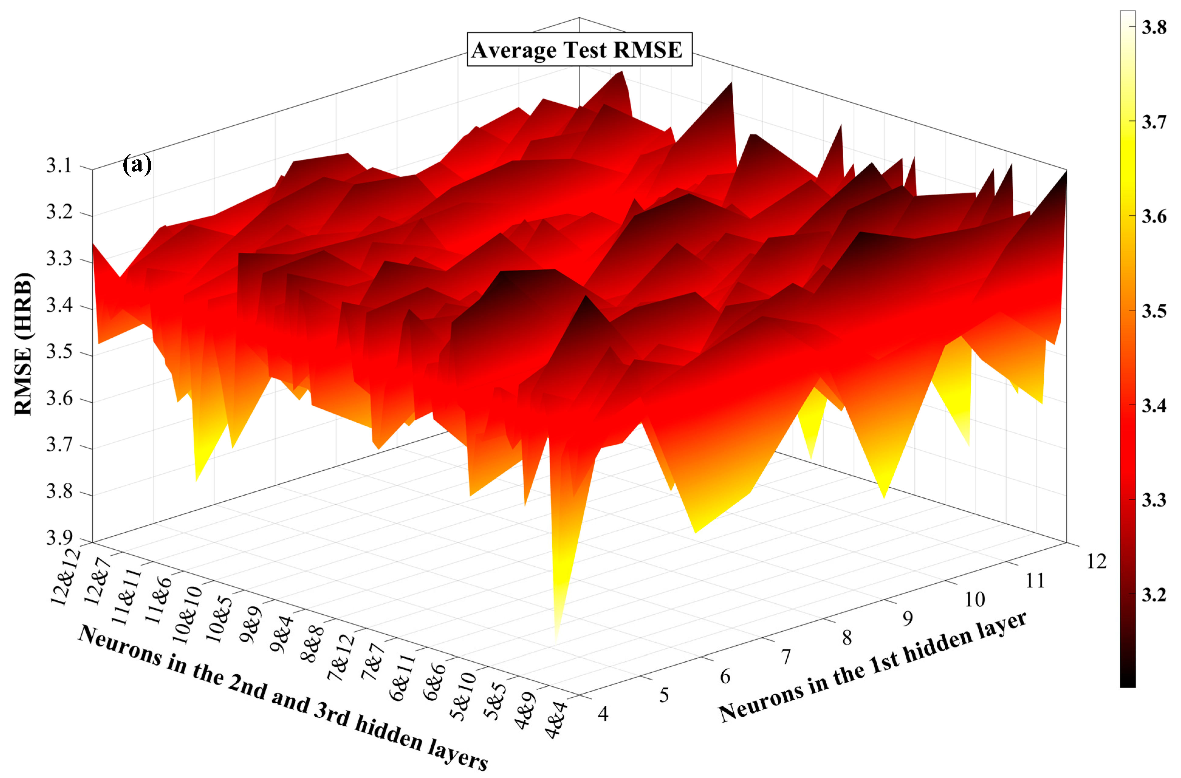
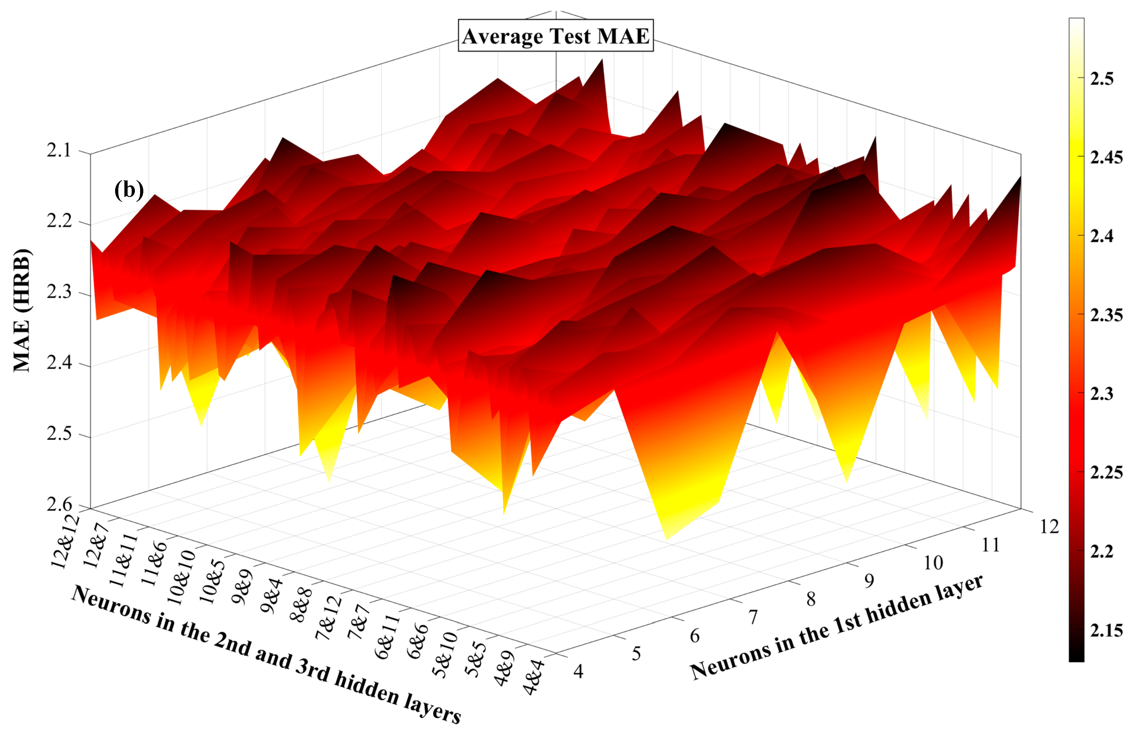
Figure 7a,b present 3D surface plots illustrating the average test performance of various three-hidden-layer ANN architectures in terms of RMSE and MAE, respectively, providing a comprehensive comparison across a wide range of neuron configurations. Given that both RMSE and MAE are error metrics where lower values represent better predictive performance, the Z-axis is inverted to better demonstrate the inverse relationship between error magnitude and model performance. Across both plots, the performance surfaces exhibit noticeable local minima and gradients, indicating that network performance is sensitive to architectural configuration. Architectures with lower average RMSE and MAE correspond closely to those with higher R-values, confirming the consistency of evaluation metrics.
Table 4 presents a comparative evaluation of the top ten ANN architectures with three hidden layers, ranked by their composite scores. Among the tested configurations, the 12-5-5 architecture achieved the best overall performance, ranking first with the highest composite score. It also demonstrated the highest average R-value on the test set and a small train-test R-value gap of 0.001, indicating strong predictive accuracy and minimal overfitting. It is worth noting that the top three architectures, 12-5-5, 12-4-4, and 12-5-7, ranked best among 729 configurations, and all share a closely similar architecture with the largest number of neurons in the first hidden layer, followed by much smaller numbers in the second and third layers. This pattern likely enables effective hidden pattern detection early in the network while maintaining simplicity in the deeper layers, leading to improved generalization.
The top-ranked three-layer architecture converged with a lower average number of epochs (61.74) than the best-performing one- and two-layer models. However, its average run time (73.663 s) was longer than that of the one- and two-layer models due to the increased computational complexity introduced by the additional hidden layer.
The performance comparison of top-ranked ANN architectures with one, two, and three hidden layers highlights key trends in model behavior. The best single-layer network (12 neurons) yields an RMSE of 3.498, MAE of 2.465, and R-value of 0.941, serving as a performance baseline. Adding a second hidden layer, the accuracy of the best two-layer model (5-4) significantly improved, reducing RMSE to 3.221 and MAE to 2.242, and improving the R-value to 0.951. Extending to three hidden layers, the top-performing model (12-5-5) marginally reduced RMSE to 3.201 and slightly increased the R-value to 0.955; however, MAE rose to 2.315. While the transition from one to two layers consistently improved all three metrics, adding a third layer yielded only marginal gains in RMSE and R-value, but a higher MAE, suggesting diminishing returns and a potential trade-off between accuracy and generalization. Notably, the small gap between training and test relative errors across top-performing models suggests that overfitting was effectively mitigated through Rprop and tuning of network architectures.
In many recent studies, the maximum test R-values have been regarded as key error parameters in the selection of the best-performing architecture. Considering this, a separate comparison based on R-values was conducted to identify the best single simulation run, thereby enabling a direct comparison of the highest achieved R-value with those reported in other studies. In addition to the R-value, it is essential to monitor the difference between the training and testing R-values, ensuring it remains minimal to reduce the risk of overfitting.
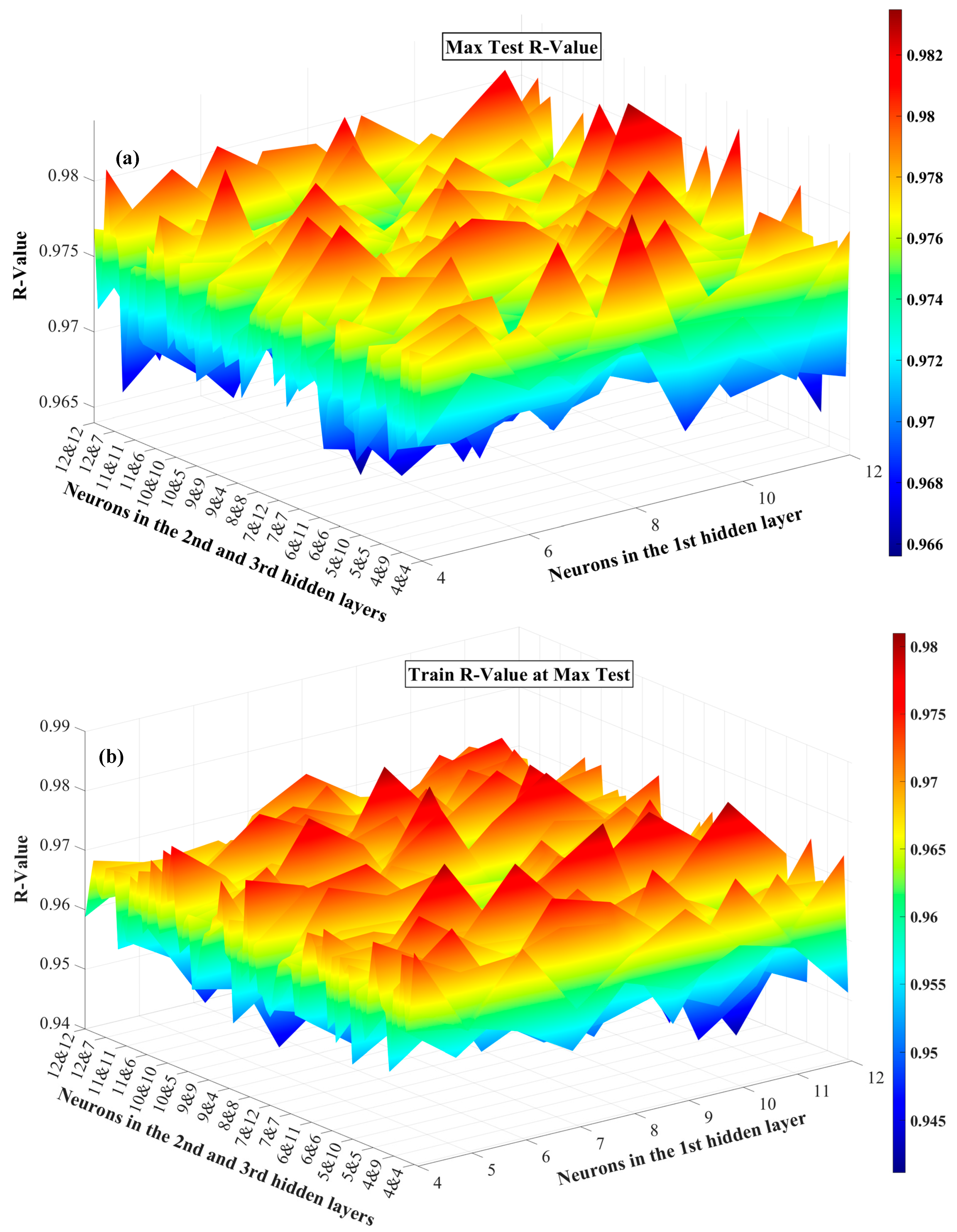
Figure 8 shows a 3D surface plot illustrating the maximum test R-values along with their corresponding training R-values for ANN architectures with three hidden layers, with the data detailed in the Appendix A. The presence of peaks in the red regions suggests that certain architectures significantly outperform others, while the blue regions indicate configurations with weaker generalization. As shown in Figure 8a, 27 architectures, approximately 3.7% of the configurations, achieved R-values above 0.98, which is lower than the proportion observed in the two-hidden-layer case (~10%). The maximum R-value in this case, 0.9835, was achieved by the 11-8-9 architecture. Figure 8b illustrates that similar to the two-hidden-layer configurations, the test R-values at peak performance exceed their corresponding training R-values. However, the overall performance of the three-hidden-layer architectures showed minimal improvement compared to the two-hidden-layer models, suggesting that increased complexity does not necessarily enhance performance. Additionally, it was revealed that some configurations with higher number of neurons such as 11 or 12 neurons in the first layer achieve slightly higher R values (e.g., 0.9835, 0.9826, 0.9825), compared to others; however, these peaks are not consistent enough to declare a clear trend favoring larger networks.
The details of the architectures with the best single run (based on R-value) in one-, two-, and three-layer architectures are presented in Table 5. It shows that the architecture within the two-hidden-layer configuration performed better than the one-hidden-layer model, while the best three-hidden-layer architecture shows much smaller improvement in R-values than the two-hidden-layer configuration. These results are consistent with those in composite scores.
Table 5 also provides a detailed comparison of the complexity of the best run ANN architectures with one, two, and three hidden layers. As the number of layers increases, architectures with the best single run consequently grow significantly in size in each case. The one-layer network has 11 neurons and 109 weight elements, the two-layer model expands to 18 neurons and 265 weight elements, and the three-layer configuration reaches 28 neurons and 421 weight elements. This escalation reflects a notable increase in model complexity. To evaluate the statistical reliability of the neural network predictions, paired t-tests were conducted to compare the predicted and actual values for each architecture. The resulting p-values for the best-performing 1-layer, 2-layer, and 3-layer networks were 0.424, 0.329, and 0.392, respectively, all above the 0.05 significance threshold, meaning that there is no statistically significant difference between the predicted and actual values, suggesting that the models’ predictions are consistent with the true data and that the observed prediction accuracy is not due to random chance.
Figure 9 shows scatter plots of actual versus predicted values for ANN models with one, two, and three hidden layers, corresponding to the architectures detailed in Table 5. These plots illustrate the predictive performance of each configuration by indicating the degree of agreement between the predicted and actual values across the training, validation, and test datasets. In all three configurations, the predicted outputs closely align with the actual data points across training, validation, and test sets, demonstrating the overall effectiveness of the ANNs in capturing the underlying data relationships. The clustering of points near the diagonal indicates good prediction accuracy. The two-hidden-layer and the three-hidden-layer architectures show tighter clustering around the diagonal line relative to the one-hidden-layer architecture, implying improved model fitting and reduced prediction error. However, noticeable dispersion occurs in regions with sparse data, indicating variability and potential underfitting. This suggests that the model may not fully capture the underlying data patterns in this region.

4. Conclusions

This study presented a comparative analysis of Rprop-based ANNs to evaluate the influence of hidden layers and the number of neurons on hardness prediction in the cold rolling of 70-30 brass, aiming to address challenges arising from the nonlinear deformation and strain hardening inherent in the process. Dimensional and hardness measurements collected across multiple rolling passes were used to develop and validate the ANN models. The results compare the predictive performance of different ANN configurations and highlight their effectiveness in capturing complex relationships within the data, offering insights into the impact of network architecture on model accuracy. Specimens underwent multiple rolling passes, during which dimensional and hardness measurements were recorded. A dataset comprising 1000 input–output pairs was used to develop and evaluate 819 different Rprop-based ANN architectures, including one to three hidden layers with 4 to 12 neurons per layer. Each network architecture was trained and evaluated across 50 independent runs to mitigate the effects of random initialization and training variability and to ensure consistency and reliability in the results.
A composite score using five performance metrics, including averages of RMSE, MAE, test R-value and its STD, and the R-value gap between training and testing over 50 runs, was calculated for comprehensive comparison. The results demonstrated that the number of hidden layers directly influenced the predictive performance of the ANN model; however, increasing the number beyond a certain point may result in diminishing returns. The results showed that the best single-layer network (12 neurons) sets the baseline with RMSE 3.498, MAE 2.465, and R-value 0.941. Adding a second layer, the top model (5-4) improved accuracy with RMSE 3.221, MAE 2.242, and R-value 0.951. The three-layer model (12-5-5) slightly reduced RMSE to 3.201 and raised R-value to 0.955, but MAE increased to 2.315. Therefore, introducing a third hidden layer did not lead to meaningful improvement in the performance metrics when compared to the two-hidden-layer architectures. Moreover, the top-ranked three-layer architecture converged in fewer epochs on average (61.74) than the best one- and two-layer architectures but had a longer average run time (73.663 s) due to the added computational complexity.

Author Contributions

Conceptualization, E.S. and F.K.; methodology, E.S. and F.K.; software, E.S. and F.K.; validation, E.S. and F.K.; formal analysis, E.S. and F.K.; investigation, E.S., F.K. and S.F.M.; resources, S.F.M.; data curation, E.S., F.K. and S.F.M.; writing—original draft preparation, E.S., F.K. and S.F.M.; writing—review and editing, E.S., F.K. and S.F.M.; visualization, E.S. and F.K.; supervision, E.S. and F.K.; funding acquisition, S.F.M. All authors have read and agreed to the published version of the manuscript.

Funding

This investigation was supported by NSF CMMI grant # 1763147 and Office of Naval Research award # N000142112861.

Conflicts of Interest

The authors declare no conflict of interest.

Appendix A

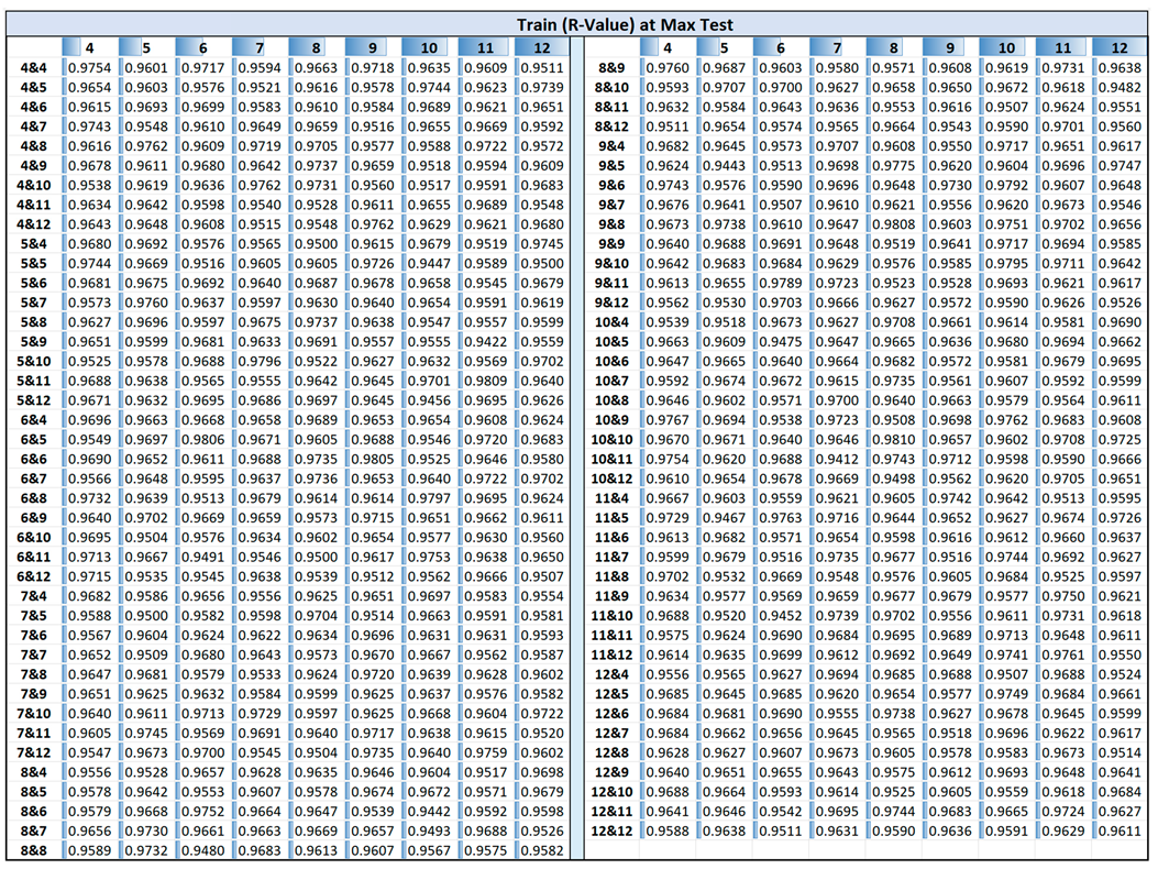
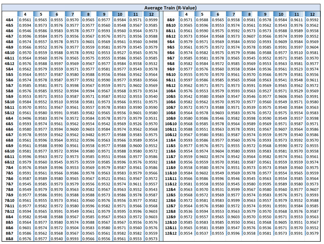
Appendix A summarizes data including maximum test R-values, training R-values at maximum test, average test R-values, and average training R-values across 50 simulation runs for each unique network within the three-hidden-layer structures:
Jmmp 09 00260 i001Jmmp 09 00260 i002Jmmp 09 00260 i003Jmmp 09 00260 i004

References

  1. Mumali, F. Artificial neural network-based decision support systems in manufacturing processes: A systematic literature review. Comput. Ind. Eng. 2022, 165, 107964. [Google Scholar] [CrossRef]
  2. Adil, M.; Ullah, R.; Noor, S.; Gohar, N. Effect of number of neurons and layers in an artificial neural network for generalized concrete mix design. Neural Comput. Appl. 2022, 34, 8355–8363. [Google Scholar] [CrossRef]
  3. Keskin, F.D.; Çiçekli, U.; İçli, D. Prediction of failure categories in plastic extrusion process with deep learning. J. Intell. Syst. Theory Appl. 2022, 5, 27–34. [Google Scholar] [CrossRef]
  4. Ghnatios, C.; Gravot, E.; Champaney, V.; Verdon, N.; Hascoët, N.; Chinesta, F. Polymer extrusion die design using a data-driven autoencoders technique. Int. J. Mater. Form. 2024, 17, 4. [Google Scholar] [CrossRef]
  5. Mrzygłód, B.; Hawryluk, M.; Janik, M.; Wożeńska, I.O. Sensitivity analysis of the artificial neural networks in a system for durability prediction of forging tools to forgings made of C45 steel. Int. J. Adv. Manuf. Technol. 2020, 109, 1385–1395. [Google Scholar] [CrossRef]
  6. Mrzygłód, B.; Hawryluk, M.; Gronostajski, Z.; Opaliński, A.; Kaszuba, M.; Polak, S.; Widomski, P.; Ziemba, J.; Zwierzchowski, M. Durability analysis of forging tools after different variants of surface treatment using a decision-support system based on artificial neural networks. Arch. Civ. Mech. Eng. 2018, 18, 1079–1091. [Google Scholar] [CrossRef]
  7. Lee, S.; Kim, K.; Kim, N. A Preform Design Approach for Uniform Strain Distribution in Forging Processes Based on Convolutional Neural Network. J. Manuf. Sci. Eng. 2022, 144, 121004. [Google Scholar] [CrossRef]
  8. Yuan, C.; Ling, Y.; Zhang, N.; Yang, Y.; Pan, L.; Han, C.; Cao, Y.; Zhang, H.; Nie, P.; Ma, H. Fault Diagnosis Method of Forging Press Based on Improved CNN. IEEE Access 2024, 12, 181925–181936. [Google Scholar] [CrossRef]
  9. Naranje, V.; Kumar, S.; Kashid, S.; Ghodke, A.; Hussein, H.M.A. Prediction of life of deep drawing die using artificial neural network. Adv. Mater. Process. Technol. 2016, 2, 132–142. [Google Scholar] [CrossRef]
  10. Sevsek, L.; Vilkovsky, S.; Majerníková, J.; Pepelnjak, T. Predicting the deep drawing process of TRIP steel grades using multilayer perceptron artificial neural networks. Adv. Prod. Eng. Manag. 2024, 19, 46–64. [Google Scholar] [CrossRef]
  11. Manoochehri, M.; Kolahan, F. Integration of artificial neural network and simulated annealing algorithm to optimize deep drawing process. Int. J. Adv. Manuf. Technol. 2014, 73, 241–249. [Google Scholar] [CrossRef]
  12. El Mrabti, I.; Touache, A.; El Hakimi, A.; Chamat, A. Springback optimization of deep drawing process based on FEM-ANN-PSO strategy. Struct. Multidiscip. Optim. 2021, 64, 321–333. [Google Scholar] [CrossRef]
  13. Liu, S.; Xia, Y.; Shi, Z.; Yu, H.; Li, Z.; Lin, J. Deep Learning in Sheet Metal Bending with a Novel Theory-Guided Deep Neural Network. IEEE/CAA J. Autom. Sin. 2021, 8, 565–581. [Google Scholar] [CrossRef]
  14. Sahib, M.M.; Kovács, G. Using Artificial Neural Networks to Predict the Bending Behavior of Composite Sandwich Structures. Polymers 2025, 17, 337. [Google Scholar] [CrossRef]
  15. Nguyen, T.N.; Zhang, D.; Mirrashid, M.; Nguyen, D.K.; Singhatanadgid, P. Fast analysis and prediction approach for geometrically nonlinear bending analysis of plates and shells using artificial neural networks. Mech. Adv. Mater. Struct. 2023, 31, 10221–10239. [Google Scholar] [CrossRef]
  16. Xu, B.; Li, L.; Wang, Z.; Zhou, H.; Liu, D. Prediction of springback in local bending of hull plates using an optimized backpropagation neural network. Mech. Sci. 2021, 12, 777–789. [Google Scholar] [CrossRef]
  17. Thakur, S.K.; Das, A.K.; Jha, B.K. Application of machine learning methods for the prediction of roll force and torque during plate rolling of micro-alloyed steel. J. Alloys Metall. Syst. 2023, 4, 100044. [Google Scholar] [CrossRef]
  18. Yang, Y.Y.; Linkens, D.A.; Talamantes-Silva, J.; Howard, I.C. Roll Force and Torque Prediction Using Neural Network and Finite Element Modelling. ISIJ Int. 2003, 43, 1957–1966. [Google Scholar] [CrossRef]
  19. Hwang, R.; Jo, H.; Kim, K.S.; Hwang, H.J. Hybrid Model of Mathematical and Neural Network Formulations for Rolling Force and Temperature Prediction in Hot Rolling Processes. IEEE Access 2020, 8, 153123–153133. [Google Scholar] [CrossRef]
  20. Rath, S.; Sengupta, P.P.; Singh, A.P.; Marik, A.K.; Talukdar, P. Mathematical-artificial neural network hybrid model to predict roll force during hot rolling of steel. Int. J. Comput. Mater. Sci. Eng. 2013, 2, 1350004. [Google Scholar] [CrossRef]
  21. Yang, Y.Y.; Linkens, D.A.; Talamantes-Silva, J. Roll load prediction-data collection, analysis and neural network modelling. J. Mater. Process. Technol. 2004, 152, 304–315. [Google Scholar] [CrossRef]
  22. Xia, J.S.; Khabaz, M.K.; Patra, I.; Khalid, I.; Alvarez, J.R.N.; Rahmanian, A.; Eftekhari, S.A.; Toghraie, D. Using feed-forward perceptron Artificial Neural Network (ANN) model to determine the rolling force, power and slip of the tandem cold rolling. ISA Trans. 2023, 132, 353–363. [Google Scholar] [CrossRef]
  23. Ostasevicius, V.; Paleviciute, I.; Paulauskaite-Taraseviciene, A.; Jurenas, V.; Eidukynas, D.; Kizauskiene, L. Comparative Analysis of Machine Learning Methods for Predicting Robotized Incremental Metal Sheet Forming Force. Sensors 2022, 22, 18. [Google Scholar] [CrossRef] [PubMed]
  24. Zárate, L.E. A method to determinate the thickness control parameters in cold rolling process through predictive model via neural networks. J. Braz. Soc. Mech. Sci. Eng. 2005, 27, 357–363. [Google Scholar] [CrossRef]
  25. Wang, H.Y.; Huang, C.Q.; Deng, H. Prediction on Transverse Thickness of Hot Rolling Aluminum Strip Based on BP Neural Network. In Applied Mechanics and Materials; Trans Tech Publications, Ltd.: Bäch, Switzerland, 2012; Volume 157–158, pp. 78–83. [Google Scholar]
  26. Hou, C.K.J.; Behdinan, K. Neural networks with dimensionality reduction for predicting temperature change due to plastic deformation in a cold rolling simulation. AI EDAM 2023, 37, e1. [Google Scholar] [CrossRef]
  27. Ding, C.Y.; Ye, J.C.; Lei, J.W.; Wang, F.F.; Li, Z.Y.; Peng, W.; Zhang, D.H.; Sun, J. An interpretable framework for high-precision flatness prediction in strip cold rolling. J. Mater. Process. Technol. 2024, 329, 118452. [Google Scholar] [CrossRef]
  28. Zhao, J.; Li, J.; Qie, H.; Wang, X.; Shao, J.; Yang, Q. Predicting flatness of strip tandem cold rolling using a general regression neural network optimized by differential evolution algorithm. Int. J. Adv. Manuf. Technol. 2023, 126, 3219–3233. [Google Scholar] [CrossRef]
  29. Smetana, M.; Gala, M.; Gombarska, D.; Klco, P. Neural Network-Based Evaluation of Hardness in Cold-Rolled Austenitic Stainless Steel Under Various Heat Treatment Conditions. Appl. Sci. 2025, 15, 1352. [Google Scholar] [CrossRef]
  30. Cui, C.; Cao, G.; Li, X.; Gao, Z.; Liu, J.; Liu, Z. A strategy combining machine learning and physical metallurgical principles to predict mechanical properties for hot rolled Ti micro-alloyed steels. J. Mater. Process. Technol. 2023, 311, 117810. [Google Scholar] [CrossRef]
  31. Ghaisari, J.; Jannesari, H.; Vatani, M. Artificial neural network predictors for mechanical properties of cold rolling products. Adv. Eng. Softw. 2012, 45, 91–99. [Google Scholar] [CrossRef]
  32. Xu, Z.W.; Liu, X.M.; Zhang, K. Mechanical Properties Prediction for Hot Rolled Alloy Steel Using Convolutional Neural Network. IEEE Access 2019, 7, 47068–47078. [Google Scholar] [CrossRef]
  33. Xie, Q.; Suvarna, M.; Li, J.; Zhu, X.; Cai, J.; Wang, X. Online prediction of mechanical properties of hot rolled steel plate using machine learning. Mater. Des. 2021, 197, 109201. [Google Scholar] [CrossRef]
  34. Li, X.; Luan, F.; Wu, Y. A Comparative Assessment of Six Machine Learning Models for Prediction of Bending Force in Hot Strip Rolling Process. Metals 2020, 10, 685. [Google Scholar] [CrossRef]
  35. Stathakis, D. How many hidden layers and nodes? Int. J. Remote Sens. 2009, 30, 2133–2147. [Google Scholar] [CrossRef]
  36. Abdolrasol, M.G.M.; Hussain, S.M.S.; Ustun, T.S.; Sarker, M.R.; Hannan, M.A.; Mohamed, R.; Ali, J.A.; Mekhilef, S.; Milad, A. Artificial Neural Networks Based Optimization Techniques: A Review. Electronics 2021, 10, 2689. [Google Scholar] [CrossRef]
  37. Murugesan, M.; Sajjad, M.; Jung, D.W. Hybrid Machine Learning Optimization Approach to Predict Hot Deformation Behavior of Medium Carbon Steel Material. Metals 2019, 9, 1315. [Google Scholar] [CrossRef]
  38. Sheela KGnana Deepa, S.N. Review on methods to fix number of hidden neurons in neural networks. Math. Probl. Eng. 2013, 1, 425740. [Google Scholar]
  39. Heaton, J. Introduction to Neural Networks with Java; Heaton Research, Inc.: Chesterfield, MO, USA, 2008. [Google Scholar]
  40. Merayo, D.; Rodríguez-Prieto, A.; Camacho, A.M. Topological Optimization of Artificial Neural Networks to Estimate Mechanical Properties in Metal Forming Using Machine Learning. Metals 2021, 11, 1289. [Google Scholar] [CrossRef]
  41. Contreras-Fortes, J.; Rodríguez-García, M.I.; Sales, D.L.; Sánchez-Miranda, R.; Almagro, J.F.; Turias, I.A. Machine Learning Approach for Modelling Cold-Rolling Curves for Various Stainless Steels. Materials 2024, 17, 147. [Google Scholar] [CrossRef]
  42. Gorji, M.B.; Mohr, D. Towards neural network models for describing the large deformation behavior of sheet metal. IOP Conf. Ser. Mater. Sci. Eng. 2019, 651, 012102. [Google Scholar] [CrossRef]
  43. Byun, S.; Yu, J.; Cheon, S.; Lee, S.H.; Park, S.H.; Lee, T. Enhanced prediction of anisotropic deformation behavior using machine learning with data augmentation. J. Magnes. Alloys 2024, 12, 186–196. [Google Scholar] [CrossRef]
  44. Gerlach, J.; Schulte, R.; Schowtjak, A.; Clausmeyer, T.; Ostwald, R.; Tekkaya, A.E.; Menzel, A. Enhancing damage prediction in bulk metal forming through machine learning-assisted parameter identification. Arch. Appl. Mech. 2024, 94, 2217–2242. [Google Scholar] [CrossRef]
  45. Hawkins, D.M. The problem of overfitting. J. Chem. Inf. Comput. Sci. 2004, 44, 1–12. [Google Scholar] [CrossRef]
  46. Goodfellow, I.; Bengio, Y.; Courville, A. Deep Learning; The MIT Press: Cambridge, MA, USA, 2016; ISBN 978-0262035613. [Google Scholar]
  47. Kaplan, J.; McCandlish, S.; Henighan, T.; Brown, T.B.; Chess, B.; Child, R.; Gray, S.; Radford, A.; Wu, J.; Amodei, D. Scaling laws for neural language models. arXiv 2020, arXiv:2001.08361. [Google Scholar]
  48. MatWeb. Available online: https://www.matweb.com/ (accessed on 10 June 2025).
  49. Seidi, E.; Miller, S.F.; Kaviari, F.; Huang, L.; Stoughton, T.B. Novel method to assess anisotropy in formability using DIC. Int. J. Mech. Sci. 2025, 285, 109782. [Google Scholar] [CrossRef]
  50. Seidi, E.; Miller, S.; Huang, L.; Stoughton, T. Mathematical Analysis of the Tensile Behavior of DP 980 Steel Using Digital Image Correlation (DIC). ASME Int. Manuf. Sci. Eng. Conf. 2023, 87240, V002T06A038. [Google Scholar]
  51. Hagan, M.T.; Demuth, H.B.; Beale, M.H.; Jesús, O.D. Neural Network Design, 2nd ed.; E-book; PWS Publishing Co.: Hornsea, UK, 2014; Available online: https://hagan.okstate.edu/nnd.html (accessed on 10 June 2025).
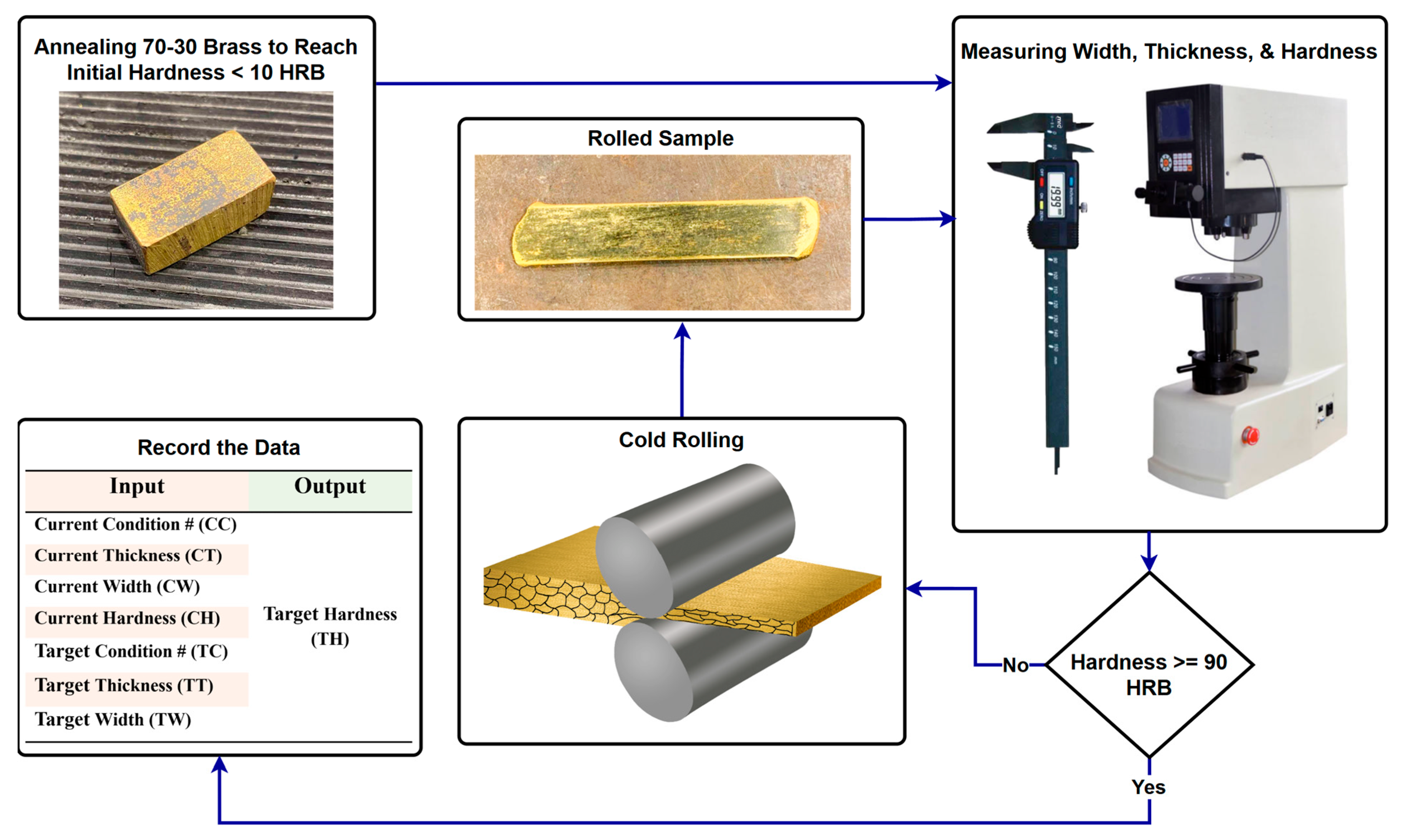
Figure 1. Experimental procedure for generating a large dataset to evaluate ANN structures.
Jmmp 09 00260 g001
Figure 2. ANN architectures with one, two, and three hidden layers used for predicting hardness based on seven input features after a specific number of rolls and thickness reduction.
Jmmp 09 00260 g002
Figure 3. Performance measurements of architectures with one hidden layer for varying numbers of neurons.
Jmmp 09 00260 g003
Figure 4. Performance measurements of architectures with two hidden layers.
Jmmp 09 00260 g004
Figure 5. Average RMSE and MAE on test data for architectures with two hidden layers (lower values indicate better performance).
Jmmp 09 00260 g005
Figure 6. Average R-values of (a) test and (b) train datasets in the three hidden layer architectures across 50 runs.
Jmmp 09 00260 g006
Figure 7. Average test (a) RMSE and (b) MAE in the three hidden layer architectures across 50 runs.
Jmmp 09 00260 g007aJmmp 09 00260 g007b
Figure 8. (a) Maximum test R-values and (b) corresponding train R-values across 50 runs for three-hidden-layer architectures.
Jmmp 09 00260 g008
Figure 9. Performance comparison of ANNs with max R-value in architectures with (a) one, (b) two, and (c) three hidden layers.
Jmmp 09 00260 g009
Table 1. The elemental composition, mechanical, and thermal properties of 70-30 brass [48].
Elements:CuZnFePbAll Other Elements
68.5–71.5%28.5–31.5%≤0.050%≤0.070%≤0.15%
Mechanical propertiesYield
Stress
UTSYoung’s ModulusPoisson’s RatioElongation at Break
95 MPa315 MPa110 GPa0.37565%
Thermal propertiesLiquidusSolidusSpecific Heat
Capacity
Thermal
Conductivity
Coefficient of
Thermal Expansion
955 °C915 °C0.375 J/g-°C120 W/m-K19.9 µm/m-°C
Table 2. Performance rank and metrics of ANN architectures with one hidden layer, varying by neuron count.
RankStructureAvg. RMSE TestAvg. MAE TestAvg. R-Value TestSTD R-Value TestTrain-Test R-Value GapAvg. Run TimeAvg. Num. of EpochAvg. Rel. Error TrainAvg. Rel. ErrorValidationAvg. Rel. Error Test
1123.4982.4650.9410.0170.00466.506123.363.972%3.4796%3.598%
2103.5562.5210.9390.0190.00363.026109.883.921%4.2868%3.656%
383.6762.5700.9380.0190.00755.809119.483.774%4.1852%4.061%
443.7062.5740.9380.0200.00634.223122.043.729%4.5739%4.212%
573.7232.5310.9380.0210.00750.068110.33.713%3.8558%4.595%
663.7162.5420.9350.0210.00847.129107.543.950%3.6053%4.213%
793.6752.5190.9370.0260.00860.671125.583.772%3.6189%4.281%
8113.6852.5970.9340.0240.00864.222104.023.835%4.5527%3.926%
953.8702.5890.9320.0190.01241.815111.963.722%3.8279%4.941%
Table 3. Performance rank and metrics of ANN architectures with two hidden layers, varying by neuron count.
RankStructureAvg. RMSE TestAvg. MAE TestAvg. R-Value TestSTD R-Value TestTrain-Test R-Value GapAvg. Run TimeAvg. Num. of EpochAvg. Rel. Error TrainAvg. Rel. ErrorValidationAvg. Rel. Error Test
15-43.2212.2420.9510.0150.00457.14978.333.396%3.990%3.386%
212-113.2392.2310.9500.0170.00749.34084.873.368%3.576%3.559%
311-83.2902.2540.9490.0140.00750.38785.853.335%3.872%3.628%
48-83.2562.2410.9480.0160.00883.60884.753.375%3.655%3.491%
510-43.2962.2750.9480.0130.00855.28686.923.430%3.715%3.373%
69-93.3082.2970.9490.0160.00462.90173.43.528%3.357%3.426%
77-83.2902.2950.9480.0130.00776.45278.613.335%4.469%3.245%
811-103.2952.2600.9480.0150.00850.41080.043.326%3.775%3.528%
99-53.2972.2850.9480.0150.00787.57477.633.399%4.110%3.432%
1010-63.3192.2360.9480.0150.00953.32784.263.262%3.840%3.750%
Table 4. Performance metrics and ranking of ANN architectures with three hidden layers, varying by neuron count.
Rank Structure Avg. RMSE Test Avg. MAE Test Avg. R-Value Test STD R-Value Test Train-Test R-Value Gap Avg. Run Time Avg. Num. of Epoch Avg. Rel. Error Train Avg. Rel. Error
Validation
Avg. Rel. Error Test
112-5-53.2012.3150.9550.0140.00173.66361.743.648%4.067%3.024%
212-4-43.1012.1290.9530.0120.00773.70069.443.141%3.873%3.230%
312-5-73.1452.1730.9530.0140.00473.51369.523.314%3.377%3.326%
45-5-43.1192.1790.9530.0140.00578.21868.93.275%3.763%3.008%
511-5-103.1762.2250.9520.0150.00368.71960.83.426%3.657%3.065%
611-5-123.1612.1450.9530.0130.00769.08776.53.197%3.436%3.298%
75-7-93.2312.1550.9530.0140.00684.59270.983.137%3.848%3.797%
811-6-83.1322.1480.9520.0140.00769.42575.743.244%3.731%3.163%
99-4-83.1262.1670.9520.0170.00569.09467.183.340%3.628%3.179%
109-7-93.1592.1590.9520.0150.00666.581643.355%3.177%3.180%
Table 5. Architecture of the best single run in one-, two-, and three-layer models (based on R-value).
Num. of Layers Best Run Num. of Neurons Num. of Weight
Elements
Test
R-Value
Train
R-Value
Train–Test R-Value Gap
Difference
Avg. Test R-Value
(50 Runs)
STD Test R-Value
(50 Runs)
T-Test
(p-Value)
1-layer11111090.97740.9570.02020.9340.0240.424
2-layer9 & 9182650.98210.9720.00960.9490.0160.329
3-layer11 & 8 & 9284210.98350.9730.01040.9520.0150.392
Disclaimer/Publisher’s Note: The statements, opinions and data contained in all publications are solely those of the individual author(s) and contributor(s) and not of MDPI and/or the editor(s). MDPI and/or the editor(s) disclaim responsibility for any injury to people or property resulting from any ideas, methods, instructions or products referred to in the content.