Statistical and Machine Learning Classification Approaches to Predicting and Controlling Peak Temperatures During Friction Stir Welding (FSW) of Al-6061-T6 Alloys

Abstract

This paper presents optimization of peak temperatures achieved during friction stir welding (FSW) of Al-6061-T6 alloys. This research work employed a novel approach by investigating the effect of FSW welding process parameters on peak temperatures through the implementation of finite element analysis (FEA), the Taguchi method, analysis of variance (ANOVA), and machine learning (ML) algorithms. COMSOL 6.0 Multiphysics was used to perform FEA to predict peak temperatures, incorporating seven distinctive welding parameters: tool material, pin diameter, shoulder diameter, tool rotational speed, welding speed, axial force, and coefficient of friction. The influence of these parameters was investigated using an L32 Taguchi array and analysis of variance (ANOVA), revealing that axial force and tool rotational speed were the most significant parameters affecting peak temperatures. Some simulations showed temperatures exceeding the material’s melting point, indicating the need for improved thermal control. This was achieved by using three machine learning (ML) algorithms, i.e., Logistic Regression, k-Nearest Neighbors (k-NN), and Naive Bayes. A dataset of 324 data points was prepared using a factorial design to implement these algorithms. These algorithms predicted the welding conditions where the temperature exceeded the melting temperature of Al-6061-T6. It was found that the Logistic Regression classifier demonstrated the highest performance, achieving an accuracy of 98.14% as compared to Naive Bayes and k-NN classifiers. These findings contribute to sustainable welding practices by minimizing excessive heat generation, preserving material properties, and enhancing weld quality.

1. Introduction

FSW is a solid-state joining process gaining popularity in industrial applications due to its ability to produce high-strength and defect-free welds in various materials, including aluminum alloys [1]. Al 6061-T6 is amongst the family of aluminum alloys of the 6xxx series and is widely used in aerospace, automotive, and structural applications due to its excellent mechanical properties and corrosion resistance. This makes it an ideal choice in this study to investigate thermal behavior during the FSW process. Due to the involvement of friction and heat, all physical and chemical changes develop during the thermal process in FSW operation [2,3,4]. Since the material cannot reach melting point during the welding operation, the significance of peak temperature cannot be ignored. The temperature distribution during the welding process not only influences the mechanical strength, grain size, and residual stress in the weld zone but also determines whether the welding process will be successful at all [5]. FSW typically operates within a temperature range of 200 °C to 550 °C in the welding of aluminum alloys [6]; however, the maximum temperature in the welding zone of aluminum alloys can reach up to 80–90% of the alloy’s melting temperature [7]. For welding Al-6061-T6 alloys, the critical temperature is 430 °C, beyond which precipitate coarsening occurs, leading to reduced hardness in the heat-affected zone (HAZ) [8,9]. This makes temperature a critical response parameter significantly influenced by FSW process parameters. The process parameters that affect temperature distribution and the weld zone in the FSW process include tool rotational speed, transverse speed, axial force, and tool geometry, such as the dimensions and profile of the pin and shoulder [7]. Given the significant impact of temperature on weld quality and the potential for temperatures to approach the material’s melting point, optimization of welding parameters to study their effect on welding temperature is crucial and must be investigated.

Researchers have explored the optimization of FSW parameters from various perspectives in their published studies. Sabry et al. [10] investigated the underwater friction stir welding (UWFSW) of Al-6061/SiC metal matrix composites, focusing on optimizing process parameters such as tool rotating speed, welding speed, and silicon carbide content to maximize ultimate tensile strength and microhardness. Their study utilized response surface methodology (RSM) and ANOVA to identify optimal welding parameters. Many other researchers have also used RSM to optimize the FSW welding parameters [11,12,13,14]. Additionally, Sabry [15] examined the influence of clamping parameters, precisely clamping torque and clamping pitch, on FSW quality, highlighting factors beyond the commonly studied tool and process parameters. El-Wazery et al. [16] performed ultrasonic-assisted friction stir welding (UAFSW) to study the effect of vibration amplitudes, rotational speed, and welding speed on tensile strength using Taguchi and ANOVA. Their model predicted tensile strength with an error of 3.5%. J.T. Chinna Rao et al. [17] fabricated joints of AA 6061 T6 and AA 5052 using a Taguchi L9 array. The maximum tensile strength was achieved at 20 mm/min and 1400 rpm welding parameter settings, while a maximum temperature of 349 °C was reported in their work. Nourani et al. [18] employed Taguchi’s design and FEM simulation to optimize the FSW welding parameters in the welding of aluminum alloys. Their work investigated the effect of rotational speed and axial force on peak temperatures and HAZ. In another similar study that employed a Taguchi L9 array and ANOVA, it was revealed that axial force has a greater effect on peak temperature than tool rotational speed [19]. Anandan et al. [6] employed machine learning techniques to predict the peak temperatures during FSW of Al 7075 and Al 2014 A dissimilar joints. They used several regression models to predict the peak temperature and reported a peak temperature of 413 °C at a welding speed of 30 mm/min and a rotational tool speed of 1600 rpm. These studies emphasize the importance of considering a wide range of factors and methodologies for optimizing FSW processes for different materials and conditions.

Previous studies have also demonstrated that the welding process parameters significantly influence the tensile strength, microstructure, temperature distribution, and hardness levels in different weld zones in FSW [20,21,22]. A high rotational speed and a low welding speed elevate peak temperature and enhance tensile strength, while high rotational speed in combination with high axial force increases hardness levels as reported by Sabry et al. [20]. Choudhary and Jain [23] explored the influence of welding process parameters on peak temperatures developed in the stir zone (SZ), tensile strength, and defect formation in AA1100 joints. Their research revealed that high rotational speeds of 1200 and 1500 rpm produced peak temperatures of 593 °C and 612 °C, respectively, causing softening and over-stirring of the material. This led to lowered hardness levels in the SZ and a reduction in tensile strength and weld efficiency. In another study, the effect of the shoulder diameter of the FSW tool—made up of HSS steel of 62 HRC—on temperature distribution in Al 7075-T651 plates was investigated [24]. It was revealed in their study that a larger diameter elevates peak temperature, affecting the microstructure of the welded joints.

In recent years, ML techniques have shown great promise in addressing forecasting challenges and improving the FSW process. Many researchers have used various ML algorithms to predict mechanical properties and temperature in the FSW process. Thapliyal and Mishra [25] presented an ML classification-based model for the FSW of copper in their research. They employed four ML classifiers, i.e., Artificial Neural Network (ANN), k-Nearest Neighbor (kNN), Decision Tree (DT), and Decision Tree with Gini Index (DT-GI). They concluded that ANN predicted tensile strength from the dataset with an accuracy of 94%. Kishan et. al. [26] used a comprehensive dataset of 213 sources from peer-reviewed papers to predict the tensile strength of FSW joints. Six ML classifiers were employed in their research: Decision Tree (DT), Random Forest (RF), Adaptive Boosting Classifier (ABC), k-Nearest Neighbor (kNN), Gaussian Naive Bayes (GNB), and Support Vector Machine (SVM). Adaptive boosting provided the highest accuracy of 83.7% among the classifiers. Verma et. al. [27] predicted the tensile strength of FSW joints of AA7039 using Gaussian process regression (GPR), linear regression, and an Artificial Neural Network (ANN). ANN predicted the most accurate outcome among these algorithms. Renangi and Natarajan [28] predicted the temperature in friction lap welding of AA 7475 with PPS polymer using SVM and GPR models with a PUK kernel. Through this research, we intend to contribute to FSW technology by offering valuable insight into the interaction between welding process parameters and peak temperatures using data-driven ML algorithms. Hence, we employed various ML algorithms including Logistic Regression, k-NN, and Naive Bayes to predict the peak temperatures during FSW of an Al 6061 T6 alloy.

Unlike previous studies that relied on limited datasets with a selection of welding parameters resulting in peak temperatures well below the melting temperature, this study incorporates a comprehensive set of welding parameters, including tool material, pin and shoulder diameter, rotational speed, welding speed, axial force, and coefficient of friction.

A temperature of 430 °C has been reported in the literature [8,9] as the onset of precipitate coarsening and the subsequent reduction in the mechanical properties of Al 6061-T6; this primarily underscores the significance of peak temperature control in FSW. However, the present study is focused on identifying and avoiding parameter combinations that drive the weld zone toward the melting temperature (600 °C), which represents a more critical threshold associated with material failure and joint degradation. Therefore, a threshold of 600 °C was selected for the binary classification model to highlight and predict extreme thermal conditions that are a critical risk to weld quality.

Hence, this study presents a very novel approach by integrating FEA simulations, Taguchi design, ANOVA-based regression, and ML classification to prevent excessive temperature increases and melting through optimization and predictive modeling. This research mainly focuses on thermal control to avoid melting, making the FSW process robust by keeping the temperature below the melting point of the Al 6061 T6 alloy. The novelty in the study is enhanced by validation and prediction through three independent techniques, making the findings applicable for industrial applications.

2. Materials and Methods

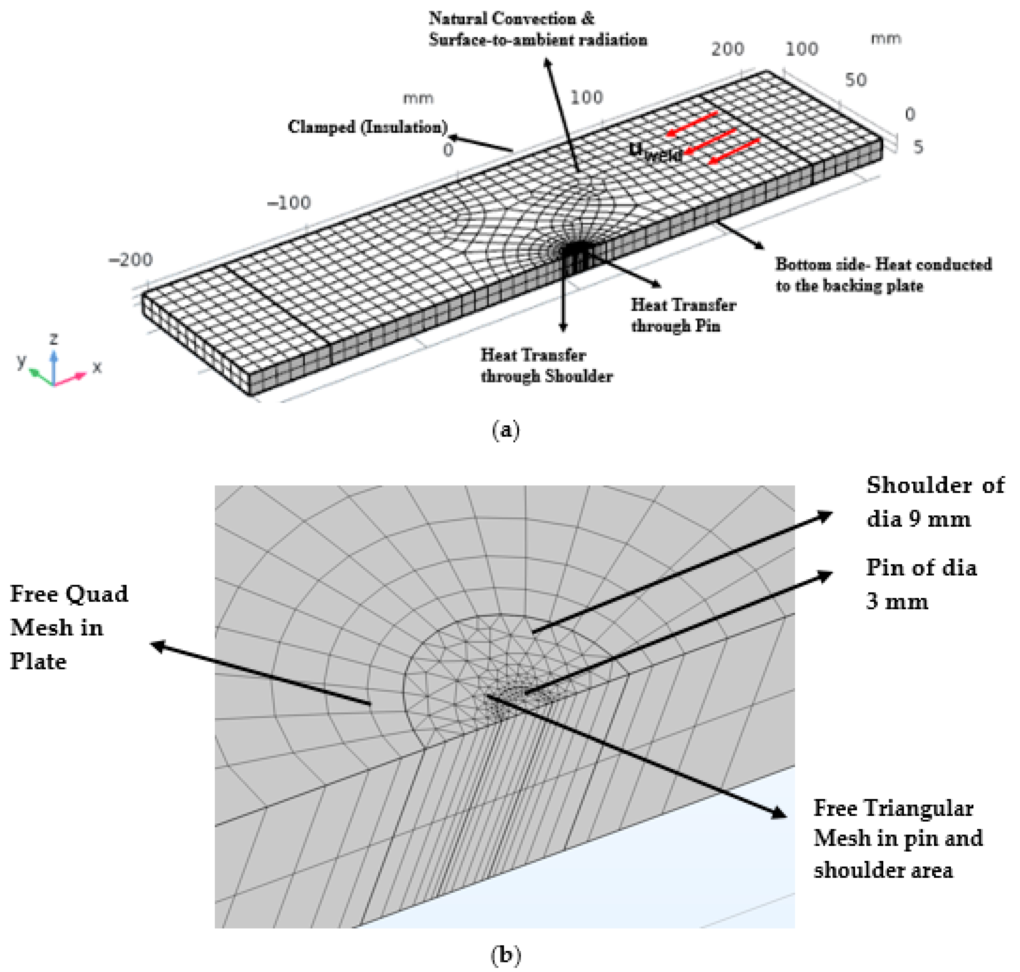
2.1. Modeling of FSW Plates in COMSOL

The dimensions of the Al 6061 T6 are a width of 120 mm, a length of 102 mm, and a thickness of 3 mm. Although two plates are needed to join the material using the FSW process, only one plate is sufficient to model due to the symmetry shown in Figure 1a. The material properties of Al 6061 T6 are listed in

Table 1. Material properties of Al 6061 T6 [32].

Temperature (K)	Density (kg/m3)	Specific Heat (cp) (J/kg K)	Thermal Conductivity, K (W/m K)
298	2700	896	180
311	2685	920	187
366	2685	978	194
422	2667	1004	201
477	2657	1028	206
533	2657	1052	214
589	2630	1078	220
644	2620	1104	227
700	2602	1133	233

. The FSW tool’s properties are imported from the built-in library of COMSOL 6.0; however, the tool geometry is modeled in the COMSOL modeler. The problem is defined as a stationary convection–conduction problem after making the coordinate transformation in which the tool remains plunged. At the same time, the aluminum 6061T6 plates are assumed to be infinitely long. During the FSW process, the joint is fabricated by the movement of the tool along the joint; however, this technique is complex when modeling the tool as a moving heat source. The modeling approach used in this work, in which the moving coordinate system is fixed to the tool axis, is also used by P. Chansoria et al., Song et al., and Zhu and Chao [29,30,31]. This makes the model much simpler to compute the maximum temperature.

The geometry is meshed using optimum mesh characteristics. The shoulder and pin area on top of the workpiece is meshed with a free triangular mesh with a fine size in COMSOL, while the remaining region of the workpiece is meshed with a free quad mesh (Figure 1b). The maximum and minimum sizes of the elements are set to 32 mm and 4.2 mm, respectively, with a curvature factor of 0.6 and a maximum growth rate of 1.45, ensuring accurate temperature prediction with maintained computational efficiency. The mesh is then extruded through the thickness of the workpiece.

2.2. Mathematical Models

The main sources of heat generation in FSW are shoulder–workpiece interaction and tool pin–workpiece interaction. The tool shoulder–workpiece interaction is due to friction and is modeled by Song et al. [30] using the following equation.

$$Q_s=2\pi \mu {\displaystyle \frac{F_n}{A_{shl}}}{R}_{shl}n$$

(1)

Many other investigations have also reported heat generation variations at the pin–workpiece interface [30,33]. However, few have considered it negligible, as reported by Zhu and Chao [31]. The heat generation and transfer processes are included in this work to model the FSW process accurately. Colegrove [34] provides the expression for the amount of heat from the pin, as shown in Equation (2).

$$Q_{pin}={\displaystyle \frac{2\pi \mu n}{\sqrt{3(1+{\mu }^2)}}}\overline{Y}{R}_{pin}\eta$$

(2)

The coefficient of friction is computed from the following equation reported by Arora et al. [35]. This equation is used in investigating the effect of the coefficient of friction on temperature, along with other parameters.

$$\mu ={\mu }_0\left(e^{\delta {\displaystyle \frac{nr}{n_0{R}_S}}}\right)$$

(3)

where

$$\delta =0.2+0.6\left(e^{{\delta }_0{\displaystyle \frac{nr}{n_0{R}_S}}}\right)$$

(4)

δ₀ is a constant value ranging between 0.2 and 0.8, depending upon the sticky or sliding condition. It is 0.3 in this analysis. n₀ is the reference rpm, taken as 300 rpm.

2.3. Governing Equations

P. Chansoria et al. [29] presented the following governing equations for modeling the FSW process as a transient heat transfer problem.

2.3.1. Heat Transfer Equation

The governing equation for the heat transfer problem is given as

$$\rho C_{p}u·\nabla \mathrm{T}=\nabla ·\left(k\nabla \mathrm{T}\right)+Q$$

(5)

This equation depicts the variation of temperature within Al 6061 T6 plates. The left-hand side of the equation represents the rate of change of energy in the material, while the right-hand side contains heat conduction and internal heat generation terms from friction and plastic deformation caused by the rotating tool.

2.3.2. Heat Loss from Upper Plate

The heat lost due to natural convection and surface-to-ambient radiation from the upper plate corresponds to the following heat flux equation.

$$e·\left(-k\nabla \mathrm{T}\right)=Q_{up}=h_{up}\left(T_0-\mathrm{T}\right)+\mathsf{\epsilon }\mathsf{\sigma }(T_0^2-T^4)$$

(6)

The term h_up (T₀ − T) represents the convective heat loss in ambient air, while the term εσ(T₀² − T⁴) accounts for radiative heat loss based on the Stefan–Boltzmann law.

2.3.3. Effect of Backing Plate

The backing plate is used in the FSW process and is placed below the plates to be joined together to maintain and contain the weld pool. The heat transfer through conduction at the backing plate is modeled as a convective heat transfer equation. Zhu and Chao [31] proposed heat flux equation:

$$e·\left(-k\nabla \mathrm{T}\right)=Q_{down}=h_{down}\left(T_0-\mathrm{T}\right)$$

(7)

The convective heat transfer coefficient at the bottom is higher than at the upper surface. Hence, the conduction heat transfer at the bottom is modeled as a convective heat transfer equation, assuming a fictitious convection coefficient approximately five times that of h_up. Zhu and Chao [31] use a similar assumption in their research.

2.3.4. Clamping of Plate

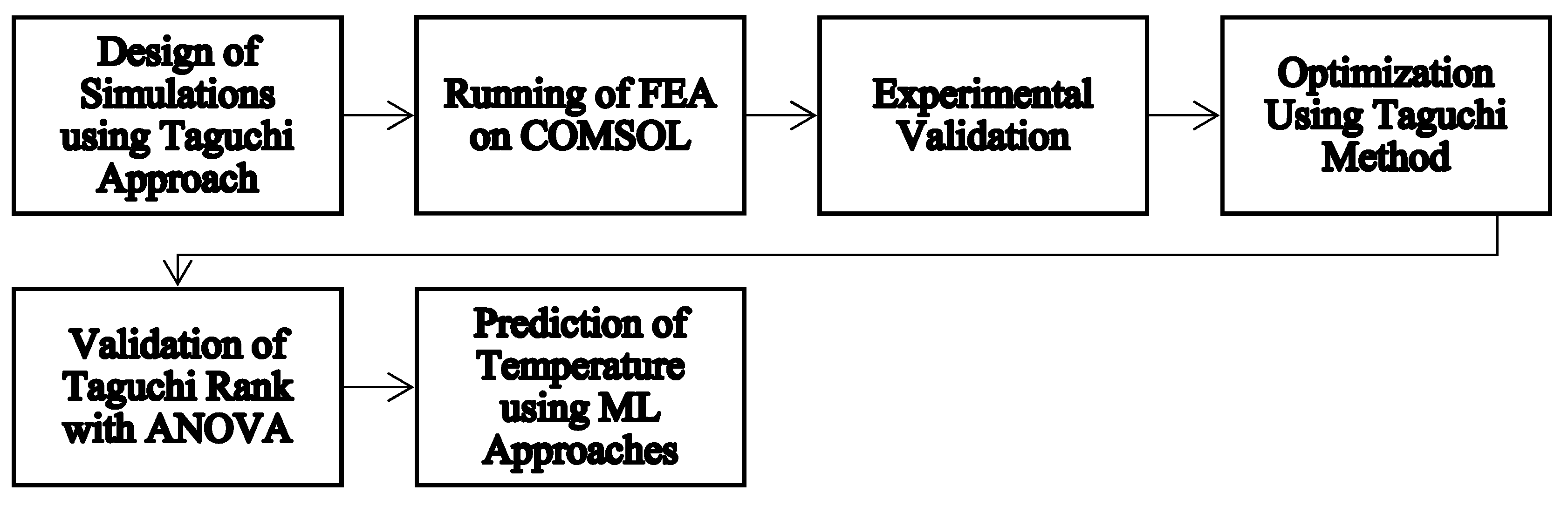
To restrict the movement of the workpiece and to ensure the proper weld formation, the plate is clamped at specified locations, as shown in Figure 1a. Due to thermal insulation conditions at clamped locations, Equation (7) can be rewritten as

$$e·\left(-k\nabla \mathrm{T}\right)=0$$

(8)

All governing equations (Equations (1)–(8)) were implemented using the Model Builder section interface in COMSOL Multiphysics. Equations (1) and (2), representing the frictional heat generated from shoulder–workpiece and pin–workpiece interaction, were implemented in the COMSOL Components section as Variable 1 and Variable 2, respectively. The coefficient of friction, dynamically calculated through Equations (3) and (4), was defined as a material-dependent variable under FSW parameters in COMSOL (

Table 2. FSW analysis parameters in COMSOL.

Parameters	Symbol	Value
Ambient temperature	To	300 [K]
Convection heat transfer coefficient on the top portion	hup	12.25 [W/m2 K]
Convection heat transfer coefficient on the bottom portion	hdown	61.25 [W/m2 K]
Surface emissivity	$\epsilon$ (epsilon)	0.3
Welding speed	u	Variable [mm/s]
Coefficient of friction	$\mu$	Variable
Rotational speed	$n$	Variable [rpm]
Angular velocity	${\omega }_o$	$2\pi n$ [rad/s]
Normal force (axial force)	Fn	Variable [kN]
Radius of pin	$R_{pin}$	Variable [mm]
Shoulder radius	$R_{shl}$	Variable [mm]
Shoulder surface area	$A_s$	$\pi (R_{shl}^2-R_{pin}^2)$
Mechanical efficiency (fraction of deformational work converted to heat)	$\eta$	0.9
Yield stress	$\overline{Y}$	[18]

). The governing heat transfer equation (Equation (5)) was applied through the Solids with Translational Motion feature to account for conduction and internal heat generation due to plastic deformation and friction. The convective and radiative heat losses from the top surface (Equation (6)) were incorporated using the Surface-to-Ambient Radiation and Heat Flux 1 boundary conditions. The heat transfer through the backing plate (Equation (7)) was modeled via Heat Flux 2, applying a fictitious convection coefficient. The thermal insulation at clamped boundaries (Equation (8)) was set by using a boundary heat source and insulation boundary conditions. These settings ensured accurate thermal modeling across all simulation domains and boundary conditions.

2.4. Process Flow

Figure 2 illustrates the process flow designed to investigate the effect of welding process parameters on peak temperature, followed by optimization and prediction through Taguchi, ANOVA, and ML classification. The design of simulations was the most crucial phase in this study and was used to select appropriate welding process parameters for the analyses. Several FEA simulations were conducted before adopting the L32 Taguchi array to explore thermal response across a wide range of welding parameters. Hence, these parameters were chosen based on preliminary simulation trials, the operational constraints of the milling machine, and a comprehensive previously published work [6,18,22,23], which identified them as having the most significant impact on the temperature distribution during FSW. The welding parameters analyzed in COMSOL were tool material, pin and shoulder diameter, tool rotational speed, welding speed, axial force, and coefficient of friction. The L32 Taguchi array was selected to efficiently optimize these parameters with a significantly reduced number of simulation runs compared to a full factorial design, which would require 2¹ × 4⁶ = 8192 runs. The levels of each process parameter are presented in

Table 3. Levels of FSW process parameters.

Factor	Level 1	Level 2	Level 3	Level 4
Pin Dia (mm)	3	4	5	6
Shoulder Dia (mm)	9	12	15	18
Tool Rotational Speed (rpm)	600	900	1200	1800
Welding Speed (mm/min)	20	38	50	80
Axial Force (kN)	1	5	8	10
Coefficient of Friction	0.3	0.33	0.36	0.40
Tool Material	H13	M2	--	--

. The Minitab 17 tool was used in this research to perform the Taguchi optimization and ANOVA.

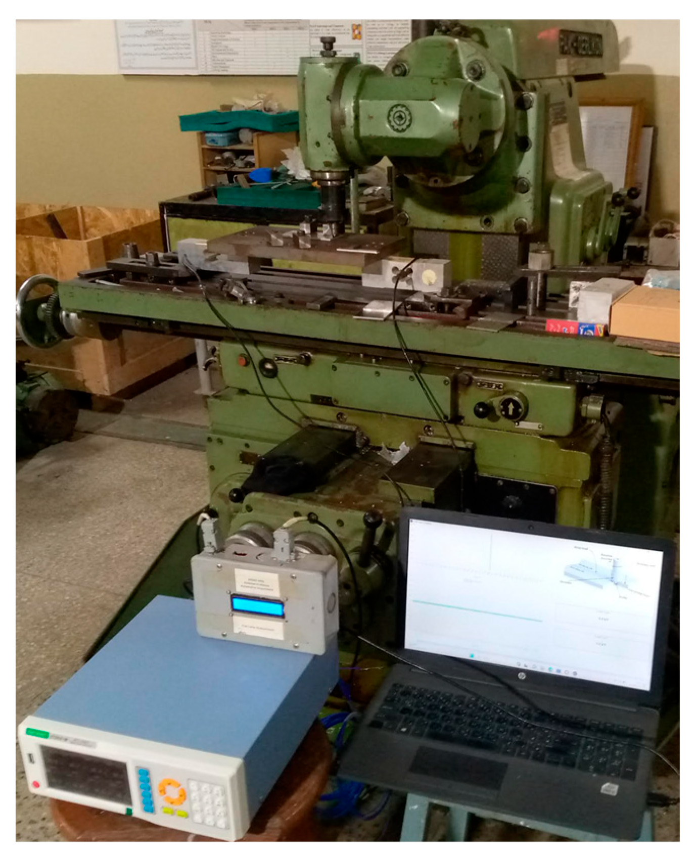
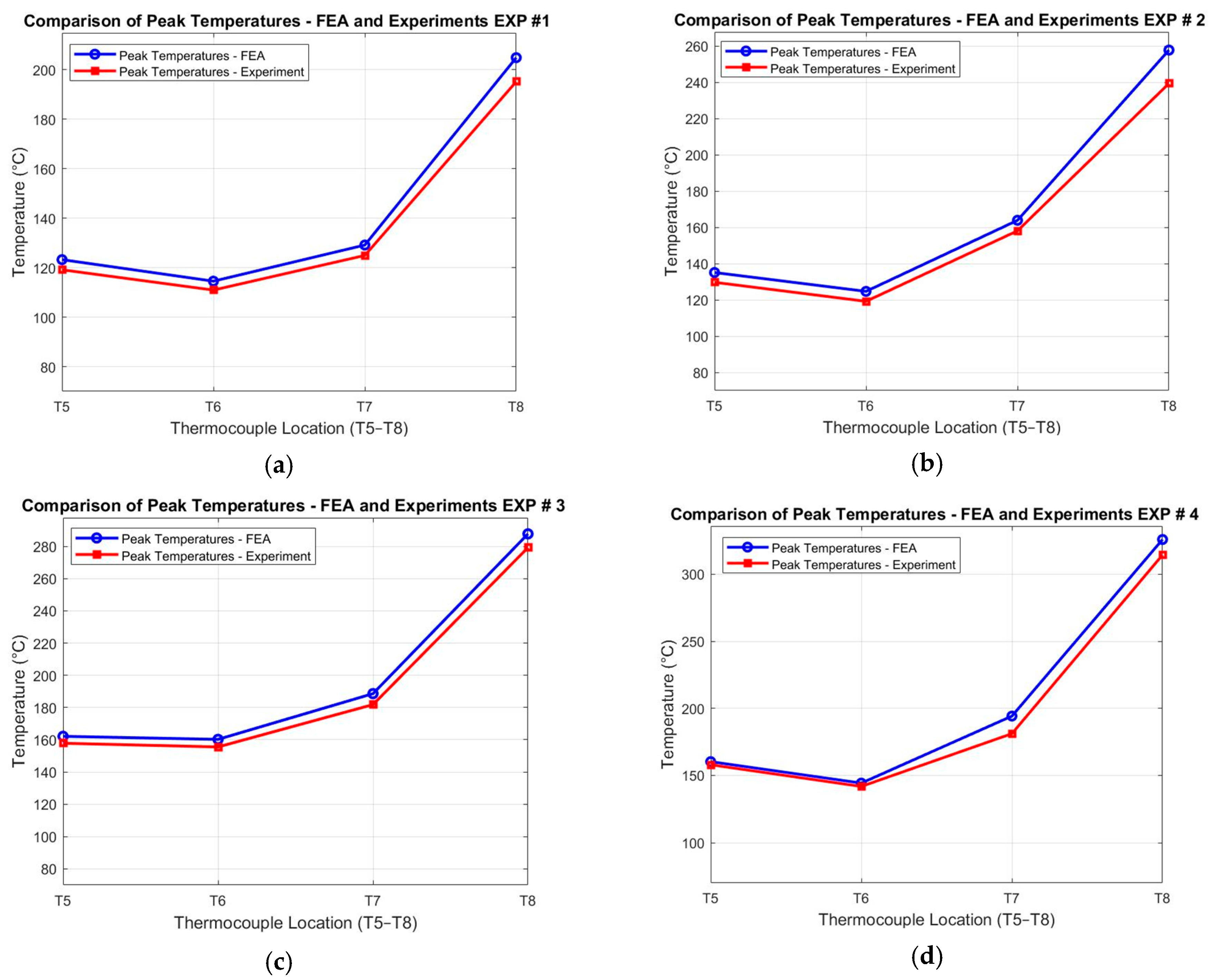
2.5. Experimental Details

A conventional universal milling machine was customized with a specially designed fixture and data acquisition system to conduct FSW experiments, as shown in Figure 3. A fixture was fabricated from a mild steel backing plate with a thickness of 23 mm to ensure rigidity during the FSW process. The fixture was designed to weld plates in butt joint configuration with a plate length not exceeding 200 mm. The plates were clamped through locally manufactured clamps and bolts to maintain a consistent joint during the welding operation. The axial force was measured using two compression-type load cells of 8 kN capacity. The load cells were attached just beneath the mild steel backing plate at both ends of the plate to measure the normal force during the FSW process. Arduino Uno-based software was developed to acquire force data during the welding process. The temperature was measured through K-type thermocouples, which were placed at eight different locations on the backing plate (Figure 4a,b). To ensure accurate peak temperature measurement without disturbing the weld surface, thermocouples were inserted through precisely drilled holes from the underside of the backing plate (Figure 4c). The sensor tips were tightly fitted to keep contact with the bottom surface of the welded plates, not the backing plate itself. This configuration minimized thermal lag and gradient effects, allowing reliable comparison with FEA-simulated temperature values at corresponding locations on the plate.

Thermocouples T8 and T4 were placed near the SZ in TMAZ, T3 and T7 near TMAZ in HAZ, T1 and T6 near HAZ, and T2 and T5 outside HAZ. The temperature data was captured through an ET3916-08 multichannel data logger at a sampling rate of 10 Hz. The Al 6061 T6 plates were cut to dimensions of 120 mm × 60 mm × 3 mm using a CNC machine and were cleaned with acetone before placement on the fixture. The welding operation was performed by four FSW tools made up of H13 steel with a hardness of 52 HRC, as shown in Figure 5. The experiments were conducted at a room temperature of 30 °C. Due to the operational limitations of the milling machine—which could operate at axial loads of 1–2 kN and rotational speeds of 480, 600, 670, 900, 1200, 1320, and 1800 rpm—the experiments were conducted using one axial load and four rotational speeds. The experimental parameters were selected from the Taguchi L32 array for the H13 tool material for an axial load of 1 kN. Due to equipment limitations, the experimental setup allowed welding only at an axial force of 1 kN. Consequently, the experimental trials were conducted solely at this level and used to validate the simulation model by comparing predicted and measured peak temperatures. Despite this constraint, the full factorial simulation design incorporated a broader range of axial forces (1, 5, 8, 10 kN), which enabled robust statistical and machine learning analysis. Therefore, while axial force was experimentally constant, its significance was evaluated comprehensively through a simulation-driven ANOVA. This constraint ensured that the experimental conditions were directly applicable to the available equipment while still allowing for a comprehensive investigation within the feasible parameter space.

3. Results and Discussion

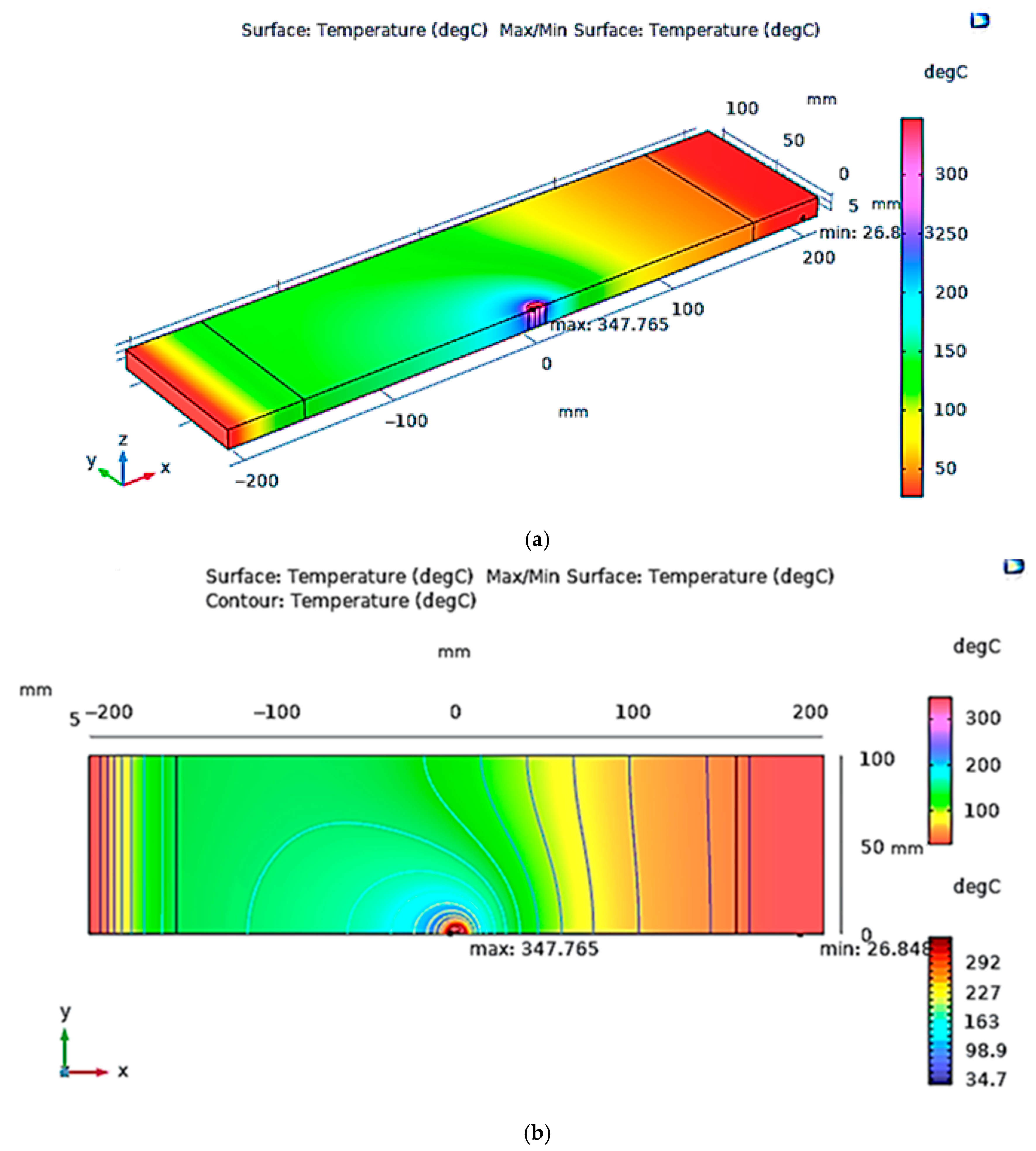
3.1. Temperature Distribution in Plates

The temperature distribution on the plate with a pin diameter of 3 mm, a shoulder diameter of 12 mm, axial force of 5 kN, a tool rotational speed of 900 rpm, transverse speed of 38 mm/min, and a coefficient of friction of 0.33 is shown in Figure 6a. The temperature distribution demonstrated a localized heat zone around the pin, extending outward along the shoulder contact area. The highest temperature attained in the weld region was 347.765 °C due to intense plastic deformation and frictional heat generation at the contact surface between the tool and the plate. Asmare et al. [36] in their experimental work reported this temperature to be 342 °C under similar assumed parameters; hence, this simulation analysis is in general agreement with previous published studies [23,36]. The top view of the temperature contour is shown in Figure 6b. It is evident from Figure 6b that the isotherms were closely packed in front of the tool axis than on the trailing side. This shows a rapid addition of heat at the weld zone and a slower heat loss rate on the trailing side.

The peak temperatures obtained from FEA simulations are listed in

Table 4. Peak temperatures obtained from COMSOL FEM simulations.

S No. #	Tool Material	Pin Dia (mm)	Shoulder Dia (mm)	Tool Rotational Speed (rpm)	Welding Speed (mm/min)	Axial Force (kN)	Coff. of Friction	Peak Temperature (°C)
1	H13	3	9	600	20	1	0.3	204.859
2	H13	3	12	900	38	5	0.33	347.765
3	H13	3	15	1200	50	8	0.36	659.193
4	H13	3	18	1800	80	10	0.4	677.67
5	H13	4	9	600	38	5	0.36	310.307
6	H13	4	12	900	20	1	0.4	257.821
7	H13	4	15	1200	80	10	0.3	658.577
8	H13	4	18	1800	50	8	0.33	668.699
9	H13	5	9	900	50	10	0.3	585.227
10	H13	5	12	600	80	8	0.33	358.117
11	H13	5	15	1800	20	5	0.36	659.917
12	H13	5	18	1200	38	1	0.4	287.83
13	H13	6	9	900	80	8	0.36	582.452
14	H13	6	12	600	50	10	0.4	555.809
15	H13	6	15	1800	38	1	0.3	325.941
16	H13	6	18	1200	20	5	0.33	645.24
17	M2	3	9	1800	20	10	0.33	679.418
18	M2	3	12	1200	38	8	0.3	529.137
19	M2	3	15	900	50	5	0.4	393.454
20	M2	3	18	600	80	1	0.36	174.855
21	M2	4	9	1800	38	8	0.4	660.469
22	M2	4	12	1200	20	10	0.36	660.224
23	M2	4	15	900	80	1	0.33	220.454
24	M2	4	18	600	50	5	0.3	269.265
25	M2	5	9	1200	50	1	0.33	273.268
26	M2	5	12	1800	80	5	0.3	549.489
27	M2	5	15	600	20	8	0.4	544.746
28	M2	5	18	900	38	10	0.36	659.703
29	M2	6	9	1200	80	5	0.4	568.452
30	M2	6	12	1800	50	1	0.36	342.561
31	M2	6	15	600	38	10	0.33	506.463
32	M2	6	18	900	20	8	0.3	658.856

. A large variation in peak temperature can be observed in the variation of selected process parameters. It is important to note that amongst other welding parameters, the tool rotational speed and axial force seem to be affecting the peak temperature in the FSW process. The higher rotational speed in combination with high axial force exhibited higher peak temperatures. This pattern showed a direct relationship between peak temperature and tool rotational speed and axial force. The highest temperature of 679 °C was achieved at a pin diameter of 3 mm, a shoulder diameter of 9 mm, a tool rotational speed of 1800 rpm, and axial force of 10 kN. The lowest temperature of 174 °C was obtained at the lowest levels of tool rotational speed and axial force, i.e., 600 rpm and 1 kN. Out of 32 simulations, the peak temperatures exceeded the threshold value of 600 °C on 11 occasions, as shown in Table 4. Though it was reported in several previously published research studies that peak critical temperature leads to precipitate coarsening, when the temperature exceeds the melting temperature, precipitate coarsening becomes a secondary issue, because the precipitate distribution is disrupted in the melted zone. The development of the precipitate-coarsening process cannot be ignored in the surrounding regions of the melting zone where the temperature reaches a critical value but remains below the melting point. It is crucial to note that this study focuses exclusively on predicting peak temperatures and identifying critical welding conditions during the FSW process of Al 6061 T6; thus, the effects of remelting or process resumptions are beyond the scope of this research. It is suggested that future research should address remelting strategies, including investigation of re-engagement speed and dwell time, thereby ensuring consistent weld quality.

The comparison of peak temperatures acquired from FEA simulations and experiments is presented in

Table 5. Comparison of experimental and FEA results.

Exp No.	Pin Dia (mm)	Shoulder Dia (mm)	Tool Rotational Speed (rpm)	Transverse Speed (mm/min)	Axial Force (kN)	Peak Temperature, FEA (°C)	Peak Experimental Temperature (°C)
1	3	9	600	20	1	204.85	195.10
2	4	12	900	20	1	257.82	239.40
3	5	18	1200	38	1	287.83	279.30
4	6	15	1800	38	1	325.94	314.40

. An error of less than 7% demonstrated close agreement between FEA and experiments, thus validating the computational model’s accuracy. Eight thermocouples (T1–T8) were placed on the Al 6061 T6 plate to measure temperatures on advancing and retreating sides; however, only four temperatures (T5–T8) were computed from FEA by placing a coordinate system in COMSOL. A comparison of COMSOL-analyzed and experimentally measured temperatures is presented in Figure 7a–d.

A comparative evaluation of peak temperature profiles at eight thermocouple locations for four distinctive experimental conditions is presented in Figure 8a–d. These figures reflect the relationship between tool geometry, tool rotational speed, and welding speed governing the heat generation, heat distribution, and heat dissipation dynamics during the FSW process. Importantly, the peak temperature is raised from 195 °C to 314 °C when the rotational speed is increased from 600 rpm (Exp # 1) to 1800 rpm (Exp # 4). This is due to high friction between the tool and the material caused by increased tool rotational speed, resulting in greater heat generation. Additionally, the time taken to reach the peak temperature is also reduced from 85 s (Exp # 1) to 55 s (Exp # 4), showing the generation of heat at higher speeds. This may improve material plasticization; however, it could also increase the risk of overheating and the grain growth process. Welding speed is another important parameter in understanding thermal behavior in FSW. Although the welding speed is nearly doubled from 20 to 38 mm/min in Exp # 3 as compared to Exp # 2, the increase in peak temperature is still observed from 239 °C to 279 °C. This reveals that while higher welding speeds tend to reduce heat input due to a shorter interaction time, the effect of increasing rotational speed on the temperature increase is more dominant than that of welding speed, likely due to a nonlinear relationship with frictional energy. Exp # 4 presents the combined effect of the highest levels of both speeds, resulting in the highest peak temperature of 314 °C. However, the reduced dwell time at the peak indicates a shorter thermal exposure at higher heating, leading to a condition that could favor a fine-grained microstructure with rapid cooling. The pin and shoulder diameters also influence the thermal behavior during welding by affecting the contact area and frictional heat generation. A larger pin diameter contributes to internal heat generation and appropriate material mixing by increasing the stirring volume beneath the surface; similarly, a larger shoulder diameter enhances frictional heat generation by increasing the contact area between the tool and the workpiece. This can be observed in Exp # 4, where the largest pin diameter of 6 mm and shoulder diameter of 15 mm in combination with high rotational and welding speed contribute to the highest heat input and rapid thermal response.

It is worth emphasizing that the temperature difference between the advancing and retreating sides (T8 and T4) in TMAZ revealed asymmetry in heat generation and material flow. At other locations, the temperature remained higher on the advancing side as compared with the retreating side, with minimal temperature difference. These patterns could be observed in all four temperature distribution plots. Keeping the asymmetric temperature distribution across advancing and retreating sides in mind, future studies should incorporate microstructural characterization to investigate material flow behavior and defects formation in weld zones.

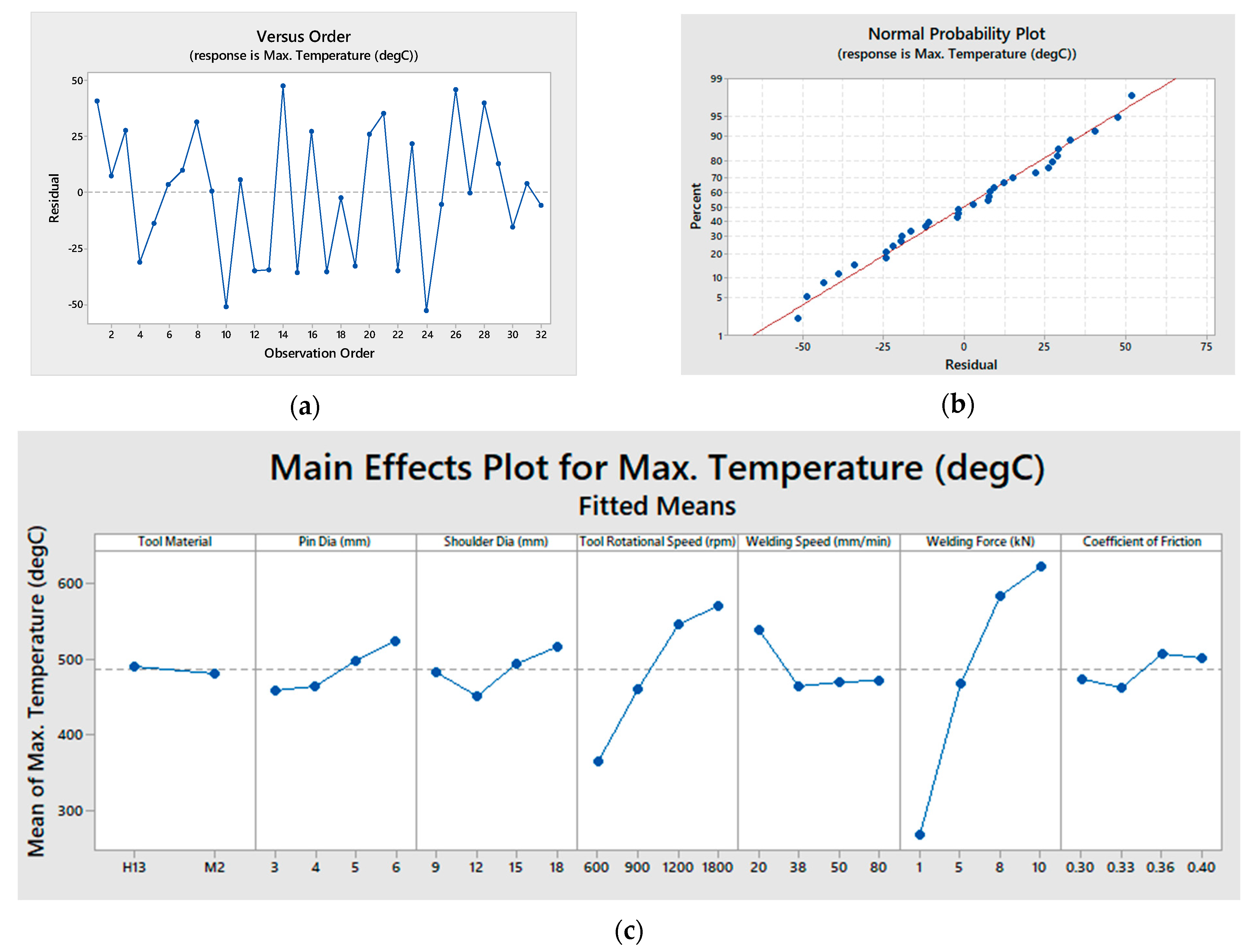
3.2. Taguchi Optimization

Taguchi’s optimization and analysis of variance (ANOVA) were used to optimize the process parameters to achieve the nominal temperature in the FSW welding process at a confidence level of 95%. This study aimed to optimize the FSW parameters to control the temperature, preventing it from exceeding the melting temperature, i.e., 600 °C, which is the critical threshold at which melting could occur in Al-6061-T6 alloys. The material’s structural integrity can be maintained further and poor-quality joints prevented by avoiding temperatures near the threshold. Hence, the “smaller is better” criterion was selected in the Taguchi method to minimize the maximum temperature. This approach was preferred over the “nominal is better” approach because it provides parameter combinations that yield lower maximum temperatures, ensuring control of overheating of the workpiece during FSW operation. This technique identifies the optimal settings that reduce peak temperatures, optimizing the process to remain within a safe range. The “smaller is better” criterion was utilized as it identifies settings that achieve low average values and maintain those values consistently. This is crucial for FSW processes to achieve a target value and minimize variability.

The rank and delta are two important indicators in Taguchi analysis. Rank represents the impact of each welding parameter on the response variable, while the delta value shows the difference between the highest and lowest S/N ratios calculated by the Taguchi method. The rank 1 and highest delta values signify each parameter’s sensitivity in the Taguchi method.

The response table was calculated from Equation (9) for signal-to-noise (S/N ratio), considering the “smaller is better” criterion, and it is tabulated in

Table 6. Response table for signal-to-noise ratio (using the “smaller is better” criterion).

Level	Tool Material	Pin Dia (mm)	Shoulder Dia (mm)	Tool Rotational Speed (rpm)	Welding Speed (mm/min)	Axial Force (kN)	Coff. of Friction
1	−53.1	−52.24	−52.95	−50.54	−53.90	−48.13	−52.81
2	−52.94	−52.40	−52.67	−52.65	−52.68	−52.96	−52.62
3		−53.33	−53.37	−54.10	−52.88	−55.15	−53.28
4		−54.11	−53.09	−54.79	−52.62	−55.84	−53.38
Delta	0.16	1.87	0.70	4.25	1.27	7.71	0.76
Rank	7	3	6	2	4	1	5

(while means are listed in

Table 7. Response table for mean values.

Level	Tool Material	Pin Dia (mm)	Shoulder Dia (mm)	Tool Rotational Speed (rpm)	Welding Speed (mm/min)	Axial Force (kN)	Coff. of Friction
1	486.6	458.3	483.1	365.6	538.9	260.9	472.7
2	480.7	463.2	450.1	463.2	453.5	468.0	462.4
3		489.8	496.1	535.2	468.4	582.7	506.2
4		523.2	505.3	570.5	473.8	622.9	493.3
Delta	5.9	64.9	55.1	205.0	85.4	361.9	43.7
Rank	7	4	5	2	3	1	6

). The higher negative values in the S/N table represent more stable and lower heat generation during FSW. Based on S/N ratios, mean values, rank, and delta values, it is evident from Table 6 and Table 7 that the axial force and tool rotational speeds are the most influential process parameters affecting peak temperature in FSW operations.

$${\displaystyle \frac{S}{N}}=-10{\log }_{10}\sum {\displaystyle \frac{Y^2}{n}}$$

(9)

where Y = the responses for the given factor level combination and n = the number of responses in the factor level combination.

3.3. Implementation of the ANOVA

An ANOVA was employed along with the Taguchi approach to validate and compare the ranking of FSW process parameters. The F-values and p-values are tabulated in

Table 8. ANOVA analysis.

Source	DF	Adj SS	Adj MS	F-Value	p-Value
Tool Material	1	280	280	0.12	0.731
Pin Dia (mm)	3	21,309	7103	3.16	0.064
Shoulder Dia (mm)	3	13,976	4659	2.07	0.158
Tool Rotational Speed (rpm)	3	196,580	65,527	29.11	0.000
Welding Speed (mm/min)	3	34,338	11,446	5.08	0.017
Axial Force (kN)	3	632,325	210,775	93.64	0.000
Coeff of Friction	3	9360	3120	1.39	0.294
Error	12	27,012	2251

. The p-values (<0.005) indicated that the axial force and the tool rotational speed significantly affected the FSW process. The higher F-values further revealed that axial force had the greatest effect on the process, followed by tool rotational speed, which is consistent with Taguchi’s results. The regression of the model is shown in Equation (10), and observation, normal probability, interaction, and main effect plots are shown in Figure 9a–c. Through residual analysis, the adequacy of the suggested regression models was tested. The observation order plots did not suggest any significant inadequacies in the model. The normal probability plot of residuals indicated that the residuals were approximately normally distributed. This suggested that the model adequately captured the variability in the maximum temperature data and supported the validity of the statistical analysis. A main effects plot revealed the influence of welding parameters on the maximum temperature. It was observed that the H13 resulted in a slightly lower maximum temperature than the M2 tool; however, the difference was minimal, showing the negligible impact of tool materials on maximum temperature. Pin diameter had a more moderate influence, with a gradual increase in maximum temperature as the diameter increased from 3 mm to 6 mm, likely due to a larger contact area and increased material deformation. Notably, tool rotational speed and welding force exhibited a clear and substantial impact on peak temperatures. The plot showed a strong positive correlation between rotational speed and maximum temperature, with temperatures rising dramatically as rotational speed increased from 600 rpm to 1800 rpm. Similarly, welding force demonstrated a pronounced effect, with maximum temperature increasing sharply as force increased from 1 kN to 10 kN. This relationship was attributed to the greater frictional resistance and plastic deformation occurring at higher forces, both of which contributed to heat generation.

The regression equation is as follows:

Max. Temperature (°C) = 483.63 + 2.96 Tool Material_H13 − 2.96 Tool Material_M2
−25.3 Pin Dia (mm)_3 − 20.4 Pin Dia (mm)_4 + 6.2 Pin Dia (mm)_5
+39.6 Pin Dia (mm)_6 − 0.6 Shoulder Dia (mm)_9
−33.5 Shoulder Dia (mm)_12 + 12.5 Shoulder Dia (mm)_15
+21.6 Shoulder Dia (mm)_18 − 118.1 Tool Rotational Speed (rpm)_600
−20.4 Tool Rotational Speed (rpm)_900
+51.6 Tool Rotational Speed (rpm)_1200
+86.9 Tool Rotational Speed (rpm)_1800
+55.3 Welding Speed (mm/min)_20 − 30.2 Welding Speed (mm/min)_38
−15.2 Welding Speed (mm/min)_50 − 9.9 Welding Speed (mm/min)_80
−222.7 Axial Force (kN)_1 − 15.6 Axial Force (kN)_5
+99.1 Axial Force (kN)_8 + 139.3 Axial Force (kN)_10
−11.0 Coefficient of Friction_0.30
−21.2 Coefficient of Friction_0.33
+22.5 Coefficient of Friction_0.36
+9.6 Coefficient of Friction_0.40

(10)

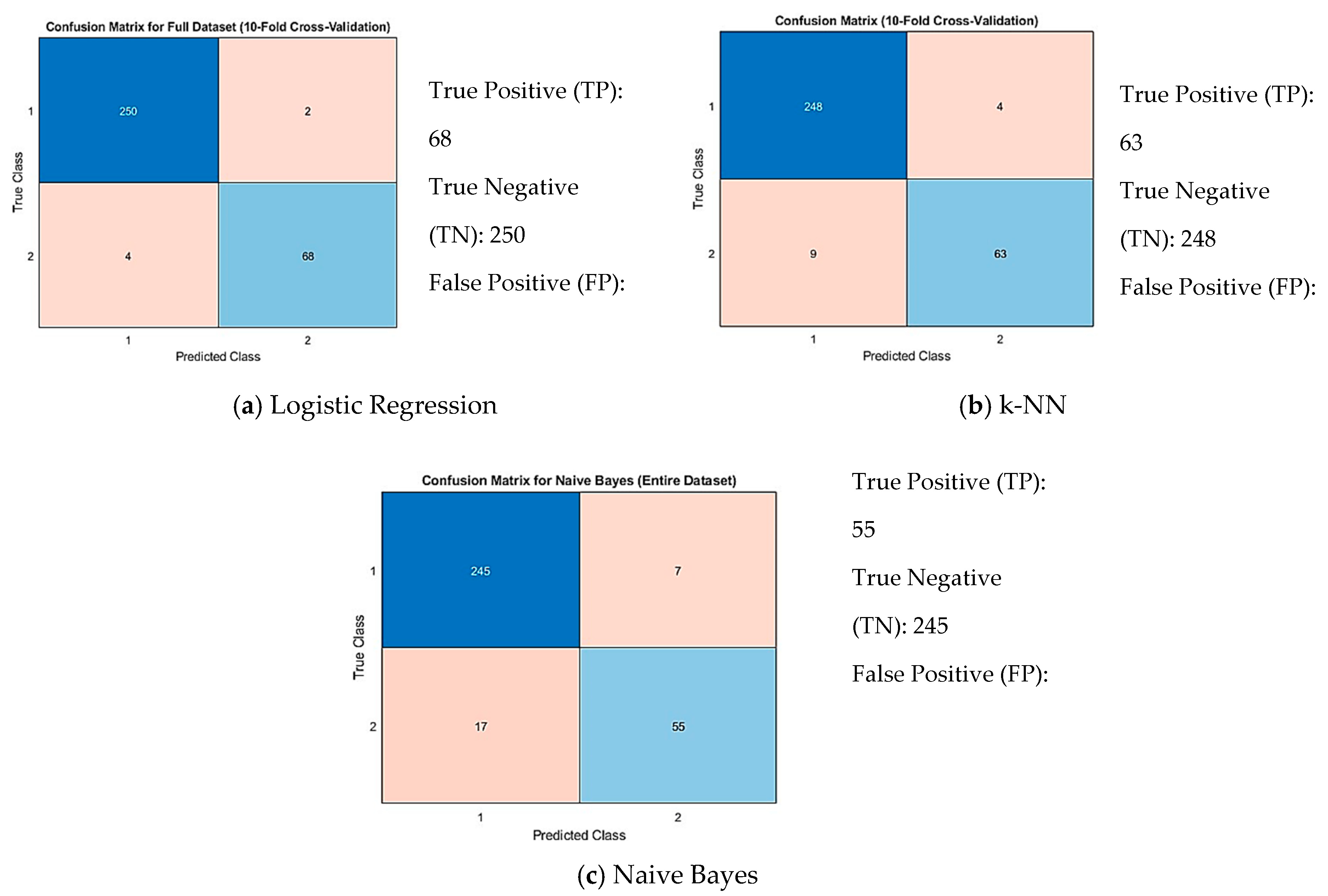
3.4. ML Classification Approaches

The selection of input variables to implement ML classifiers was carried out through ANOVA analysis. Table 8 reveals that all parameters investigated in the study were significant except for tool material, shoulder diameter, and coefficient of friction, with a p-value greater than 0.05. Hence, for the implementation of a machine learning-based classification model, these parameters were not considered. Although shoulder diameter was found to be statistically insignificant in the ANOVA analysis, it was included in the COMSOL simulations for geometric consistency. Specifically, the tools were designed and fabricated based on a pin-to-shoulder diameter ratio of 1:3, which necessitated defining the shoulder diameter for each corresponding pin diameter in the simulations. Therefore, shoulder diameter was indirectly represented in the thermal simulations, but it was not treated as a separate variable in the machine learning classification due to its statistical insignificance.

Considering the large dataset requirement of the ML models, a new dataset of 324 datapoints was prepared through factorial design. A factorial design (3⁴ × 4¹) containing 4 parameters of 3 levels and 1 parameter of 4 levels resulted in a simulation set of size 324 for performing FEA in COMSOL Multiphysics; a total of 324 independent simulations were carried out to achieve transient temperatures. The levels of the parameters are presented in

Table 9. Factorial design of selected parameters.

Factor	Level 1	Level 2	Level 3	Level 4
Pin Dia (mm)	4	5	6	---
Shoulder Dia (mm)	12	15	18	---
Tool Rotational Speed (rpm)	670	950	1320	---
Welding Speed (mm/min)	20	45	85	---
Axial Force (kN)	1	3	5	9
Tool Material	H13 Tool Steel

, and the peak temperatures from the COMSOL simulations are provided in Appendix A (

Table A1. Dataset Obtained from COMSOL 6.0 FEM Simulations.

S. No	Pin Dia	Shoulder Dia	Tool Rotational Speed	Welding Speed	Axial Force	Transient Temperature
1	5	15	1320	45	1	292.818
2	5	15	950	45	1	264.1
3	4	12	950	85	5	386.242
4	4	15	670	20	5	394.013
5	4	12	1320	45	1	272.048
6	4	18	950	20	3	378.807
7	4	12	1320	45	3	392.547
8	5	18	1320	85	5	539.81
9	4	18	950	45	8	659.231
10	5	18	670	85	5	325.289
11	4	15	950	20	3	365.481
12	5	12	1320	20	5	659.375
13	6	15	950	45	8	659.585
14	6	18	670	85	5	342.688
15	4	15	670	85	8	413.094
16	5	12	1320	20	3	479.977
17	5	15	950	85	8	585.875
18	6	15	1320	45	5	658.771
19	6	18	1320	20	5	660.333
20	6	18	950	45	3	369.446
21	4	12	670	20	3	296.422
22	5	15	1320	85	8	659.744
23	5	15	1320	20	1	316.519
24	5	15	670	45	1	243.544
25	5	12	1320	85	1	281.011
26	6	18	1320	85	3	401.116
27	4	18	1320	20	1	293.268
28	4	18	1320	20	3	492.424
29	6	12	670	85	8	466.992
30	4	12	950	20	3	356.779
31	5	18	950	20	3	399.155
32	4	18	670	45	1	223.778
33	6	12	1320	85	5	574.604
34	5	12	670	85	1	233.754
35	6	15	670	20	3	341.087
36	6	12	950	20	1	303.703
37	6	18	670	20	8	658.742
38	6	18	950	85	3	334.315
39	6	12	670	20	1	270.615
40	5	15	670	45	3	291.801
41	6	18	670	85	8	458.704
42	4	15	1320	20	1	289.975
43	5	15	1320	20	5	659.488
44	4	18	950	45	1	247.73
45	5	12	1320	45	3	424.1
46	6	18	950	85	1	266.384
47	5	18	950	85	8	600.957
48	4	18	1320	45	1	269.7
49	6	12	670	45	5	386.693
50	6	15	670	45	1	257.594
51	4	15	670	20	8	576.149
52	6	15	670	85	5	346.576
53	4	12	1320	85	3	357.716
54	4	15	950	45	1	247.879
55	6	12	950	45	3	322.545
56	4	18	1320	85	8	659.736
57	6	15	1320	20	3	463.688
58	5	15	950	45	8	659.199
59	6	12	670	45	8	522.931
60	6	18	670	20	3	344.028
61	4	15	670	85	3	253.939
62	4	12	670	45	3	273.461
63	5	18	950	85	5	411.647
64	4	12	1320	85	1	260.299
65	4	12	950	20	1	261.205
66	6	18	950	85	5	432.147
67	4	15	1320	45	5	592.014
68	6	15	1320	85	3	405.928
69	4	12	1320	20	8	660.214
70	5	18	1320	20	1	317.835
71	6	12	950	85	3	347.379
72	5	15	1320	45	5	627.364
73	6	15	950	20	5	593.034
74	6	15	950	20	8	659.976
75	6	12	950	45	8	659.632
76	5	15	1320	20	8	661.123
77	4	18	950	85	1	235.239
78	5	15	950	85	1	254.247
79	5	12	950	45	3	347.59
80	4	15	1320	20	8	660.931
81	5	12	670	85	5	333.912
82	6	15	670	20	5	438.032
83	4	18	670	20	3	304.853
84	5	12	950	85	8	583.25
85	5	15	950	45	3	346.186
86	5	12	1320	45	5	607.639
87	4	15	1320	20	5	659.257
88	6	12	1320	45	5	655.283
89	6	12	1320	85	1	301.315
90	4	18	1320	45	5	624.77
91	6	12	1320	85	8	660.282
92	5	15	950	20	3	388.187
93	5	12	950	20	1	280.751
94	5	15	670	85	8	434.039
95	6	12	670	20	3	341.785
96	5	12	1320	20	8	660.509
97	6	18	670	45	8	545.751
98	6	12	670	85	3	298.136
99	6	15	670	45	8	527.343
100	4	12	670	85	1	212.511
101	5	18	1320	20	8	661.346
102	6	12	1320	20	1	341.735
103	5	12	950	85	5	413.368
104	5	18	1320	45	8	666.28
105	5	12	950	20	8	659.68
106	6	12	950	85	1	272.391
107	4	12	670	85	3	256.74
108	4	12	1320	85	8	659.498
109	6	12	670	85	5	357.356
110	5	15	670	85	3	272.636
111	5	18	1320	85	8	659.813
112	6	15	950	85	8	618.321
113	4	12	670	45	8	460.784
114	6	18	1320	85	8	660.373
115	6	12	950	45	1	284.199
116	5	12	950	20	5	529.689
117	6	12	670	45	1	259.458
118	6	18	670	45	5	386.008
119	4	15	670	85	5	307.758
120	4	18	670	20	1	239.002
121	6	18	950	20	5	620.185
122	4	15	670	20	1	238.341
123	5	12	1320	45	8	660.81
124	4	18	950	85	8	578.271
125	6	15	670	45	5	383.145
126	5	18	670	20	5	432.07
127	5	12	950	45	8	658.901
128	5	18	670	85	3	270.116
129	4	15	950	20	1	260.672
130	5	15	950	85	5	418.712
131	6	18	1320	20	8	661.485
132	6	18	1320	20	1	340.176
133	5	12	950	85	3	324.037
134	6	12	1320	20	8	673.359
135	5	12	670	45	1	244.762
136	4	12	950	85	1	237.408
137	5	12	670	20	8	572.431
138	6	15	950	20	1	302.608
139	5	18	1320	85	1	273.705
140	4	15	670	45	5	341.266
141	5	12	1320	85	3	386.198
142	5	15	1320	85	5	530.211
143	6	15	1320	85	1	297.056
144	6	12	950	20	3	412.583
145	4	15	950	85	5	386.272
146	4	15	670	45	8	478.643
147	5	12	670	20	1	256.415
148	5	15	670	20	5	414.613
149	5	15	670	20	1	255.507
150	5	12	670	45	3	295.295
151	6	15	950	20	3	414.508
152	6	12	950	85	8	625.06
153	6	12	670	45	3	315.11
154	6	12	670	20	5	431.979
155	6	15	670	85	1	248.203
156	5	18	1320	45	3	432.244
157	5	18	950	20	5	588.731
158	4	18	1320	85	3	357.402
159	6	18	950	20	3	423.268
160	4	18	670	85	5	309.079
161	6	18	1320	45	1	315.105
162	6	18	950	45	1	280.207
163	6	15	670	20	8	635.289
164	6	18	950	20	1	303.04
165	5	12	670	45	8	489.421
166	4	12	950	45	5	429.714
167	5	15	670	20	3	319.667
168	5	18	950	85	3	314.025
169	6	15	1320	20	1	339.517
170	5	15	1320	85	3	379.556
171	6	15	1320	20	8	661.913
172	5	18	670	20	8	639.006
173	4	12	950	45	8	630.716
174	5	12	670	20	5	404.608
175	5	15	670	20	8	603.143
176	4	15	1320	85	3	354.456
177	5	15	950	45	5	465.658
178	5	18	1320	20	5	659.634
179	4	12	950	85	3	300.504
180	5	18	950	20	1	280.419
181	4	18	670	85	3	252.997
182	5	12	1320	85	5	531.863
183	4	12	1320	45	8	660.301
184	4	12	670	85	5	310.599
185	6	18	1320	20	3	562.547
186	5	18	1320	85	3	378.661
187	6	12	950	85	5	445.463
188	4	15	1320	45	1	270.199
189	4	18	950	85	5	393.108
190	5	18	670	45	3	291.351
191	6	15	1320	45	1	316.14
192	4	15	950	45	8	658.301
193	6	18	1320	45	8	661.268
194	6	18	670	85	1	247.05
195	4	18	1320	20	5	659.513
196	5	12	670	45	5	361.008
197	4	12	1320	20	3	444.476
198	5	18	670	20	1	255.399
199	5	12	950	85	1	256.482
200	6	15	670	45	3	310.019
201	5	12	1320	45	1	294.821
202	6	15	950	45	5	493.584
203	4	12	1320	45	5	565.355
204	6	15	670	85	8	457.317
205	4	15	950	85	8	558.211
206	4	18	950	20	1	261.028
207	5	18	950	45	8	659.412
208	4	15	1320	85	5	501.443
209	6	15	670	85	3	290.748
210	5	12	950	20	3	383.803
211	6	18	1320	85	5	569.763
212	5	15	670	85	5	327.086
213	6	12	950	20	8	659.952
214	6	12	670	20	8	612.025
215	4	15	950	45	5	441.186
216	6	18	670	20	5	452.63
217	4	18	670	85	8	423.258
218	4	15	950	20	5	526.294
219	6	18	950	85	8	628.289
220	5	15	1320	20	3	497.149
221	5	18	670	45	5	368.077
222	4	18	1320	45	8	660.429
223	4	18	1320	20	8	668.412
224	5	12	950	45	5	459.279
225	4	15	950	20	8	659.671
226	4	12	670	20	1	238.335
227	4	18	950	85	3	294.206
228	4	12	670	85	8	409.463
229	6	15	1320	45	3	454.659
230	6	15	950	85	3	338.244
231	4	15	950	85	1	235.9
232	5	15	950	20	8	660.217
233	4	18	670	45	8	503.201
234	6	18	1320	45	5	659.168
235	4	18	950	20	5	562.5
236	4	15	670	20	3	298.397
237	5	18	950	45	1	263.197
238	6	15	1320	85	8	660.004
239	6	18	670	20	1	268.63
240	4	12	950	20	8	659.44
241	4	18	670	45	5	351.118
242	4	18	670	20	8	616.466
243	4	12	950	85	8	546.594
244	6	15	1320	85	5	564.397
245	5	12	1320	85	8	659.762
246	6	18	670	45	1	256.686
247	4	18	1320	85	1	256.972
248	6	15	1320	45	8	661.012
249	6	18	670	45	3	309.203
250	5	18	950	45	5	480.662
251	5	15	950	20	1	279.666
252	6	15	950	45	3	369.521
253	5	18	950	20	8	663.023
254	4	12	1320	20	5	658.853
255	6	15	1320	20	5	659.78
256	4	15	1320	85	1	258.077
257	5	18	1320	20	3	523.272
258	4	12	1320	85	5	495.184
259	6	12	950	45	5	493.49
260	6	18	1320	85	1	294.85
261	5	18	670	85	1	231.443
262	5	12	950	45	1	266.37
263	5	12	670	85	8	436.211
264	4	18	950	20	8	659.801
265	6	15	670	20	1	269.212
266	4	15	950	45	3	321.854
267	5	18	950	45	3	348.319
268	5	18	670	85	8	439.735
269	6	15	950	85	5	433.973
270	4	18	670	85	1	210.794
271	5	12	670	85	3	277.828
272	5	15	950	20	5	556.827
273	4	15	1320	45	8	659.966
274	4	12	670	20	5	379.14
275	4	18	1320	45	3	409.336
276	4	18	670	20	5	414.603
277	5	18	670	45	1	243.11
278	4	12	950	45	3	322.545
279	4	15	1320	45	3	397.964
280	5	15	1320	45	8	661.692
281	4	12	670	45	1	224.087
282	6	18	950	45	5	506.02
283	4	12	950	20	5	495.285
284	4	15	670	45	3	272.24
285	4	15	670	85	1	211.323
286	6	12	1320	85	3	418.386
287	5	18	1320	45	1	292.745
288	5	18	1320	45	5	654.997
289	4	15	1320	85	8	659.62
290	6	18	950	45	8	659.562
291	5	15	670	45	8	500.942
292	5	18	950	85	1	253.043
293	6	12	1320	45	1	319.199
294	4	18	950	45	3	327.388
295	4	18	950	45	5	460.245
296	5	15	1320	85	1	275.743
297	4	15	1320	20	3	463.688
298	4	18	1320	85	5	515.518
299	4	18	670	45	3	273.386
300	6	12	1320	20	3	523.121
301	6	12	1320	20	5	660.75
302	4	15	670	45	1	223.613
303	5	15	1320	45	3	423.877
304	6	12	1320	45	8	660.261
305	5	12	1320	20	1	316.857
306	6	18	1320	45	3	459.276
307	4	12	670	45	5	337.992
308	5	15	950	85	3	316.986
309	5	15	670	85	1	232.214
310	4	12	1320	20	1	289.45
311	5	18	670	20	3	324.975
312	4	12	670	20	8	538.335
313	6	12	950	20	5	573.128
314	5	12	670	20	3	317.596
315	6	12	1320	45	3	458.121
316	6	18	950	20	8	659.961
317	6	15	950	45	1	281.306
318	4	12	950	45	1	248.896
319	6	12	670	85	1	250.301
320	6	18	670	85	3	286.851
321	4	15	950	85	3	295.739
322	6	15	950	85	1	268.773
323	5	18	670	45	8	522.429
324	5	15	670	45	5	361.759

).

The dataset was projected through three ML classification models, i.e., Logistic Regression, k-Nearest Neighbor, and Naive Bayes. In solid-state welding, the material’s temperature remains below its melting point. For Al 6061-T6, a melting temperature of 600 °C was used to categorize the dataset. Kishan et. al. [26], Mishra and Morisetty [37], and Thapliyal and Mishra [25] adopted a similar approach in their research, classifying tensile strength based on a joint efficiency criterion of more than 70%. However, this study employed the peak temperature criterion, ensuring that it did not exceed the material’s melting point, as the basis for categorization. The response variable was binary, indicating whether the temperature exceeded 600 °C. The classification assigned a value of 0 to outputs where the temperature fell below 600 °C and 1 to those where the temperature exceeded 600 °C. Logistic Regression is an ML classification statistical method that uses a sigmoid function to map input features to a probability between 0 and 1, making it ideal for determining whether the temperature is above or below a threshold value.

In this study, the Logistic Regression was employed to classify the temperature as either class 1, where temperature > 600 °C, or class 0, where temperature ≤ 600 °C. k-NN is a distance-based, instance-based learning algorithm. The “k” in k-NN indicates the number of neighbors used to classify a new data point. In the k-NN algorithm, the k closest points from the training set are considered for each data point in the testing set. The algorithm assigns the majority class among these neighbors to the testing point. In this analysis, k = 1 yielded optimal results. Naive Bayes is a probabilistic classifier based on Bayes’ theorem. It assumes conditional independence among features, enabling simplified computation by evaluating feature likelihoods independently. It classifies data as 0 or 1 by calculating the posterior probabilities for each class using Bayes’ theorem and assigning the class with higher probability.

3.5. Implementation of ML Classification Models

After the dataset preparation, ML models were employed to train and test the dataset. These models were trained using the K-fold cross-validation technique to assess their robustness across different subsets of data. Cross-validation is a technique extensively used in ML algorithms to avoid overfitting, especially in scenarios with small datasets. This method divides the fixed portion of a dataset for validation and the remaining portion for training a model. The process is reiterated after testing, with a different portion of data allocated as the validating set. The “K” in cross-validation is the split count for the validation and training datasets. A 10-fold cross-validation was implemented in this work, where the model was trained on 90% of the data in each fold and validated on the remaining 10%; this process was repeated ten times. The ML classification models were compared through five model evaluation metrics: accuracy, F1 score, precision, recall, and error. These metrics were calculated using Equations (11)–(15) and are presented in

Table 10. Evaluation metrics of classifier models.

Classifier Model	Accuracy	F1 Score	Precision	Recall	Error
Logistic Regression	0.9814	0.9577	0.9714	0.9444	0.0180
k-NN	0.9598	0.9064	0.9402	0.8750	0.0401
Naive Bayes	0.9259	0.8208	0.8870	0.7638	0.0740

. TP indicates true positive, TN is true negative, FP is false positive, and FN represents false negative. The highest accuracy was achieved with the Logistic Regression ML classifier, indicating that 98.14% of all predictions were correct, suggesting higher overall performance in binary classification. The F1 score balances precision and recall. A higher F1 score suggests that the ML algorithm is reasonably good at predicting temperatures > 600 °C without too many false negatives or positives. The accuracy of positive predictions is reflected by precision, whereas recall measures how well the model identifies all true positives. Table 10 depicts that the Logistic Regression ML classifier showed the best performance among all evaluated ML classifiers, achieving the highest accuracy, F1 score, recall, and precision. Further, its accuracy of 98.14% is also the highest reported in the published literature. In comparison, Thapliyal and Mishra [25] reported an accuracy of 94% using an Artificial Neural Network (ANN), while Kishan et. al. [26] achieved an accuracy of 81.6% utilizing the Adaptive Boosting classifier. The confusion matrices for all three ML classifiers are shown in Figure 10.

Accuracy = (TP + TN)/N

(11)

F1 Score = [(Precision × Recall)/(Precision + Recall)] × 2

(12)

Precision = TP/(TP + FP)

(13)

Recall = TP/(TP + FN)

(14)

Error = (FP + FN)/N

(15)

To further evaluate the performance of the classification models, ROC curves (Figure 11) were generated, and the corresponding AUC values were calculated. The AUC values obtained were 0.99757 for Logistic Regression, 0.98677 for k-NN, and 0.98319 for Naive Bayes. These values indicate a high degree of separability and excellent classification capability for all models. Logistic Regression demonstrated the best overall performance, not only achieving the highest classification accuracy of 98.14% but also the highest AUC, confirming its superior ability to distinguish between classes. Although k-NN and Naive Bayes yielded slightly lower AUCs, they still maintained strong classification potential, with k-NN exhibiting good precision and Naive Bayes offering effective probabilistic separation. The ROC curves complement traditional performance metrics and validate the robustness of the classifiers in predicting thermal thresholds in FSW simulations.

4. Industrial Applications

The findings of this study have significant potential for industries that depend on advanced manufacturing processes, particularly additive manufacturing and FSW operations. In the aerospace industry, where highly efficient materials and defect-free joints are critical, the ML modeling approach can facilitate reliable and efficient processes. By accurately forecasting temperature profiles and optimizing welding parameters, manufacturers can reduce defects, improve mechanical properties, and improve the quality of aerospace components.

Furthermore, this research can be applied to other high-precision manufacturing industries, such as automotive and defense, in which strong lightweight materials are in high demand. The incorporation of machine learning models into manufacturing workflows results in real-time process control, thus minimizing experimental costs and material wastage. As industries shift towards Industry 4.0 and smart manufacturing, the adoption of artificially intelligent predictive models like the one proposed in this research has tremendous potential for application in process automation, quality assurance, and performance optimization of various engineering applications.

5. Conclusions

This paper presents the application of the Taguchi method, ANOVA, and ML classification approach to control and predict peak temperatures in FSW of Al-6061-T6 aluminum alloys. The “smaller is better” criterion was employed in Taguchi analysis to keep the temperatures below the melting point, preventing overheating during FSW operation. An ANOVA was used to rank the process parameters, and it was found that axial force and tool rotational speed are the most significant parameters affecting peak temperatures. However, the coefficient was found to have an insignificant effect on temperature, as revealed by Taguchi and the ANOVA. Taguchi and ANOVA ranks were in good agreement, providing valuable insights into the parameter hierarchy, enabling targeted adjustments to improve weld quality effectively. The dataset of 324 datapoints was subsequently classified using three ML algorithms: Logistic Regression, k-NN, and Naive Bayes. Based on ML performance metrics (i.e., accuracy, F1 score, precision, recall, and error), it was found that Logistic Regression demonstrated the best performance, achieving an accuracy of 98.14%, which is among the highest in the FSW domain.

The findings herein are significant for sustainable manufacturing, as precise predictions of peak temperatures in FSW can minimize energy consumption and material waste while optimizing process parameters. This approach contributes to reducing experimental costs and carbon footprints associated with traditional trial-and-error methods in manufacturing. By leveraging advanced computational techniques, this research aligns with global efforts to promote sustainable manufacturing practices through intelligent process optimization.

This research work has primarily focused on optimizing and predicting peak temperature during the FSW process using FEA simulations, Taguchi, an ANOVA, and an ML classification approach. Experimental validations were performed under milling machine constraints, where the axial force was kept constant. The effect of pin profiles and shoulder shapes, high dynamic axial force, and remelting behavior was beyond the scope of this study. Future studies should incorporate tool geometrical features, varied axial force, microstructural analysis, defect characterization, and remelting procedure to establish a strong correlation between thermal behavior and joint quality. Additionally, future studies could expand this comparative approach to other alloys, adding experimental validations and exploring additional machine learning algorithms to enhance the model’s robustness for broader industrial applications, particularly in sustainable manufacturing.

References

1. Thomas, W.M.; Nicholas, E.D.; Needham, J.C.; Murch, M.G.; Temple-Smith, P.; Dawes, C.J. Friction Stir Butt Welding, International Patent Application PCT/GB92/02203, GB Patent Application 9125978.8, US Patent 5.460.317. Available online: https://www.mendeley.com/catalogue/d39ca923-225d-3e7c-8bc9-7ccca2e23b99/?utm_source=desktop&utm_medium=1.19.8&utm_campaign=open_catalog&userDocumentId=%7B01c2fd14-2fc6-391f-8c00-6ed88f2dca45%7D (accessed on 17 March 2025).
2. Kumar, S.S.; Murugan, N.; Ramachandran, K.K. Effect of tool tilt angle on weld joint properties of friction stir welded AISI 316L stainless steel sheets. Measurement 2020, 150, 107083. [Google Scholar] [CrossRef]
3. Zhang, S.; Shi, Q.; Liu, Q.; Xie, R.; Zhang, G.; Chen, G. Effects of tool tilt angle on the in-process heat transfer and mass transfer during friction stir welding. Int. J. Heat Mass Transf. 2018, 125, 32–42. [Google Scholar] [CrossRef]
4. Shankar, S.; Vilaça, P.; Dash, P.; Chattopadhyaya, S.; Hloch, S. Joint strength evaluation of friction stir welded Al-Cu dissimilar alloys. Measurement 2019, 146, 892–902. [Google Scholar] [CrossRef]
5. Yau, Y.H.; Hussain, A.; Lalwani, R.K.; Chan, H.K.; Hakimi, N. Temperature distribution study during the friction stir welding process of Al2024-T3 aluminum alloy. Int. J. Miner. Metall. Mater. 2013, 20, 779–787. [Google Scholar] [CrossRef]
6. Anandan, B.; Manikandan, M. Machine learning approach for predicting the peak temperature of dissimilar AA7050-AA2014A friction stir welding butt joint using various regression models. Mater. Lett. 2022, 325, 132879. [Google Scholar] [CrossRef]
7. Chalurkar, C.; Shukla, D.K. Temperature Analysis of Friction Stir Welding (AA6061-T6) with Coupled Eulerian-Lagrangian Approach. IOP Conf. Ser. Mater. Sci. Eng. 2022, 1248, 012035. [Google Scholar] [CrossRef]
8. Woo, W.; Choo, H.; Prime, M.B.; Feng, Z.; Clausen, B. Microstructure, texture and residual stress in a friction-stir-processed AZ31B magnesium alloy. Acta Mater. 2008, 56, 1701–1711. [Google Scholar] [CrossRef]
9. Woo, W.; Choo, H.; Withers, P.J.; Feng, Z. Prediction of hardness minimum locations during natural aging in an aluminum alloy 6061-T6 friction stir weld. J. Mater. Sci. 2009, 44, 6302–6309. [Google Scholar] [CrossRef]
10. Sabry, I.; Hewidy, A.M. Underwater friction-stir welding of a stir-cast AA6061-SiC metal matrix composite: Optimization of the process parameters, microstructural characterization, and mechanical properties. Mater. Sci. Pol. 2022, 40, 101–115. [Google Scholar] [CrossRef]
11. Rajakumar, S.; Muralidharan, C.; Balasubramanian, V. Establishing empirical relationships to predict grain size and tensile strength of friction stir welded AA 6061-T6 aluminium alloy joints. Trans. Nonferrous Met. Soc. China 2010, 20, 1863–1872. [Google Scholar] [CrossRef]
12. Heidarzadeh, A.; Khodaverdizadeh, H.; Mahmoudi, A.; Nazari, E. Tensile behavior of friction stir welded AA 6061-T4 aluminum alloy joints. Mater. Des. 2012, 37, 166–173. [Google Scholar] [CrossRef]
13. Heidarzadeh, A.; Saeid, T. Prediction of mechanical properties in friction stir welds of pure copper. Mater. Des. 2013, 52, 1077–1087. [Google Scholar] [CrossRef]
14. Elangovan, K.; Balasubramanian, V.; Babu, S. Predicting tensile strength of friction stir welded AA6061 aluminium alloy joints by a mathematical model. Mater. Des. 2009, 30, 188–193. [Google Scholar] [CrossRef]
15. Sabry, I. Experimental and statistical analysis of possibility sources—Rotation speed, clamping torque and clamping pith for quality assessment in friction stir welding. Manag. Prod. Eng. Rev. 2021, 12, 84–96. [Google Scholar] [CrossRef]
16. El-Wazery, M.S.; Mabrouk, O.M.; El-Sissy, A.R. Optimization of Ultrasonic-assisted Friction Stir Welded using Taguchi Approach. Int. J. Eng. 2022, 35, 213–219. [Google Scholar] [CrossRef]
17. Rao, J.T.C.; Harikiran, V.; Gurudatta, K.S.S.; Raju, M.V.D.K. Temperature and strain distribution during friction stir welding of AA6061 and AA5052 aluminum alloy using deform 3D. Mater. Today Proc. 2022, 59, 576–582. [Google Scholar] [CrossRef]
18. Nourani, M.; Milani, A.S.; Yannacopoulos, S.; Nourani, M.; Milani, A.S.; Yannacopoulos, S. Taguchi Optimization of Process Parameters in Friction Stir Welding of 6061 Aluminum Alloy: A Review and Case Study. Engineering 2011, 3, 144–155. [Google Scholar] [CrossRef]
19. Dadi, S.S.O.; Patel, C.; Naidu, B.A. Effect of friction-stir welding parameters on the welding temperature. Mater. Today Proc. 2021, 38, 3358–3364. [Google Scholar] [CrossRef]
20. Sabry, I.; El-Kassas, A.M.; Mourad, A.H.I.; Thekkuden, D.T.; Qudeiri, J.A. Friction Stir Welding of T-Joints: Experimental and Statistical Analysis. J. Manuf. Mater. Process. 2019, 3, 38. [Google Scholar] [CrossRef]
21. Li, D.; Yang, X.; Cui, L.; He, F.; Shen, H. Effect of welding parameters on microstructure and mechanical properties of AA6061-T6 butt welded joints by stationary shoulder friction stir welding. Mater. Des. 2014, 64, 251–260. [Google Scholar] [CrossRef]
22. Choudhary, S.; Choudhary, S.; Vaish, S.; Upadhyay, A.K.; Singla, A.; Singh, Y. Effect of welding parameters on microstructure and mechanical properties of friction stir welded Al 6061 aluminum alloy joints. Mater. Today Proc. 2020, 25, 563–569. [Google Scholar] [CrossRef]
23. Choudhary, A.K.; Jain, R. Influence of stir zone temperature and axial force on defect formation and their effect on weld efficiency during friction stir welding of AA1100: A simulation and experimental investigation. Mater. Today Commun. 2023, 37, 107413. [Google Scholar] [CrossRef]
24. Shah, P.H.; Badheka, V. An Experimental Investigation of Temperature Distribution and Joint Properties of Al 7075 T651 Friction Stir Welded Aluminium Alloys. Procedia Technol. 2016, 23, 543–550. [Google Scholar] [CrossRef]
25. Thapliyal, S.; Mishra, A. Machine learning classification-based approach for mechanical properties of friction stir welding of copper. Manuf. Lett. 2021, 29, 52–55. [Google Scholar] [CrossRef]
26. Fuse, K.; Venkata, P.; Reddy, R.M.; Bandhu, D. Machine learning classification approach for predicting tensile strength in aluminium alloy during friction stir welding. Int. J. Interact. Des. Manuf. 2024, 19, 639–643. [Google Scholar] [CrossRef]
27. Verma, S.; Gupta, M.; Misra, J.P. Performance evaluation of friction stir welding using machine learning approaches. MethodsX 2018, 5, 1048–1058. [Google Scholar] [CrossRef] [PubMed]
28. Sandeep, R.; Natarajan, A. Prediction of peak temperature value in friction lap welding of aluminium alloy 7475 and PPS polymer hybrid joint using machine learning approaches. Mater. Lett. 2022, 308, 131253. [Google Scholar] [CrossRef]
29. Chansoria, P.; Solanki, P.; Dasgupta, M.S. Parametric study of transient temperature distribution in FSW of 304L stainless steel. Int. J. Adv. Manuf. Technol. 2015, 80, 1223–1239. [Google Scholar] [CrossRef]
30. Song, M.; Kovacevic, R. Thermal modeling of friction stir welding in a moving coordinate system and its validation. Int. J. Mach. Tools Manuf. 2003, 43, 605–615. [Google Scholar] [CrossRef]
31. Zhu, X.K.; Chao, Y.J. Numerical simulation of transient temperature and residual stresses in friction stir welding of 304L stainless steel. J. Mater. Process. Technol. 2004, 146, 263–272. [Google Scholar] [CrossRef]
32. Kumar, R.R.; Kumar, A.; Kumar, A.; Ansu, A.K.; Goyal, A.; Saxena, K.K.; Prakash, C.; Prasad, J.L. Thermal simulation on friction stir welding of AA6061 aluminum alloy by computational fluid dynamics. Int. J. Interact. Des. Manuf. 2024, 18, 3495–3505. [Google Scholar] [CrossRef]
33. Nandan, R.; Roy, G.G.; Lienert, T.J.; Debroy, T. Numerical modelling of 3D plastic flow and heat transfer during friction stir welding of stainless steel. Sci. Technol. Weld. Join. 2006, 11, 526–537. [Google Scholar] [CrossRef]
34. Colegrove, P. 3 Dimensional Flow and Thermal Modelling of the Friction Stir Welding Process. Ph.D. Dissertation, University of Adelaide, Adelaide, Australia, 2001. [Google Scholar]
35. Arora, A.; Nandan, R.; Reynolds, A.P.; DebRoy, T. Torque, power requirement and stir zone geometry in friction stir welding through modeling and experiments. Scr. Mater. 2009, 60, 13–16. [Google Scholar] [CrossRef]
36. Asmare, A.; Al-Sabur, R.; Messele, E. Experimental Investigation of Friction Stir Welding on 6061-T6 Aluminum Alloy using Taguchi-Based GRA. Metals 2020, 10, 1480. [Google Scholar] [CrossRef]
37. Mishra, A.; Morisetty, R. Determination of the Ultimate Tensile Strength (UTS) of friction stir welded similar AA6061 joints by using supervised machine learning based algorithms. Manuf. Lett. 2022, 32, 83–86. [Google Scholar] [CrossRef]
Figure 1. (a) FSW Al 6061 T6 plate and pin (meshed model) and (b) mesh patterns.
Jmmp 09 00246 g001
Figure 2. Process flow.
Jmmp 09 00246 g002
Figure 3. FSW experimental setup.
Jmmp 09 00246 g003
Figure 4. (a) FSW fixture; (b) location of thermocouples; (c) attachment of thermocouples to FSW plate.
Jmmp 09 00246 g004aJmmp 09 00246 g004b
Figure 5. Tools’ geometry and design.
Jmmp 09 00246 g005
Figure 6. (a) Temperature distribution on the Al 6061 T6 plate and (b) temperature contours on the Al 601 T6 plate.
Jmmp 09 00246 g006
Figure 7. Comparison of peak temperatures obtained from FEA and experiments: (a) comparison of Exp # 1 with FEA in Table 5; (b) comparison of Exp # 2 with FEA in Table 5; (c) comparison of Exp # 3 with FEA in Table 5; (d) comparison of Exp #4 with FEA in Table 5.
Jmmp 09 00246 g007
Figure 8. Temperature distributions in FSW of Al 6061 T6. (a) Temperature distribution according to Exp # 1 welding parameters in Table 5; (b) temperature distribution according to Exp # 2 welding parameters in Table 5; (c) temperature distribution according to Exp # 3 welding parameters in Table 5; and (d) temperature distribution according to Exp # 4 welding parameters in Table 5.
Jmmp 09 00246 g008
Figure 9. (a) Observation plot, (b) normal probability plot, and (c) main effect plot for max. temperature.
Jmmp 09 00246 g009
Figure 10. Confusion matrix for (a) Logistic Regression, (b) k-NN, and (c) Naive Bayes.
Jmmp 09 00246 g010
Figure 11. ROC curves for (a) Logistic Regression, (b) k-NN, and (c) Naive Bayes.
Jmmp 09 00246 g011