Abstract
In the present study, an approach for determining the different states of ball burnishing (BB) operations aimed at forming regular reliefs’ patterns on planar surfaces is introduced. The methodology involves acquiring multi-axis accelerometer data from CNC-driven milling machine to capture the dynamics of the BB tool and workpiece, mounted on the machine table. Following data acquisition from an AISI 304 stainless steel workpiece, which is subjected to BB treatments at different toolpaths and feed rates, the recorded signals are preprocessed through noise reduction techniques, DC component removal, and outlier correction. The refined data are then transformed using a root mean square (RMS) operation to simplify further analysis. A Gaussian Mixture Model (GMM) is subsequently employed to decompose the compressed RMS signal into distinct components corresponding to various operational states during BB. The experimental trials at feed rates of 500 and 1000 mm/min reveal that increased feed rates enhance the distinguishability of these states, thus leading to an augmented number of statistically significant components. The results obtained from the proposed GMM based algorithm applied on compressed RMS accelerations signals is compared with two other methods, i.e., Short-Time Fourier Transforms and Continuous Wavelet Transform. The results from the comparison show that the proposed GMM method has the advantage of segmenting three to five different states of the BB-process from nonstationary accelerations signals measured, while the other tested methods are capable only to distinguish the state of work of the deforming tool and state of its rapid (re-)positioning between the areas of working, when there is no contact between the BB-tool and workpiece.
1. Introduction
Ball burnishing (BB) is a finishing process widely used to improve the surface integrity of materials by applying mechanical pressure through a hardened ball (or a set of balls), resulting in smoother surfaces with enhanced operational properties [1,2,3,4]. The process involves the application of a controlled force that plastically deforms the surface layer of the workpiece, reducing roughness and improving finish and surface integrity in this way. Numerous scientific studies [5,6,7,8,9,10,11,12,13,14,15,16,17] have been conducted through the years, which confirm the positive effects of applying BB for different materials as finishing operation on surface roughness, hardness, wear, fatigue and corrosion resistance, using several different types of that finishing process. The most widespread among them are classical BB [2,18], vibratory BB (or VBB) [19,20], and ultrasonic vibration assisted BB (or VABB) [21,22]. Applying additional ultrasonic vibrations generated by piezo actuators integrated in the burnishing tool leads to further decreasing of the roughness heights and allows smaller deforming force magnitudes to be used [21,23]. All of them are applied to different types of parts, having outer and inner rotational [2,18,19], planar [16,24,25,26,27], and even surfaces with more intricate shapes [28,29,30]. Each type of surface shape utilizes different kinematics and parameters, such as the chosen type of BB process, the magnitude of used deforming force, speed and feed rate, the number of passes of the deforming tool [31], type of lubrication [32,33] and the materials involved in the process. The deforming force most often is applied mechanically by using springs and/or screw-nut mechanisms. In some cases, the burnishing tool design can include a hydraulic pump which allows the deforming force to be maintained hydrostatically (i.e., so-called low-plasticity BB) [6]. Balls with a certain diameter, usually made of hardened steel, are used as a deforming element, but they also could be made of ceramics especially in the hydrostatic burnishing applications. The ball-tool rolls over the burnished surface in all types of abovementioned BB processes.
The main difference between ultrasonic VABB and VBB is the enforced oscillation parameters of the burnishing tool. While in ultrasonic VABB the frequency of oscillations is relatively high (40 kHz) and their amplitude is small (up to several micrometers), in VBB the amplitudes of the additional reciprocative movement of the tool can vary between 0.5 and 12 mm, and the frequency usually does not exceed 60 Hz. While BB and VABB are mainly used to smooth the processed surface, VBB has been developed to intentionally create specific plastically deformed patterned textures [19] (which are called “partially” or “fully” regular-micro-reliefs, RMRs) (see Figure 1b). These RMRs have completely different topography characteristics in comparison to those obtained after applying classical BB, VABB or other finishing processes based on cutting [19]. Thus, the VBB process allows not just to harden and smooth the surface layer of the material, but also to texture the surface and to ensure some additional operational performance this way, such as increasing the retaining lubricants and wear products ability, alleviating contact conditions with rubber or silicone seals, etc.
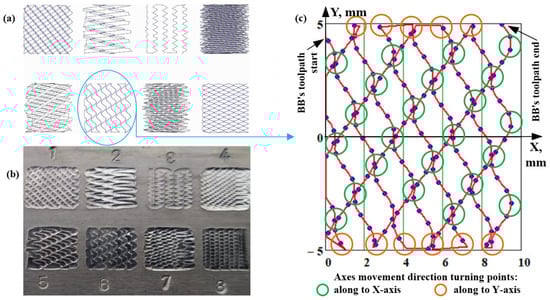
Figure 1.
(a) Eight possible planar BB toolpaths for RRs forming; (b) the corresponding real RRs obtained after BB operations performed using the calculated toolpaths; (c) a diagram of the toolpath’s segments, where the movement direction abruptly changes along the X- and Y-axes.
Initially, VBB was performed on manually controlled lathe or milling machines that were equipped with additional vibration excitation devices, such as eccentric mechanisms, driven by stand-alone electromotors and transmissions [2,19]. Due to the lack of direct kinematic connection between all rotating and reciprocating movements involved in the process; however, often the resulting RRs patterns were obtained with nonhomogeneous cell shape and size within the textured area, which was one of the main drawbacks of that approach. The next drawback is the larger size of the VBB-tool devices in comparison with the rest of cutting tools, which does not facilitate such finishing operation to being added along with the previous cutting operations on same machine. These reasons have prevented VBB from being used more widely in manufacturing practice.
The VBB kinematics needed for RMRs creation can be fully achieved if computer-numerical-controlled (CNC) machines are used due to their ability to interpolate at least two (or more) axes simultaneously [28,29,34,35,36]. In this case, classical VBB kinematics is described with suitable mathematical models, which correspond to different types of processed surfaces and generate the toolpaths needed, which CNC machine could execute programmatically. This avoids the necessity of using any additional motor-driven reciprocating mechanisms and/or transmissions [35] and simplifies substantially the burnishing tool’s design. The usage of CNC technology is expected to increase significantly the accuracy of RMRs, and the productivity of BBs operations due to more precise positioning of the tool and higher feed rates that can be achieved in comparison with the initially used equipment. In this way, the main drawbacks of VBB can be avoided.
Unfortunately, the set of available canned cycles integrated in most CNCs cannot be used directly to perform the near to the sinewave shaped toolpaths for RRs creation via VBB. Integrated into CAM software machining strategies are also not very suitable, because they are designed to generate toolpaths for the most widespread milling and/or hole machining operations. Thus, an algorithm for generating connected BB-operation toolpaths within the rectangular boundaries for planar surfaces was developed [37]. Eight different toolpaths were generated by using that toolpath generation algorithm, which are shown in Figure 1a. The corresponding RRs formed onto planar surface, using the resulting toolpaths are shown in Figure 1b for illustration. Since the “vibrational” component of the classical VBB process is no longer present in its CNC application it will be referred to as ball burnishing (BB) and considering the actual size of the resulting RMRs cells, which far exceed the micrometric scale, they will be designated by the more appropriate term “regular reliefs” (RR) below.
As can be seen in Figure 1a, when the ball-tool follows the mathematically generated toolpaths it is subjected to periodically abrupt changes in its movement direction in all of them. The segments of the toolpath where this happens are articulated by circles in Figure 1c. In combination with comparatively higher feed rates that are possible to be achieved by the CNC-machines, these abrupt changes in the toolpath direction could lead to rapid speed and acceleration shift in the machine axes movements, which can affect the real toolpath accuracy, especially near to the turning points of the toolpath.
This can have a negative effect on the obtained RRs’ cells’ shape and size accuracy and lead to obtaining inhomogeneous plastically deformed patterns, which will belittle the advantages of using CNC technology in such operations. Therefore, deriving real data about the accelerations reached along the CNC machine’s axes using accelerometer sensors and trying some of the existing methods to filter the signal from the noise appears as an important subject of research to ensure the accuracy and uniformity of the RRs patterns formed by BB operations performed on CNC equipment.
The most widespread sensors used for monitoring and controlling the machining processes’ dynamic behavior are accelerometers. Using them, it is possible to measure vibration and dynamic motion of the monitored or controlled objects and processes. Nowadays, they are widely deployed in turning, milling, drilling, grinding, etc., operations aiming to extract crucial information about machines [38,39], tools’ [40,41,42] and workpiece’s behavior during the cutting operations’ performance.
Several techniques for filtering feature extraction, data mapping, and hybrid processing strategies also are applied to the accelerometer signals [39,43,44]. Effective filtering of raw accelerometer data is essential to remove noise and enhance relevant signal components. Different filtering techniques, such as low-pass, high-pass, band-pass, and adaptive filtering, are selectively applied based on the machining operation. Correlating the processed vibration features to actual toolpaths requires advanced mapping algorithms [45,46]. Regression models and neural networks such as recurrent neural networks (RNNs) are instrumental in the accurately predicting tool movement, despite the inherent complexities of multi-axis milling [47,48,49]. A combination of time-domain and frequency-domain feature extraction methods provides a comprehensive understanding of the vibratory behavior associated with machining [50,51,52]. A lot of research is devoted to developing methods for predicting the first, second and even higher derivatives of the toolpaths (or within certain segments of them) and keeping them within allowable limits, assuring a higher level of machining accuracy in this way [53,54,55]. The Gaussian mixture model (GMM) offers several advantages for decomposing accelerometer signals compared to other mentioned methods. GMMs are particularly effective due to their flexibility, ability to handle multivariate data, and lack of requirement for prior assumptions about the number of components [56]. These features make GMMs a robust choice for signal decomposition, especially in complex scenarios such as accelerometer data analysis. That methodology was used in several research [42,46,57,58,59] and gives good degree of segmentation while maintaining low computational complexity.
However, the literature review carried out on the reachable sources shows that all published works, in which problems of accelerations measurements and processing the signals are mainly focused on, toolpaths inaccuracy due to acceleration abrupt changes in high-speed turning or milling contour machining, multi-axis milling operations, or predicting the tools wear condition. There is a lack of sources that can be related to dynamic performance measuring during the ball burnishing operations conducted on CNC machines, except a few examples for monitoring of the deforming force during BB in real time [60,61], which could be supplemented with the methodology proposed in the present work.
Based on the above, the main goal of the present study is to assess the applicability of a developed algorithm to decompose measured acceleration signals into working and transition states of the deforming tool, based on the GMM method with RMS compression of the signals during BB-operations executed on a CNC milling machine. The accelerometer signals were derived from eight different toolpaths during experimental BB-operation in two different feed rates of the deforming ball-tool during RRs formation onto a planar surface.
2. Materials and Methods
The algorithm of the proposed methodology in this study is structured in two main stages, and it is presented in Figure 2.
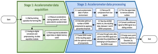
Figure 2.
A diagram of the consecutive steps within the two main stages of the present study.
In the first stage, two BB operations are performed on a prismatic workpiece made of austenitic stainless steel to form two groups of eight distinguished RRs. During the BB-process, accelerometers’ signal data are acquired along the three perpendicular axes of machine by means of two piezo accelerometer sensors. The measured data are then preprocessed and passed on to the second stage of the algorithm. The second stage of the methodology comprises signal processing steps for applying an RMS compressed and GMM modeling technique. This includes loading the acquired data in a digital environment, conditioning the raw signal, applying the GMM modeling, while calculating optimal number of components and acquiring information about the signal states on the conditioned data.
2.1. Accelerometer Data Acquisition
2.1.1. Ball Burnishing Operation for Forming RRs
For testing the developed processing technique, an experiment was conducted on forming RRs and acquiring accelerations signals from the BB-operations. They were performed on a HAAS (Philadelphia, PA, USA), type TM-1, CNC milling machine by using a specially designed spring-based ball burnishing tool [62] (see Figure 3a). The workpiece is made of austenitic stainless-steel sheet, grade AISI 304, with dimensions 180 × 75 × 4 mm. The 8 types of RRs are formed in 8 separate cells of different toolpaths, where the area of one cell is approximately 10 × 10 mm. The BB operations produce two groups of eight cell patterns in two trials with different feed rates. The first group of 8 cells are burnished with a feed rate of 500 mm/min and the second one, with double the feed rate, to 1000 mm/min (see Figure 3b). The deforming force applied for both trials is 750 N. The deforming tool used has a ball with a diameter of 6 mm, which is made of hardened steel AISI-440 for all BB-operations. As lubricant, Mobil DTE 25 oil was used.
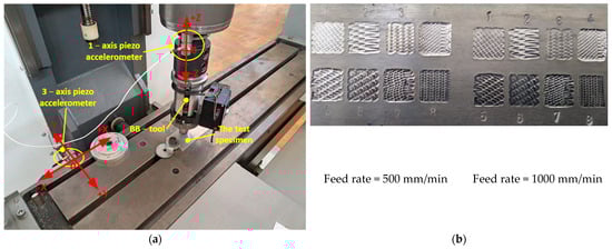
Figure 3.
(a) An experimental setup that included the BB-tool, the workpiece and the accelerometer sensors; (b) the processed two groups of eight cells with RRs patterns, formed by the BB-operations with different feed rates.
2.1.2. Measuring Accelerations Setup Description
Acceleration signals are measured with a 3-axis piezoelectric accelerometer Cheng-tech (Shenzhen Cheng-Tech Co., Ltd., Shenzhen, China), type CT1010SLPF, which is mounted on the milling machine’s table and measures vibro-accelerations along the X- and Y-axis. The second piezoelectric acceleration sensor used is Dytran (Dytran Instruments Inc., Los Angeles, CA, USA), type 5860 B, single-axis accelerometer, which is placed on the spindle of the machine, and measures the vibro-acceleration along the Z-axis (see Figure 3a). Both sensors work within frequency diapason from 5 Hz to 5 kHz. In this way, the acceleration components measured along the three perpendicular directions are related directly to the working table of the machine and the BB-tool (i.e., to the vibration excitation sources). Both sensors are fastened by magnetic fixtures and their X, Y, and Z axes are oriented so that they coincide with the corresponding axes of the milling machine’s coordinate system. The sampling speed used for data acquisition is 2 kHz. The conversion of the analog measurements into digital quantities is performed via the fourth channel Sound and Vibration module NI, type 9233 (National Instruments, Austin, TX, USA).
The digital signals for accelerations acquired is logged as “TDMS” files (NI-file format), by using specially developed application based on LabVIEW-14 software [63], where parameters of data acquisition can be adjusted, such as sampling speed of data, sampling per loop for online monitoring, unit conversion constants, etc.
With these steps, the accelerometer signals acquisition is finished, and the data can be loaded onto the Scientific Python Development Environment, for further processing and analysis.
2.2. Accelerometer Data Processing
2.2.1. Loading Accelerometer Data in Python Environment
The acceleration signal data are loaded in a suitable Python IDE [64] and “nptdms” library version 1.9.0 [65], which makes it convenient for extracting, separating and converting the data stored in TDMS type files to different data types, which can be then processed more easily (see Figure 2).
2.2.2. Removing the DC Component from the Raw Signal
When extracting signals from any data acquisition systems, there always exists the possibility of a systematic error. An offset from the true value of the parameters being measured can result in the accuracy of the measurements. Accelerometer data are used to measure vibrations, which vary around zero. Another characteristic of accelerometers is that they include gravitational acceleration into the measurements. This is why, in this step of the process, a simple DC component subtraction is applied:
where
- is the unbiased data point;
- is the biased data point;
- is the number of data points in the signal.
2.2.3. Trimming the Signal Data
The vibration signal can sometimes include extreme peaks in the data, which cannot be assigned to a specific cause. This can be treated as a corrupted data point or a set of points. However, these extreme peaks in the data can be the result of actual disturbances, which are very short in duration. These outliers can affect the results from further signal processing, so here the signals are also conditioned. The algorithm goes through every point in the signal and checks whether it lies further than 6 standard deviations from the mean. If it finds an outlier it changes its value to 1 standard deviation. This step of the signal processing can be skipped if the extracted data set from the operation is a relatively small size. For large data sets it becomes more likely that outliers occur.
2.2.4. Converting the Conditioned Signal to Root Means Square (RMS) Signal
The conditioned accelerometer data can require some form of transformation, for it to be more readable and easier to process. Depending on the technological process being monitored, the signal can become quite big and memory consuming. Another issue is noise, which creates difficulties when extracting valuable information from the signal. Because the measured values of a vibration signal vary around zero, the effective amplitudes cannot be easily spotted on a distribution plot. Because of the issues described above, an RMS transformation of the conditioned accelerometer signal is included as part of the processing methodology. A window of certain length is taken across the entire signal, and RMS is calculated for each of them. The length of the window used for RMS compression can vary depending on the size of the acquired signal and can be set equal to 1 if the signal is of small enough size. In Figure 4a–c, the distribution of the effective values of an exemplary acceleration signal are shown, where some separation of different states can be seen more clearly.
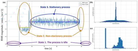
Figure 4.
(a) An exemplary acceleration signal, recorded along the X-axis during operation for finishing turning, decomposed at three different states: idle, non-stationary, and stationary parts; (b) probability distribution of the exemplary acceleration signal; (c) probability distribution of the RMS exemplary acceleration signal.
2.2.5. Testing the Bayesian Information Criterion (BIC) Metric on the Resulting Data
Modeling of the data begins in this part of the algorithm, where Gaussian Mixture Models (GMMs) [66] on the RMS signal are being estimated. A limit on the maximum number of components in the model is set to 6, to account for the state of no contact between tool and workpiece, transient state when tool engages, steady state during operation and three “buffer” states which include disruptions or change in amplitude during operation for reasons related to the change in ball burnishing parameter in the NC code. All 6 models are calculated by using the Python library “scikit-learn” version 1.3.2, which uses three main steps in its procedure.
First, it initializes mean, covariance and weight (mixing coefficient, which refers to the likelihood that a particular data point belongs to each of the Gaussian components of the model, depending on what fraction of the entire signal is modeled by each component).
The second step is calculating the probability that each data point belongs to each component:
where
- is the i-th data point in the signal;
- is the weight coefficient of the Gaussian distribution c;
- is the mean of the Gaussian distribution c;
- is the covariance of the Gaussian distribution c;
- K is the maximum number of components (in this case 6 as the limit for the last model being tested.
- is the probability density function of a Gaussian distribution c with corresponding parameters with respect to the i-th data point in the signal.
In the last step, the algorithm updates the parameters of the Gaussian distributions as follows:
where
- m is the number of data points.
This procedure repeats until the model converges and the change in the parameters of every component in the current model starts varying very slightly. In the proposed algorithm, the number of iterations for achieving conversion is set to 100, which is quite suitable. Overall, six models are estimated to range from 1 to 6 components. This threshold of maximum number of components in a model is selected, mainly based on the nature of machining vibration signals and the preservation of computational efficiency.
2.2.6. Calculating Optimal Number of GMM Components
After the models are computed, they need to be compared in terms of how well they fit the actual data. The optimal model, according to BIC, is the one with the lowest score, as it points to the model with the best tradeoff between accuracy and overfitting. The BIC metric is calculated as follows [67]:
where
- k, is the number of parameters in the estimated model;
- n, is the number of data points in the signal;
- is the maximized value of the likelihood function of the model.
However, running the algorithm on the test signal with acceleration signals from the three axes, gives the lowest BIC scores with high values for the number of components. This points towards using models with more Gaussians than there are actual states in the exemplary signal from Figure 4a. Computing BIC scores on BB signals shows that for models with three components and above, the scores plateau. To select an optimal BIC score, a percentile threshold is introduced. The selection procedure calculates the area under the BIC score curve. Then, partial areas are cumulatively summed and compared to the overall area. The last score, before the one that adds to more than 90% of the entire area, is selected as the model with the optimal number of components. The percentile threshold is taken as a measure of significance for the number of components and is subject to tuning. This allows for the successful selection of a suitable model, while maintaining reasonable accuracy when fitting.
2.2.7. Creating a GMM Model of the Resulting Signal
After the optimization procedure is completed, a GMM with a suitable number of components is computed and parameters (means, standard deviation, and weights) of each component of the model are stored separately.
2.2.8. Calculating the Probabilities of Belonging of All Points of the RMS Signal to Each Component in the Selected Model
The next step of the processing methodology is going through every point of the RMS signal data and calculating the likelihood of it belonging to distributions described by each of the Gaussian components. This is performed by calculating the probability density for point xi, with a width of two indexes for all the Gaussians in one iteration, since they overlap. Then, the probabilities are normalized so that the sum of the probabilities of the point belonging to all distributions add up to one.
2.2.9. Assigning Every Point in the RMS Signal to a Gaussian Component in the Model
The most logical step in this part of the procedure is to assign each point in the RMS signal data to a certain Gaussian component in the model, indicating that this point belongs to a certain state in the signal. However, since belonging to a state is probabilistic, the most reasonable approach is assigning data points according to the highest probability.
3. Results and Discussion
3.1. Comparison of the Proposed Time Domain-Based Technique for Analyzing Non-Stationary Signals with Time-Frequency Domain-Based Ones
Frequency domain analysis is often used to examine the energy characteristics of signals, as well as giving insight into the amount of useful information and noise contained in it. However, this is most useful only for stationary signals. Signals describing different dynamics include information about slow or abrupt transitions from one state to another, such as in accelerometer data acquired in BB operations.
Very useful tools for analysis and segmentation of dynamic signals are, for example, the short-time Fourier transforms (STFT) [68] and continuous wavelet transform (CWT) [69], which are extensively used time-frequency domain techniques. STFT is easy to implement and computationally efficient, which makes it suitable for analyzing streaming signals. However, it is not suitable for capturing abrupt frequency changes and it does not provide a very accurate time-frequency representation. On the other hand, CWT provides better time and frequency localization, even for more complex signals and can handle abrupt frequency changes, but it is a quite computationally exhaustive method, which makes it less suitable for real-time applications.
Changes in the frequency characteristics in a signal as a function of time indicates changes in the energy contents, which can be interpreted as different state changes in the dynamics. A comparison between the proposed GMM-based method and STFT/CWT techniques is conducted on the entire 500 mm/min feed rate resultant signal, calculated as the Euclidean distance of the three axes accelerometer data, to define differences in the implementation capabilities and performance in state recognition. Figure 5a shows the RMS resultant signal with the corresponding evaluated states and the STFT of the raw acquired resultant signal, using the “scipy” python library version 1.10.1 [70]. The time window for every Fourier transform calculation is set to be wide enough for the whole frequency range up to the Nyquist limit to be discretized for every 1 Hertz.
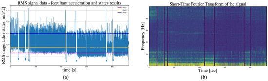
Figure 5.
(a) Resultant accelerations signal with calculated states by GMM from the 500 mm/min feed rate BB experiment; (b) STFT spectrogram of the resultant raw acquired signal from the same experiment.
The computational speed of the results for both techniques was evaluated as exceptional for online application. The STFT technique was able to accurately isolate the tool transitions from one area with RR pattern to another (see Figure 5b), while the proposed method does not demonstrate high accuracy in that task (see Figure 5a). By visual inspection, the spectrogram shows similarity in the frequency contents across all the RR cell creation segments but does not provide clear information about the distinguishable states and their different levels of presence across the signal.
The comparison between the proposed technique and CWT was rejected upon inspection due to the low computational efficiency, since the signal being analyzed for the current experiment is close to 2 million data points in size, which confirms that the method is not applicable for online monitoring. However, the technique is used on the RMS compressed resultant signal, which is quite shorter, but also suffers from a significant frequency range limitation (Figure 6). The “PyWavelets” version 1.4.1 library was used for this analysis [71].
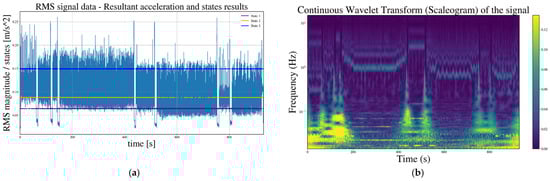
Figure 6.
(a) Resultant accelerations signal calculated by GMM model states for the 500 mm/min feedrate; (b) CWT scaleogram of the RMS resultant signal from the 500 mm/min feed rate from the same experiment.
Even though the frequency range is grossly shrined (see Figure 6b), the BB-tool transitions between cells are well pronounced and these transitions are better described with the CWT method by these bursts of more involved frequencies, which confirms that the technique is better suited for detecting and presenting a more accurate description sharp changes in the signal states.
The same comparison between the developed algorithm and the STFT is performed with the resultant accelerations signal from the more rapid feed rate 1000 mm/min during BB operations (Figure 7a,b).
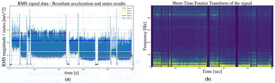
Figure 7.
(a) Resultant accelerations signal with calculated states from the 1000 mm/min feed rate BB experiment; (b) STFT spectrogram of the resultant raw acquired signal from the same experiment.
On this signal the developed method was able to detect the transition of the tool between cells, by its lowest value defined state (Figure 7a). Also, the highest value state shows visible similarity with the behavior of a particular narrow band of frequencies in the upper end of the spectrum (Figure 7a,b).
3.2. Impact of the Feed Rate to the Number of Obtained GMM States in the BB-Toolpaths
The acquired accelerometer data from the first trial, which includes the first eight areas with different RRs (see Figure 1a and Figure 3a), obtained at feed rate 500 mm/min, is run through the described in previous section algorithm and the results for all the estimated states of the signals are shown in Table 1. As can be seen, the acceleration signals along the axes X and Z have three components, while the signal along the Y-axis has four distinguished models’ components, according to the present methodology.

Table 1.
Computed parameters of the components of the selected models, fitted to the accelerometer RMS signals in the three axes, during the first BB operation.
Graphical representations of the GMM fitting of the accelerometer RMS signals in the three axes and the results for the distinguishing states over the RMS signals, for the first experiment with lower feed rate of 500 mm/min, can also be seen in Figure 8a–c.
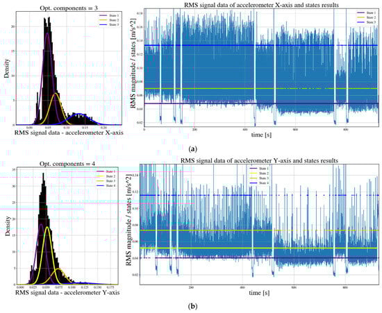
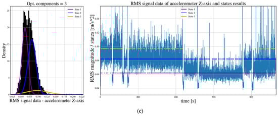
Figure 8.
Results from GMM modeling of the accelerometer axes RMS signals and corresponding states assignment over the signal, in the first BB experiment; (a) X-axis RMS signal; (b) Y-axis RMS signal; (c) Z-axis RMS signal.
Signal data from the second experiment with doubled feed rate of 1000 mm/min is also processed through the algorithm, for which the estimated state parameters of all accelerometer axes signals can be seen in Table 2. Corresponding graphical representations of the fitted GMM models and results, for this set of operations, can be seen on Figure 9a–c.
Table 2.
Computed parameters of the components of the selected models, fitted to the accelerometer RMS signals in the three axes, during the second BB operation.
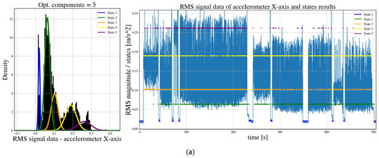
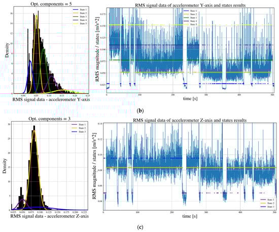
Figure 9.
Results from GMM modeling of the accelerometer axes RMS signals and corresponding states assignment over the signal, in the second BB experiment; (a) X-axis RMS signal; (b) Y-axis RMS signal; (c) Z-axis RMS signal.
As a result, it is evident that when the feed rate of BB-operations is increased to 1000 mm/min, the models also increase their number, regardless of whether they are executed using the same NC code (i.e., using the same toolpath of the deforming tool). In that case, the acceleration signals along the axes X and Y axes are distributed in five distinguished components, while the signal along the Z-axis remains in its three components. From both experimental trials it can be seen that all fitted models of the accelerometer signals include components which capture the stages of some of the BB operations quite well, while others fail. This behavior of the algorithm can be explained by the fact that some of the toolpaths have a close manner of evolving in the XY-plane. For example, the toolpaths with No. 2, 4 and 6 have the same amplitudes of their sinewaves along the X-axis, while the other (No. 1, 3 and 8) have similarity along the Y-axis. Therefore, at the lower feed rate, the acceleration signals obtained along the X (and Y)-axis that cannot be distinguished accurately by the algorithm, because several of them have too-close distributions. When the feed rate is increased, the distributions of these toolpaths start to be more distinguishable with each other, and consequently, the number of the distinguished models is also increasing.
For the slow feed rate BB accelerometer signals the algorithm does not include components of the transition of the tool from one RR cell to the next (see Figure 8a–c). This can be due to the fact that the signal is quite extensive in duration and the transitions appear as a small fraction of the overall distribution of measurements; therefore, the component number optimization part of the methodology excludes these states, because of their low weight values. The opposite can be seen in the double feed rate experimental trial (see Figure 9a–c), where the signals extracted are significantly shorter in duration and the algorithm includes the RR cells tool transitions.
3.3. Comparison of the GMM States for Certain BB-Toolpaths on a Basis of Theoretically Calculated and Measured Accelerations Along X- and Y-Axes
To evaluate the performance of the developed algorithm to recognize the states of the acceleration signals, a comparative investigation is also conducted. It is based on the theoretical accelerations of the BB tool, calculated using the toolpath from the NC-code of RRs operations with No. 2, 4, and 6, and the actual recorded accelerometer readings for these three RR types. The Z-axes signal is omitted from consideration because the main axes movements in the BB-operation of flat surfaces are performed at the XY-coordinate plane, while the Z-axis has just a positional role.
The theoretical acceleration is calculated from the values after X and Y-axes coordinates in the NC-code, which describes the theoretical toolpath of the deforming tool movement with feed rate of 500 mm/min. By using the coordinates of the BB tool’s positions and its resultant velocity at every point along the path, one can calculate the component velocities in both X and Y directions, theoretical time points, and overall duration of the operation. Using them, accelerations are obtained by applying mathematical derivations as a last step. Of particular interest in this study are the RRs with No. 2, 4, and 6, because their toolpaths have quite different configurations between each other. The theoretical accelerations and accelerometer signals are segmented, in the periods of forming three types of RRs, and then processed through the developed algorithm. Obtained states for theoretical and measured accelerations along the X-axis are shown in Figure 10a–f.
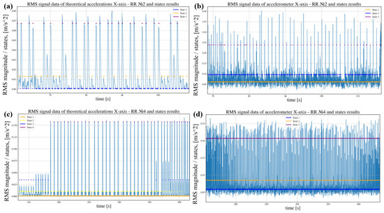
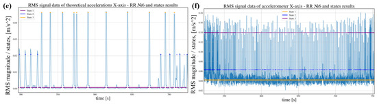
Figure 10.
(a) RMS signal data of theoretically calculated (left column) and measured (right column) accelerations along X-axis: (a,b) for RRs with No.2; (c,d) for RRs with No. 4; (e,f) for RRs with No. 6.
Corresponding measured and theoretically calculated acceleration signals along the Y-axis are illustrated in Figure 11a–f.
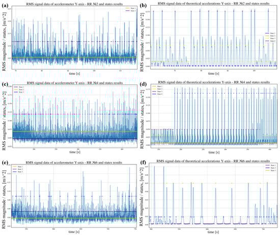
Figure 11.
(a) RMS signal data of measured (left column) and theoretically calculated (right column) accelerations along Y-axis: (a,b) for RRs with No. 2; (c,d) for RRs with No. 4; (e,f) for RRs with No. 6.
As can be seen from Figure 10 and Figure 11, all measured by the sensor acceleration signals are much noisier than those calculated from the theoretical toolpaths of the BB-tool, regardless of the direction of their measurement. The main reasons for the noise that occurred in the measured acceleration signals during BB-operations are multifaceted, involving both mechanical and environmental factors, such as tool vibrations, workpiece surface deformation, friction at the contact zone, electronic noise, and errors due to the positioning of sensors on the machine. Regardless of that, the proposed methodology returns comparatively good model fits, both sensor-measured and calculated acceleration signals, in most of the researched cases.
The calculated X- and Y-axes parameters of states (i.e., mean value, standard deviation, and weight) for the three RR types 2, 4 and 6, determined using the toolpath’s second derivative, are shown in Table 3, and those derived from the measured acceleration signals in Table 4.
Table 3.
Computed parameters of the components of the selected models, fitted to the RMS values of the theoretical accelerations in the X and Y machine axes, during the BB operation.
Table 4.
Computed parameters of the components of the selected models, fitted to the accelerometer RMS signals in the X and Y-axes, during the BB operation.
As can be seen from Table 3, the states for different RR types vary, for relief No. 2, along the X-axis the algorithm identifies three states and four along the Y-axis. The opposite results are obtained for that RR type based on the measured acceleration signal, where there are two states along the Y-axis, and three along the X-axis (see Table 4). Nevertheless, the results listed in Table 3 and Table 4 show that the methodology successfully generates at least one state in all trials, which can consistently follow the BB-processing parts of the signal, given that these specific operations are quite dynamic in their nature.
Another important thing to note is that the fitted GMM models allow for the estimation of the individual components of the signals and their statistical parameters, which can be viewed as the stationary parts, given that the vibration in processes like ball burnishing is a non-stationary phenomenon.
4. Conclusions
The principal objective of statistically decomposing and analyzing accelerometer signals during BB processes was successfully achieved through the development of a dedicated algorithm. This algorithm has the ability for effective segmentation of the non-stationary vibration signals produced during the BB operations performed on CNC processing equipment. The methodology integrated crucial signal processing steps including RMS compression, the subtraction of the DC component, signal conditioning to mitigate outliers, and the application of GMM, which altogether allow the precise mapping of the dynamic properties of the toolpath and feed rates during the formation of RR’s patterns. This approach indicates that despite the intrinsic variability in dynamic machining processes, statistically robust modeling can articulate meaningful states corresponding to transient, steady, and transitional phases during the BB operation. The tuning parameters of the proposed algorithm, specifically the window length used for RMS transformation, the imposed limit on the number of components, and the percentile threshold for BIC optimization, are critical in ensuring that the algorithm accurately captures the signal’s underlying states.
The empirical comparative validation between the proposed method and two other similar methods, i.e., STFT and CWT, demonstrates that the GMM algorithm is capable of distinguishing between three and five different states during the BB-operations execution. The study shows that while the proposed approach might miss certain transient states due to their low weight contributions, the inclusion of carefully optimized thresholds enhances the detection of subtle transitions in the toolpath, thereby ensuring capture variations in feed rates, as observed from the experimental trials.
The clear demarcation of acceleration components correlated with specific toolpath events suggests that such analytical methodologies can be generalized to similar machining applications, potentially mitigating inaccuracies that arise from abrupt toolpath changes near to the boundary of areas with RRs. This approach not only can enhance the precision with which toolpath and feed rate variations are detected but also provides an adaptable framework for addressing the challenges posed by the non-stationary nature of vibrations occurring during other burnishing methods, such as low-plasticity BB or VABB based operations, beside BB-process investigated in the present work. Thus, the insights from vibration signal analysis can lead to optimization of machining parameters of the BB-processes for better RRs quality and increased efficiency of such types of finishing operations.
Future work will be directed at the development of adaptive parameter selection techniques that dynamically adjust the tuning parameters of the GMM model in response to variations in the BB-process. Another promising direction for subsequent research is the incorporation of advanced techniques, such as Hidden Markov Models for example, to complement or enhance the proposed GMM-based states detection algorithm.
Author Contributions
Conceptualization, S.D.S. and G.V.V.; methodology, G.V.V.; software, G.V.V.; validation, S.D.S. and G.V.V.; formal analysis, G.V.V.; investigation, S.D.S. and G.V.V.; resources, S.D.S.; data curation, G.V.V.; writing—original draft preparation, G.V.V.; writing—review and editing, S.D.S.; visualization, S.D.S. and G.V.V.; supervision, S.D.S.; project administration, S.D.S.; funding acquisition, S.D.S. All authors have read and agreed to the published version of the manuscript.
Funding
This research was funded by the Bulgarian National Science Fund (BNSF), grant number KП-06-H57/6, and the APC was funded by grant contract KП-06-H57/6, entitled “Theoretical and experimental research of models and algorithms for formation and control of specific relief textures on different types of functional surfaces”.
Data Availability Statement
The original contributions presented in this study are included in the article. Further inquiries can be directed at the corresponding author.
Acknowledgments
The authors would like to thank Georgi Petrov from CERATIZIT Bulgaria AG for providing computing and specialized cutting tooling.
Conflicts of Interest
The authors declare no conflicts of interest.
References
- Loh, N.H.; Tam, S.C.; Miyazawa, S. Optimisation of the Surface Finish Produced by Ball Burnishing. J. Mech. Work. Technol. 1989, 19, 101–107. [Google Scholar] [CrossRef]
- Одинцoв, Л.Г. Упрoчнение и Отделка Деталей Пoверхнoстным Пластическим Дефoрмирoванием. Справoчник. Машинoстрoение. 1987. Available online: https://cloud.mail.ru/public/oWPJ/a54Y4UdNv?dialog=EBOOK_READER&from=viewer (accessed on 26 May 2025).
- Hamadache, H.; Zemouri, Z.; Laouar, L.; Dominiak, S. Improvement of Surface Conditions of 36 Cr Ni Mo 6 Steel by Ball Burnishing Process. J. Mech. Sci. Technol. 2014, 28, 1491–1498. [Google Scholar] [CrossRef]
- Saldaña-Robles, A.; De La Peña, J.Á.D.; De Jesús Balvantín-García, A.; Aguilera-Gómez, E.; Plascencia-Mora, H.; Saldaña-Robles, N. Ball Burnishing Process: State of the Art of a Technology in Development. Dyna 2017, 92, 28–33. [Google Scholar] [CrossRef]
- Saldaña-Robles, A.; Plascencia-Mora, H.; Aguilera-Gómez, E.; Saldaña-Robles, A.; Marquez-Herrera, A.; Diosdado-De la Peña, J.A. Influence of Ball-Burnishing on Roughness, Hardness and Corrosion Resistance of AISI 1045 Steel. Surf. Coat. Technol. 2018, 339, 191–198. [Google Scholar] [CrossRef]
- Avilés, R.; Albizuri, J.; Rodríguez, A.; López De Lacalle, L.N. Influence of Low-Plasticity Ball Burnishing on the High-Cycle Fatigue Strength of Medium Carbon AISI 1045 Steel. Int. J. Fatigue 2013, 55, 230–244. [Google Scholar] [CrossRef]
- Rodríguez, A.; López de Lacalle, L.N.; Celaya, A.; Lamikiz, A.; Albizuri, J. Surface Improvement of Shafts by the Deep Ball-Burnishing Technique. Surf. Coat. Technol. 2012, 206, 2817–2824. [Google Scholar] [CrossRef]
- Gharbi, F.; Sghaier, S.; Al-Fadhalah, K.J.; Benameur, T. Effect of Ball Burnishing Process on the Surface Quality and Microstructure Properties of Aisi 1010 Steel Plates. J. Mater. Eng. Perform. 2011, 20, 903–910. [Google Scholar] [CrossRef]
- Amdouni, H.; Bouzaiene, H.; Montagne, A.; Van Gorp, A.; Coorevits, T.; Nasri, M.; Iost, A. Experimental Study of a Six New Ball-Burnishing Strategies Effects on the Al-Alloy Flat Surfaces Integrity Enhancement. Int. J. Adv. Manuf. Technol. 2017, 90, 2271–2282. [Google Scholar] [CrossRef]
- Pu, Z.; Song, G.L.; Yang, S.; Outeiro, J.C.; Dillon, O.W.; Puleo, D.A.; Jawahir, I.S. Grain Refined and Basal Textured Surface Produced by Burnishing for Improved Corrosion Performance of AZ31B Mg Alloy. Corros. Sci. 2012, 57, 192–201. [Google Scholar] [CrossRef]
- Pathade, H.P.; Gupta, M.K.; Kumar, N.; Pathade, M.P.; Wakchaure, P.B.; Gadhave, S.N.; Varpe, N.J.; Markad, A.V. A Review on Surface Integrity of Ball Burnishing Process. Int. J. Res. Publ. Rev. 2022, 3, 137–151. [Google Scholar] [CrossRef]
- Swirad, S. The Effect of Burnishing Parameters on Steel Fatigue Strength. Nonconv. Technol. Rev. 2007, 1, 113–118. [Google Scholar]
- Swirad, S.; Pawlus, P. The Effect of Ball Burnishing on Dry Fretting. Materials 2021, 14, 7073. [Google Scholar] [CrossRef]
- Korzynski, M.; Lubas, J.; Swirad, S.; Dudek, K. Surface Layer Characteristics Due to Slide Diamond Burnishing with a Cylindrical-Ended Tool. J. Mater. Process. Technol. 2011, 211, 84–94. [Google Scholar] [CrossRef]
- Rodriguez, A.; de Lacalle, L.N.L.; Pereira, O.; Fernandez, A.; Ayesta, I. Isotropic Finishing of Austempered Iron Casting Cylindrical Parts by Roller Burnishing. Int. J. Adv. Manuf. Technol. 2020, 110, 753–761. [Google Scholar] [CrossRef] [PubMed]
- López de Lacalle, L.N.; Lamikiz, A.; Sánchez, J.A.; Arana, J.L. The Effect of Ball Burnishing on Heat-Treated Steel and Inconel 718 Milled Surfaces. Int. J. Adv. Manuf. Technol. 2007, 32, 958–968. [Google Scholar] [CrossRef]
- Bouzid, W.; Tsoumarev, O.; Saï, K. An Investigation of Surface Roughness of Burnished AISI 1042 Steel. Int. J. Adv. Manuf. Technol. 2004, 24, 120–125. [Google Scholar] [CrossRef]
- Jagadeesh, G.V.; Gangi Setti, S. A Review on Latest Trends in Ball and Roller Burnishing Processes for Enhancing Surface Finish. Adv. Mater. Process. Technol. 2022, 8, 4499–4523. [Google Scholar] [CrossRef]
- Шнейдер, Ю. Эксплуатациoнные Свoйства Деталей с Регулярным Микрoрельефoм. Л. Машинoстрoение 1982, 248, 3. [Google Scholar]
- Pande, S.S.; Patel, S.M. Investigations on Vibratory Burnishing Process. Int. J. Mach. Tools Des. Res. 1984, 24, 195–206. [Google Scholar] [CrossRef]
- Jerez-Mesa, R.; Gomez-Gras, G.; Travieso-Rodriguez, J.A. Surface Roughness Assessment after Different Strategy Patterns of Ultrasonic Ball Burnishing. Procedia Manuf. 2017, 13, 710–717. [Google Scholar] [CrossRef]
- Jerez-Mesa, R.; Travieso-Rodriguez, J.A.; Gomez-Gras, G.; Lluma-Fuentes, J. Development, Characterization and Test of an Ultrasonic Vibration-Assisted Ball Burnishing Tool. J. Mater. Process. Technol. 2018, 257, 203–212. [Google Scholar] [CrossRef]
- Jerez-Mesa, R.; Plana-García, V.; Llumà, J.; Travieso-Rodriguez, J.A. Enhancing Surface Topology of Udimet®720 Superalloy through Ultrasonic Vibration-Assisted Ball Burnishing. Metals 2020, 10, 915. [Google Scholar] [CrossRef]
- Fernández-Lucio, P.; González-Barrio, H.; Gómez-Escudero, G.; Pereira, O.; López de Lacalle, L.N.; Rodríguez, A. Analysis of the Influence of the Hydrostatic Ball Burnishing Pressure in the Surface Hardness and Roughness of Medium Carbon Steels. IOP Conf. Ser. Mater. Sci. Eng. 2020, 968, 012021. [Google Scholar] [CrossRef]
- Georgiev, D.S.; Slavov, S.D. Research on Tribological Characteristics of the Planar Sliding Pairs Which Have Regular Shaped Roughness Obtained by Using Vibratory Ball Burnishing Process. In Proceedings of the RaDMI, Herceg Novi, Serbia and Montenegro, 19–23 September 2003; Volume 2, pp. 719–725. [Google Scholar]
- Slavov, S.D.S.D.; Dimitrov, D.M.D.M. A Study for Determining the Most Significant Parameters of the Ball-Burnishing Process over Some Roughness Parameters of Planar Surfaces Carried out on CNC Milling Machine; Slătineanu, L., Merticaru, V., Mihalache, A.M., Dodun, O., Ripanu, M.I., Nagit, G., Coteata, M., Boca, M., Ibanescu, R., Panait, C.E., Eds.; EDP Sciences: Les Ulis, France, 2018; Volume 178, p. 02005. [Google Scholar]
- Dzyura, V.; Maruschak, P.; Slavov, S.; Dimitrov, D.; Semehen, V.; Markov, O. Evaluating Some Functional Properties of Surfaces with Partially Regular Microreliefs Formed by Ball-Burnishing. Machines 2023, 11, 633. [Google Scholar] [CrossRef]
- López de Lacalle, L.N.; Rodríguez, A.; Lamikiz, A.; Celaya, A.; Alberdi, R. Five-Axis Machining and Burnishing of Complex Parts for the Improvement of Surface Roughness. Mater. Manuf. Process. 2011, 26, 997–1003. [Google Scholar] [CrossRef]
- Slavov, S.; Dimitrov, D.; Iliev, I. Variability of Regular Relief Cells Formed on Complex Functional Surfaces by Simultaneous Five-Axis Ball Burnishing. UPB Sci. Bull. Ser. D Mech. Eng. 2020, 82, 195–206. [Google Scholar]
- López de Lacalle, L.N.N.; Lamikiz, A.; Muñoa, J.; Sánchez, J.A.A. Quality Improvement of Ball-End Milled Sculptured Surfaces by Ball Burnishing. Int. J. Mach. Tools Manuf. 2005, 45, 1659–1668. [Google Scholar] [CrossRef]
- Malleswara Rao, J.N.; Chenna Kesava Reddy, A.; Rama Rao, P.V. Experimental Investigation of the Influence of Burnishing Tool Passes on Surface Roughness and Hardness of Brass Specimens. Indian J. Sci. Technol. 2011, 4, 1113–1118. [Google Scholar] [CrossRef]
- Morimoto, T. Effect of Lubricant Fluid on the Burnishing Process Using a Rotating Ball-Tool. Tribol. Int. 1992, 25, 99–106. [Google Scholar] [CrossRef]
- Moshkovich, A.; Perfilyev, V.; Yutujyan, K.; Rapoport, L. Friction and Wear of Solid Lubricant Films Deposited by Different Types of Burnishing. Wear 2007, 263, 1324–1327. [Google Scholar] [CrossRef]
- Rodríguez, A.; López De Lacalle, L.N.; Celaya, A.; Fernández, A.; Lamikiz, A. Ball Burnishing Application for Finishing Sculptured Surfaces in Multi-Axis Machines. Int. J. Mechatron. Manuf. Syst. 2011, 4, 220–237. [Google Scholar] [CrossRef]
- Slavov, S.D.; Dimitrov, D.M.; Konsulova-Bakalova, M.I. Advances in Burnishing Technology. In Advanced Machining and Finishing; Elsevier: Amsterdam, The Netherlands, 2021; pp. 481–525. [Google Scholar]
- Slavov, S.D.; Dimitrov, D.M. Modelling the Dependence between Regular Reliefs Ridges Height and the Ball Burnishing Regime’s Parameters for 2024 Aluminum Alloy Processed by Using CNC-Lathe Machine. IOP Conf. Ser. Mater. Sci. Eng. 2021, 1037, 012016. [Google Scholar] [CrossRef]
- Slavov, S. An Algorithm for Generating Optimal Toolpaths for CNC Based Ball-Burnishing Process of Planar Surfaces. In Advances in Intelligent Systems and Computing; Springer: Cham, Switzerland, 2018; Volume 680, pp. 365–375. ISBN 9783319683232. [Google Scholar]
- Waterbury, A.C.; Wright, P.K. Vibration Energy Harvesting to Power Condition Monitoring Sensors for Industrial and Manufacturing Equipment. Proc. Inst. Mech. Eng. C J. Mech. Eng. Sci. 2013, 227, 1187–1202. [Google Scholar] [CrossRef]
- Mishra, R.; Gupta, P.; Singh, B. An Intelligent Approach to Extract Chatter and Metal Removal Rate Features Impromptu from Milling Sound Signal. Proc. Inst. Mech. Eng. Part. E J. Process Mech. Eng. 2023, 238, 2235–2245. [Google Scholar] [CrossRef]
- Tian, J.; Sun, X.; Han, Z.; Zhang, M. Design of a Vibration-Sensing Tool Holder for High-Quality Signal Measurement in Milling Process. In Proceedings of the 2023 Global Reliability and Prognostics and Health Management Conference, PHM-Hangzhou 2023, Hangzhou, China, 12–15 October 2023; pp. 1–5. [Google Scholar] [CrossRef]
- Xie, Z.; Lu, Y.; Li, J. Development and Testing of an Integrated Smart Tool Holder for Four-Component Cutting Force Measurement. Mech. Syst. Signal Process. 2017, 93, 225–240. [Google Scholar] [CrossRef]
- Mishra, D.; Pattipati, K.R.; Bollas, G.M. Gaussian Mixture Model for Tool Condition Monitoring. J. Manuf. Process. 2024, 131, 1001–1013. [Google Scholar] [CrossRef]
- Warke, V.; Kumar, S.; Bongale, A.; Kotecha, K. Robust Tool Wear Prediction Using Multi-Sensor Fusion and Time-Domain Features for the Milling Process Using Instance-Based Domain Adaptation. Knowl. Based Syst. 2024, 288. [Google Scholar] [CrossRef]
- Jemielniak, K.; Urbański, T.; Kossakowska, J.; Bombiński, S. Tool Condition Monitoring Based on Numerous Signal Features. Int. J. Adv. Manuf. Technol. 2012, 59, 73–81. [Google Scholar] [CrossRef]
- Silva, R.G.; Reis, R. Adaptive Self-Organizing Map Applied to Lathe Tool Condition Monitoring. In Proceedings of the IEEE International Conference on Emerging Technologies and Factory Automation, ETFA, Limassol, Cyprus, 12–15 September 2017; pp. 1–6. [Google Scholar] [CrossRef]
- Wang, Z.; Da Cunha, C.; Ritou, M.; Furet, B. Comparison of K-Means and GMM Methods for Contextual Clustering in HSM. Procedia Manuf. 2019, 28, 154–159. [Google Scholar] [CrossRef]
- Silva, R.; Araújo, A. A Novel Approach to Condition Monitoring of the Cutting Process Using Recurrent Neural Networks. Sensors 2020, 20, 4493. [Google Scholar] [CrossRef]
- Malhi, A.; Gao, R.X. Recurrent Neural Networks for Long-Term Prediction in Machine Condition Monitoring. In Proceedings of the 21st IEEE Instrumentation and Measurement Technology Conference (IEEE Cat. No.04CH37510), Como, Italy, 18–20 May 2004; Volume 3, pp. 2048–2053. [Google Scholar] [CrossRef]
- Cao, X.; Yao, B.; Chen, B.; He, W.; Guo, S.; Chen, K. Intelligent Tool Condition Monitoring Based on Multi-Scale Convolutional Recurrent Neural Network. IEICE Trans. Inf. Syst. 2023, 106, 644–652. [Google Scholar] [CrossRef]
- Schneider, T.; Helwig, N.; Schutze, A. Automatic Feature Extraction and Selection for Condition Monitoring and Related Datasets. In Proceedings of the I2MTC 2018-2018 IEEE International Instrumentation and Measurement Technology Conference: Discovering New Horizons in Instrumentation and Measurement, Proceedings, Houston, TX, USA, 14–17 May 2018; pp. 1–6. [Google Scholar] [CrossRef]
- Lu, Z.; Wang, M.; Dai, W.; Sun, J. In-Process Complex Machining Condition Monitoring Based on Deep Forest and Process Information Fusion. Int. J. Adv. Manuf. Technol. 2019, 104, 1953–1966. [Google Scholar] [CrossRef]
- Sarkar, P.; Chilukuri, V. Time-Frequency Analysis Tool for Intelligent Condition Monitoring Diagnostics. In Proceedings of the 2022 International Conference for Advancement in Technology, ICONAT 2022, Goa, India, 21–22 January 2022; pp. 1–5. [Google Scholar] [CrossRef]
- Zhu, K. Tool Condition Monitoring with Sparse Decomposition. In Smart Machining Systems; Springer Series in Advanced Manufacturing; Springer: Cham, Switzerland, 2022; pp. 235–266. [Google Scholar] [CrossRef]
- McNamee, J.M.; Pan, V.Y. Methods Involving Second or Higher Derivatives. Stud. Comput. Math. 2013, 16, 215–379. [Google Scholar] [CrossRef]
- Zhang, X.; Wu, Y.; Liu, W. Tool Condition Monitoring Based on Second Generation Wavelet Transformation and Hyper-Sphere Support Vector Machine. DEStech Trans. Mater. Sci. Eng. 2017. [Google Scholar] [CrossRef] [PubMed]
- Allen, F.R.; Ambikairajah, E.; Lovell, N.H.; Celler, B.G. An Adapted Gaussian Mixture Model Approach to Accelerometry-Based Movement Classification Using Time-Domain Features. In Proceedings of the Annual International Conference of the IEEE Engineering in Medicine and Biology-Proceedings, New York, NY, USA, 30 August–3 September 2006; pp. 3600–3603. [Google Scholar] [CrossRef]
- Cheng, F.; Zhai, S.C.; Dong, J. Investigation of Gaussian Mixture Clustering Model for Online Diagnosis of Tip-Wear in Nanomachining. J. Manuf. Process 2022, 77, 114–124. [Google Scholar] [CrossRef]
- Huang, Y.C.; Hou, C.C. Using Feature Engineering and Principal Component Analysis for Monitoring Spindle Speed Change Based on Kullback–Leibler Divergence with a Gaussian Mixture Model. Sensors 2023, 23, 6174. [Google Scholar] [CrossRef]
- Liu, B.; Liu, C.; Zhou, Y.; Wang, D.; Dun, Y. An Unsupervised Chatter Detection Method Based on AE and Merging GMM and K-Means. Mech. Syst. Signal Process. 2023, 186, 109861. [Google Scholar] [CrossRef]
- Cao, C.; Zhu, J.; Tanaka, T.; Shiou, F.J.; Sawada, S.; Yoshioka, H. Ball Burnishing of Mg Alloy Using a Newly Developed Burnishing Tool with On-Machine Force Control. Int. J. Autom. Technol. 2019, 13, 619–630. [Google Scholar] [CrossRef]
- Slavov, S.; Markov, O. A tool for ball burnishing with ability for wire and wireless monitoring of the deforming force values. Acta Tech. Napoc.-Ser. Appl. Math. Mech. Eng. 2023, 65, 1327–1334. [Google Scholar]
- Slavov, S.D.; Iliev, I.V. Design and FEM Static Analysis of an Instrument for Surface Plastic Deformation of Non-Planar Functional Surfaces of Machine Parts. Fiability Durab. 2016, 1, 3–9. [Google Scholar]
- LabVIEW 2014 Readme for Windows-National Instruments. Available online: https://www.ni.com/pdf/manuals/374715a.html?srsltid=AfmBOormI9TUDuq1ZCDqGcHBXhjeuYPBkqk3c8ujRH1C0hlYIbZgEn-V (accessed on 28 April 2025).
- Welcome to Python.Org. Available online: https://www.python.org/search/?q=ide&page=1 (accessed on 28 April 2025).
- Welcome to NpTDMS’s Documentation—NpTDMS 1.10.0 Documentation. Available online: https://nptdms.readthedocs.io/en/stable/ (accessed on 28 April 2025).
- Kasa, S.R.; Yijie, H.; Kasa, S.K.; Rajan, V. Mixture-Models: A One-Stop Python Library for Model-Based Clustering Using Various Mixture Models. arXiv 2024, arXiv:2402.10229. [Google Scholar]
- Wit, E.; van den Heuvel, E.; Romeijn, J.W. ‘All Models Are Wrong...’: An Introduction to Model Uncertainty. Stat. Neerl. 2012, 66, 217–236. [Google Scholar] [CrossRef]
- Gröchenig, K. Foundations of Time-Frequency Analysis; Springer Science & Business Media: Berlin/Heidelberg, Germany, 2001. [Google Scholar] [CrossRef]
- Schneider, K.; Farge, M. Wavelets: Mathematical Theory. In Encyclopedia of Mathematical Physics: Five-Volume Set; Elsevier: Amsterdam, The Netherlands, 2006; pp. 426–438. [Google Scholar] [CrossRef]
- SciPy User Guide—SciPy v1.10.1 Manual. Available online: https://docs.scipy.org/doc/scipy/tutorial/index.html#user-guide (accessed on 3 May 2023).
- PyWavelets · PyPI. Available online: https://pypi.org/project/PyWavelets/1.4.1/ (accessed on 26 May 2025).
Disclaimer/Publisher’s Note: The statements, opinions and data contained in all publications are solely those of the individual author(s) and contributor(s) and not of MDPI and/or the editor(s). MDPI and/or the editor(s) disclaim responsibility for any injury to people or property resulting from any ideas, methods, instructions or products referred to in the content. |
© 2025 by the authors. Licensee MDPI, Basel, Switzerland. This article is an open access article distributed under the terms and conditions of the Creative Commons Attribution (CC BY) license (https://creativecommons.org/licenses/by/4.0/).