
Computed Tomography-Based Volumetric Additive Manufacturing: Development of a Model Based on Resin Properties and Part Size Interrelationship—Part I


Abstract
1. Introduction
2. Analytical Approach
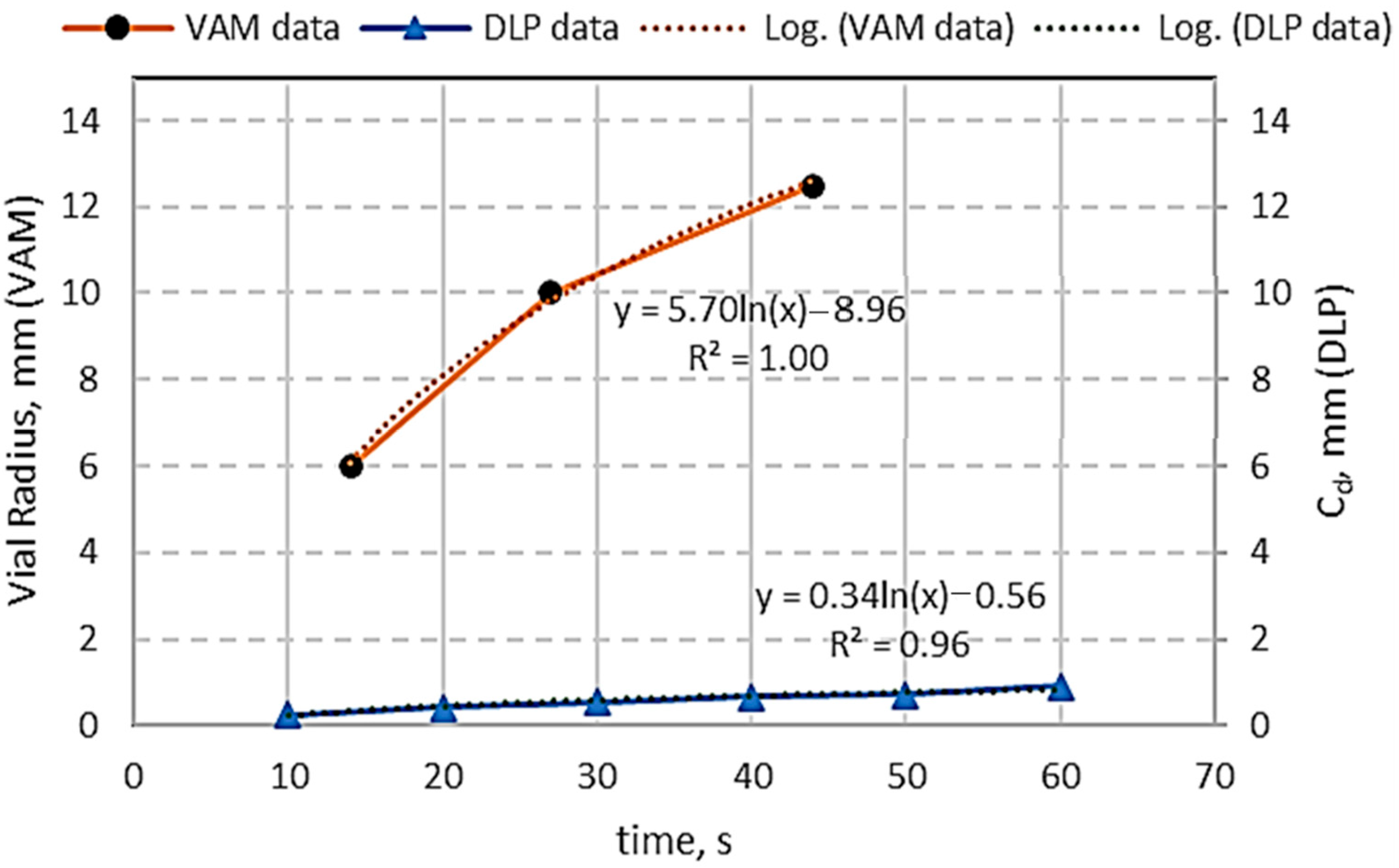
2.1. Obtaining Dp for the VAM Process
2.2. VAM Analysis—Uniform Light Intensity
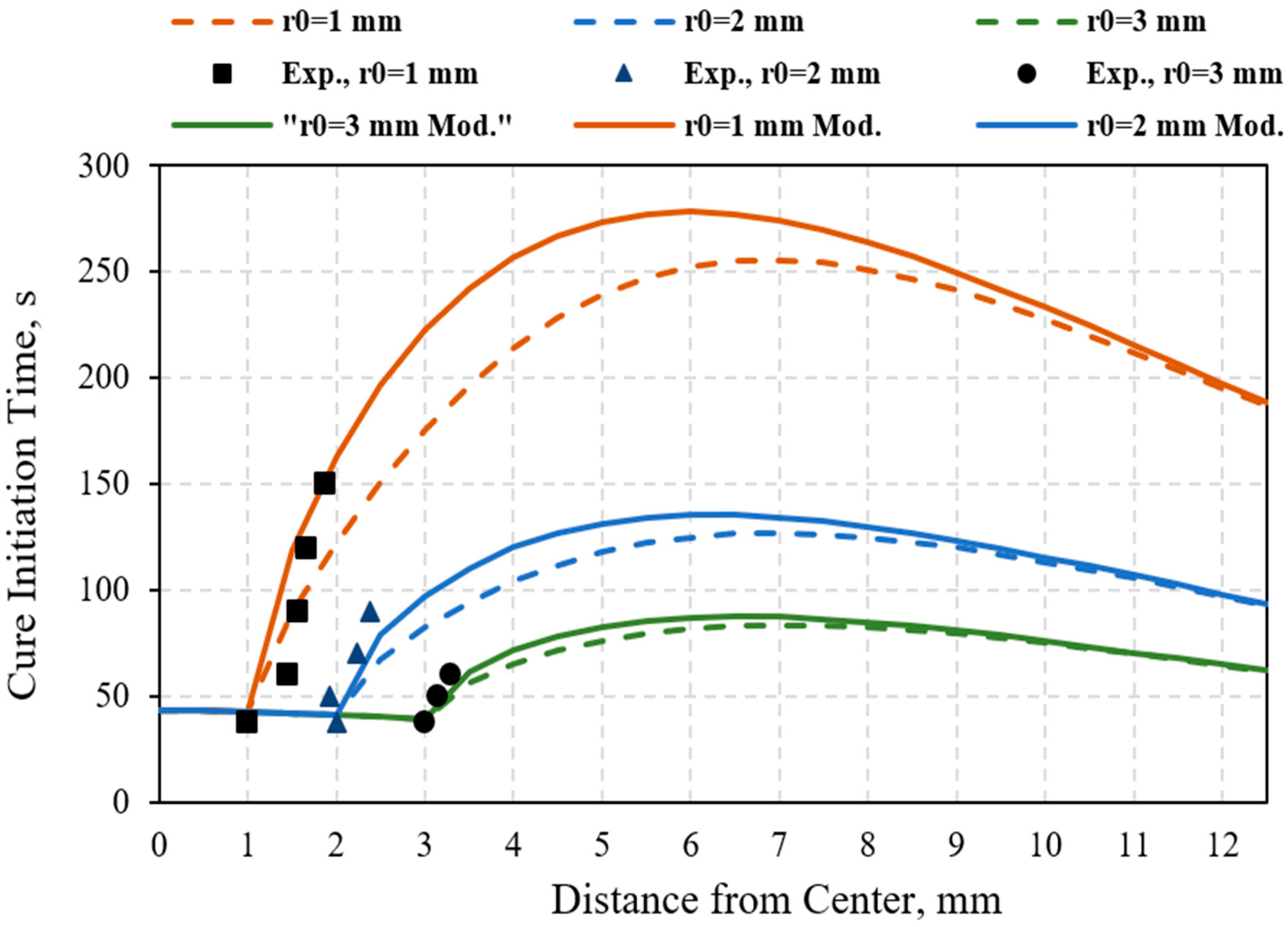
2.3. Numerical Analysis—Object Growth
2.4. A Consideration on Rotational Speed
3. Experimental Materials and Preparation
3.1. Experimental Setup
3.2. Experimental Design
4. Results and Discussion
4.1. Depth of Penetration, Dp
4.2. Experimental Verification
- Object Growth:
5. Conclusions
- The Dp, is a crucial factor in the analysis and experimentation in the VAM process. Its action and value are fundamentally different from the one obtained by the conventional AM polymerization methods, such as SLA and DLP. Thus, a method for its measurement and analysis is introduced for the VAM process. The value was found to be about one order of magnitude larger than those obtained in DLP.
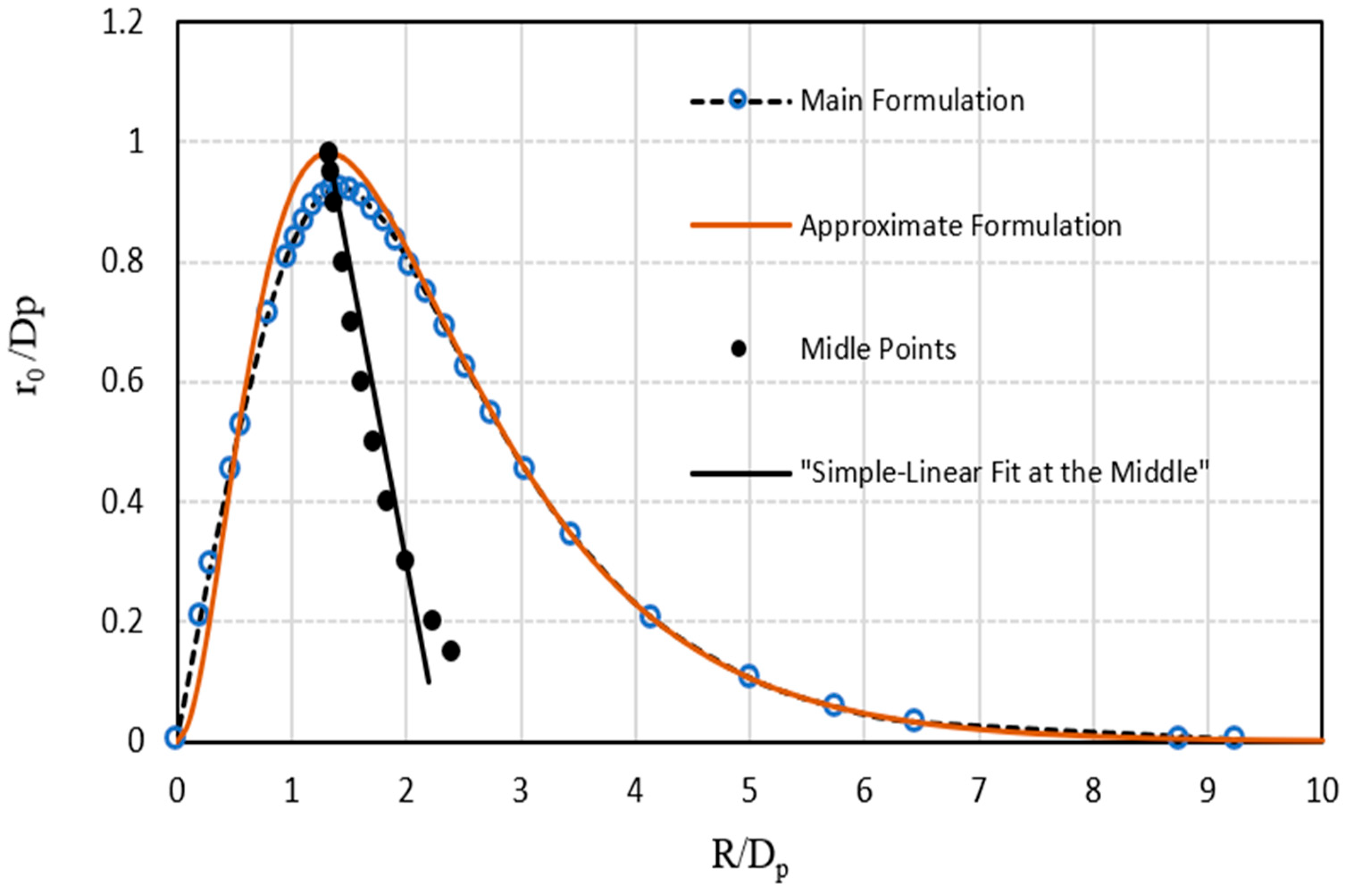
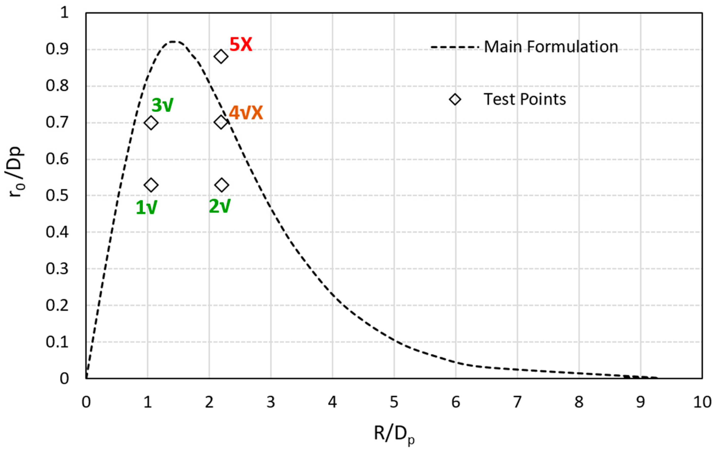
- Analytical results reveal the region for the plausible object size formation in accordance with the Dp and the vial size, bounded by a bell-shaped curve. A particular point of interest is the extremum point on the curve, indicating the maximum possible size of the part that can be produced, regardless of container size, that solely depends on Dp. For uniform light distribution, the ratio of the maximum part size to Dp is 0.92. This is based on the competition for curing between the central regions and the regions adjacent to the inner surface of the vial.
- According to the analysis and the limit curve, for any desirable size of the object (r0), there is a wide selection of vial sizes (R) that can be selected. The smaller the object size, the wider the selection spectrum for the vial size. The actual sizes are governed by the value of Dp, which is the principal criterion for the design of the process.
- A limit graph for the vial diameter showing lower and upper boundaries is introduced by the analytical results. The upper boundary is more important for the selection of the vial diameter for a desired part size. It highlights three criteria for the selection of vial diameter—Single Value, Mid-Point, and Max-Limit.
- A set of experiments was conducted to evaluate the analytical results. The experimental results strongly support the experimental outcomes, affirming the reliability of the analytical evaluation.
Author Contributions
Funding
Data Availability Statement
Conflicts of Interest
References
- Loterie, D.; Delrot, P.; Moser, C. High-resolution tomographic volumetric additive manufacturing. Nat. Commun. 2020, 11, 852. [Google Scholar] [CrossRef] [PubMed]
- Kelly, B.E.; Bhattacharya, I.; Heidari, H.; Shusteff, M.; Spadaccini, C.M.; Taylor, H.K. Volumetric additive manufacturing via tomographic reconstruction. Science 2019, 363, 1075–1079. [Google Scholar] [CrossRef]
- Bhattacharya, I.; Toombs, J.; Taylor, H. High fidelity volumetric additive manufacturing. Addit. Manuf. 2021, 47, 102299. [Google Scholar] [CrossRef]
- Bernal, P.N.; Bouwmeester, M.; Madrid-Wolff, J.; Falandt, M.; Florczak, S.; Rodriguez, N.G.; Li, Y.; Größbacher, G.; Samsom, R.A.; van Wolferen, M. Volumetric bioprinting of organoids and optically tuned hydrogels to build liver-like metabolic biofactories. Adv. Mater. 2022, 34, 2110054. [Google Scholar] [CrossRef]
- Shusteff, M.; Browar, A.E.; Kelly, B.E.; Henriksson, J.; Weisgraber, T.H.; Panas, R.M.; Fang, N.X.; Spadaccini, C.M. One-step volumetric additive manufacturing of complex polymer structures. Sci. Adv. 2017, 3, eaao5496. [Google Scholar] [CrossRef]
- Whyte, D.J.; Doeven, E.H.; Sutti, A.; Kouzani, A.Z.; Adams, S.D. Volumetric additive manufacturing: A new frontier in layer-less 3D printing. Addit. Manuf. 2024, 84, 104094. [Google Scholar] [CrossRef]
- Van Der Laan, H.L.; Burns, M.A.; Scott, T.F. Volumetric photopolymerization confinement through dual-wavelength photoinitiation and photoinhibition. ACS Macro Lett. 2019, 8, 899–904. [Google Scholar] [CrossRef]
- Jacobs, P.F. Rapid Prototyping & Manufacturing: Fundamentals of Stereolithography; Society of Manufacturing Engineers: Southfield, MI, USA, 1992. [Google Scholar]
- Kelly, B.E. Volumetric Additive Manufacturing of Arbitrary Three-Dimensional Geometries in Photopolymer Materials. Ph.D. Thesis, University of California, Berkeley, CA, USA, 2018. [Google Scholar]
- Melchels, F.P.W.; Feijen, J.; Grijpma, D.W. A review on stereolithography and its applications in biomedical engineering. Biomaterials 2010, 31, 6121–6130. [Google Scholar] [CrossRef]
- Riffe, M.B.; Davidson, M.D.; Seymour, G.; Dhand, A.P.; Cooke, M.E.; Zlotnick, H.M.; McLeod, R.R.; Burdick, J.A. Multi-Material Volumetric Additive Manufacturing of Hydrogels using Gelatin as a Sacrificial Network and 3D Suspension Bath. Adv. Mater. Addit. Manuf. 2024, 36, 2309026. [Google Scholar] [CrossRef]
- Orth, A.; Webber, D.; Zhang, Y.; Sampson, K.L.; de Haan, H.W.; Lacelle, T.; Lam, R.; Solis, D.; Dayanandan, S.; Waddell, T.; et al. Deconvolution volumetric additive manufacturing. Nat. Commun. 2023, 14, 4412. [Google Scholar] [CrossRef]
- Toombs, J.T.; Luitz, M.; Cook, C.C.; Jenne, S.; Li, C.C.; Rapp, B.E.; Kotz-Helmer, F.; Taylor, H.K. Volumetric additive manufacturing of silica glass with microscale computed axial lithography. Science 2022, 376, 308–312. [Google Scholar] [CrossRef]
- Rackson, C.M.; Champley, K.M.; Toombs, J.T.; Fong, E.J.; Bansal, V.; Taylor, H.K.; Shusteff, M.; McLeod, R.R. Object-space optimization of tomographic reconstructions for additive manufacturing. Addit. Manuf. 2021, 48, 102367. [Google Scholar] [CrossRef]
- Chen, T.; Li, H.; Liu, X. Statistical iterative pattern generation in volumetric additive manufacturing based on ML-EM. Opt. Commun. 2023, 537, 129448. [Google Scholar] [CrossRef]
- Salajeghe, R.; Meile, D.H.; Kruse, C.S.; Marla, D.; Spangenberg, J. Numerical modeling of part sedimentation during volumetric additive manufacturing. Addit. Manuf. 2023, 66, 103459. [Google Scholar] [CrossRef]
- Orth, A.; Sampson, K.L.; Zhang, Y.; Ting, K.; van Egmond, D.A.; Laqua, K.; Lacelle, T.; Webber, D.; Fatehi, D.; Boisvert, J. On-the-fly 3D metrology of volumetric additive manufacturing. Addit. Manuf. 2022, 56, 102869. [Google Scholar] [CrossRef]
- Regehly, M.; Garmshausen, Y.; Reuter, M.; König, N.F.; Israel, E.; Kelly, D.P.; Chou, C.-Y.; Koch, K.; Asfari, B.; Hecht, S. Xolography for linear volumetric 3D printing. Nature 2020, 588, 620–624. [Google Scholar] [CrossRef]
- Pazhamannil, R.; Hadidi, H.; Puthumana, G. Development of a low-cost volumetric additive manufacturing printer using less viscous commercial resins. Polym. Eng. Sci. 2022, 63, 65–77. [Google Scholar] [CrossRef]
- Madrid-Wolff, J.; Toombs, J.; Rizzo, R.; Bernal, P.N.; Porcincula, D.; Walton, R.; Wang, B.; Kotz-Helmer, F.; Yang, Y.; Kaplan, D. A review of materials used in tomographic volumetric additive manufacturing. MRS Commun. 2023, 13, 764–785. [Google Scholar] [CrossRef]
- Štaffová, M.; Ondreáš, F.; Svatík, J.; Zbončák, M.; Jančář, J.; Lepcio, P. 3D printing and post-curing optimization of photopolymerized structures: Basic concepts and effective tools for improved thermomechanical properties. Polym. Test. 2022, 108, 107499. [Google Scholar] [CrossRef]
- Bagheri Saed, A.; Behravesh, A.H.; Hasannia, S.; Alavinasab Ardebili, S.A.; Akhoundi, B.; Pourghayoumi, M. Functionalized poly l-lactic acid synthesis and optimization of process parameters for 3D printing of porous scaffolds via digital light processing (DLP) method. J. Manuf. Process. 2020, 56, 550–561. [Google Scholar] [CrossRef]
- Bennett, J. Measuring UV curing parameters of commercial photopolymers used in additive manufacturing. Addit. Manuf. 2017, 18, 203–212. [Google Scholar] [CrossRef] [PubMed]
- Gibson, I.; Rosen, D.; Stucker, B. Vat Photopolymerization Processes. In Additive Manufacturing Technologies: 3D Printing, Rapid Prototyping, and Direct Digital Manufacturing; Springer: New York, NY, USA, 2015; pp. 63–106. [Google Scholar]
- Chivate, A.; Zhou, C. Enhanced schlieren system for in situ observation of dynamic light–resin interactions in projection-based stereolithography process. J. Manuf. Sci. Eng. 2023, 145, 081005. [Google Scholar] [CrossRef]


| r0/Dp [r0 (mm)] | R/Dp [R (mm)] |
|---|---|
| 0.53 [3] 0.70 [4] 0.88 [5] (outside the limit) | 1.05 [6] 2.2 [12.5] |
| Exp# | Projected Diameter (mm) | Test Time (s) |
|---|---|---|
| 1 | 2 | 60 |
| 2 | 2 | 90 |
| 3 | 2 | 120 |
| 4 | 2 | 150 |
| 5 | 2 | 180 |
| 6 | 4 | 50 |
| 7 | 4 | 70 |
| 8 | 4 | 90 |
| 9 | 6 | 50 |
| 10 | 6 | 60 |
| Vial Internal Diameter | Projected Diameter | Curing Inside Vial | Produced Object |
|---|---|---|---|
| 12 mm | 6 mm (r0 = 3 mm) (Point 1) |  At 16 s | 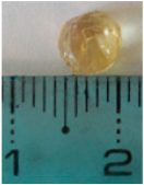 6.1 mm Dia |
| 8 mm (r0 = 4 mm) (Point 3) | 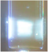 At 16 s | 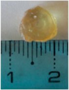 8.3 mm Dia | |
| 25 mm | 6 mm (r0 = 3 mm) (Point 2) | 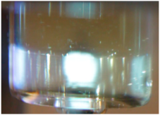 At 50 s |  6.3 mm Dia |
| 8 mm (r0 = 4 mm) (Point 4) | 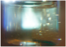 At 50 s | 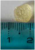 8.5 mm Dia with gel | |
| 10 mm (r0 = 5 mm) (Point 5) |  At 45 s | No object was produced due to a lot of surface curing |
| Projected Diameter | Curing Inside Vial and Part Produced | |
|---|---|---|
| 2 mm (r0 = 1 mm) |  At 60 s 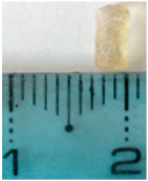 2.9 mm Dia | 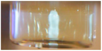 At 150 s  3.8 mm Dia |
| 4 mm (r0 = 2 mm) | 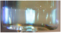 At 70 s 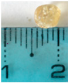 4.4 mm Dia | 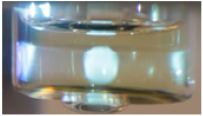 At 90 s  4.7 mm Dia |
| 6 mm (r0 = 3 mm) | 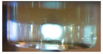 At 50 s 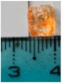 6.3 mm Dia | |
Disclaimer/Publisher’s Note: The statements, opinions and data contained in all publications are solely those of the individual author(s) and contributor(s) and not of MDPI and/or the editor(s). MDPI and/or the editor(s) disclaim responsibility for any injury to people or property resulting from any ideas, methods, instructions or products referred to in the content. |
© 2025 by the authors. Licensee MDPI, Basel, Switzerland. This article is an open access article distributed under the terms and conditions of the Creative Commons Attribution (CC BY) license (https://creativecommons.org/licenses/by/4.0/).
Share and Cite
Behravesh, A.H.; Tariq, A.; Buni, J.; Rizvi, G. Computed Tomography-Based Volumetric Additive Manufacturing: Development of a Model Based on Resin Properties and Part Size Interrelationship—Part I. J. Manuf. Mater. Process. 2025, 9, 178. https://doi.org/10.3390/jmmp9060178
Behravesh AH, Tariq A, Buni J, Rizvi G. Computed Tomography-Based Volumetric Additive Manufacturing: Development of a Model Based on Resin Properties and Part Size Interrelationship—Part I. Journal of Manufacturing and Materials Processing. 2025; 9(6):178. https://doi.org/10.3390/jmmp9060178
Chicago/Turabian StyleBehravesh, Amir H., Asra Tariq, John Buni, and Ghaus Rizvi. 2025. "Computed Tomography-Based Volumetric Additive Manufacturing: Development of a Model Based on Resin Properties and Part Size Interrelationship—Part I" Journal of Manufacturing and Materials Processing 9, no. 6: 178. https://doi.org/10.3390/jmmp9060178
APA StyleBehravesh, A. H., Tariq, A., Buni, J., & Rizvi, G. (2025). Computed Tomography-Based Volumetric Additive Manufacturing: Development of a Model Based on Resin Properties and Part Size Interrelationship—Part I. Journal of Manufacturing and Materials Processing, 9(6), 178. https://doi.org/10.3390/jmmp9060178