Investigation of the Thermo-Mechanical Modeling of the Manufacturing of Large-Scale Wire Arc Additive Manufacturing Components with an Outlook Towards Industrial Applications

Abstract

The simulation of additive manufacturing processes, such as Wire Arc Additive Manufacturing (WAAM), is becoming increasingly important to predict material and component properties in advance of the real-life manufacturing. In contrast to prior work focusing on the simulation of simplified WAAM parts, this paper presents an investigation into the thermo-mechanical finite element (FE) simulation of the manufacturing of large-scale WAAM components. The investigation focuses on various problems within the individual steps of the FE workflow wherein ABAQUS influences the modeling of large-scale components. The investigations are founded upon a thermo-mechanically coupled FE model in ABAQUS 2020. For this purpose, several thermo-mechanical simulation models are set up with the target of investigating the meshing, element activation and variation of process parameters. Appropriate discretization of WAAM components is found to be a major problem when setting up a simulation. The meshing of the component is limited by the element type and size and the meshing routines used. Also, differences in the axes of motion for the simulation and the real process cause the simulation to differ from reality. High element start temperatures are found to be beneficial for simulation stability and performance. An integrated parameter variation was made possible with the modeling techniques used.

1. Introduction

In the context of global supply chains and with consideration for a resource-efficient economy, additive manufacturing is becoming increasingly relevant as a process for manufacturing metallic components. An illustration of this development can be found in the increasing reliance on third-party countries for the supply of casted parts caused by the ongoing reduction in production capacities within the German steel foundry sector [1]. Additive manufacturing processes, such as Wire Arc Additive Manufacturing (WAAM), have the potential to contribute to the maintenance of production capacity through flexible production planning and short throughput times.

The WAAM process is predicated on the functional principles of classic welding processes such as metal inert gas welding (MIG), metal active gas welding (MAG) and tungsten inert gas (TIG) welding. In these processes, material in the form of a standard welding wire is melted by a plasma arc and then transferred to the workpiece as a liquid droplet. The generation of the plasma arc is facilitated by applying a voltage between the workpiece and the welding torch. In the case of the MIG/MAG process, the voltage is generated between the welding wire and the workpiece. The generated voltage causes ionization of the surrounding gas, leading to the formation of plasma in this area. The resultant heat enables temperatures to be achieved in the range of several thousand degrees Celsius [2].

In additive manufacturing, the deposition of material is carried out layer by layer to achieve a certain geometry. For WAAM, the melting of the welding wire is used to deposit the material in each layer. The implementation of path movements is typically accomplished through the use of an industrial robot or gantry portal machines. Compared to other additive manufacturing processes for metallic materials, WAAM is distinguished by its high deposition rates and low system costs. It can be used to manufacture components that would otherwise be produced using a combination of casting, forging and milling. The greatest potential for WAAM lies in the fast and resource-saving production of large-volume components for the energy generation, heavy industry and aerospace sectors. In the context of utilizing WAAM for the fabrication of safety-critical components, such as those employed in nuclear facilities, there exist specific regulations with regard to the component properties. Suitable and comprehensive measures for evaluation and quality assurance are required [3]. Here, experimental methods such as non-destructive testing and mechanical material testing can be employed to identify defects in components [4]. However, these methods are usually associated with expensive testing equipment or complex sample preparation that requires the component to be destroyed [4].

The increasing computing power of modern processors offers a further opportunity for the evaluation of manufacturing processes in general. Examples of the use of manufacturing simulation can be found for almost all modern manufacturing processes. For example, Huang et al. [5] used finite element (FE) simulation to model the cutting edge of a tool for machining metal components in order to find advantageous tool geometries. This contributed to the productivity of different machining processes using this kind of tools. A different approach, by Almonti et al. [6], uses an FE analysis to validate the results of experimental thermography measurements. This combination is intended to improve the thermal diffusion of metal matrix components in coating technology. For the process of WAAM, simulation offers the prediction of component properties, including microstructure and residual stresses, prior to the commencement of production. This means that the time-consuming process of experimentally recording properties is reduced, or even rendered entirely needless [7]. Furthermore, the simulation facilitates the exploration of process parameters, enabling the determination of the most optimal parameters for subsequent manufacturing processes. Also, the need for experimental testing can be significantly reduced.

1.1. Simulation of Additive Manufacturing

As is the case with the majority of additive manufacturing processes for metallic materials, WAAM is also associated with a high localized heat input. Consequently, this results in the occurrence of exceedingly high heating and cooling rates, which are accompanied by thermal expansion during the heating process and thermal contraction during the cooling process. It is important to note that the thermally induced strains can lead to considerable residual stresses and a large distortion of the component. In this context, residual stresses manifest themselves in particular in areas that impede the strains from the expanding material. In addition to thermally induced strains, high heating and cooling rates, analogous to those employed in conventional fusion welding processes, exert a substantial influence on the material microstructure within the weld bead area. In the region designated as the heat-affected zone (HAZ), diverse microstructure types are formed [8] which vary in their properties (e.g., in terms of strength or toughness) depending on the temperature, the time and the cooling rate. The formation of microstructures in welding processes with a single welding layer can be estimated with reasonable ease by measuring the temperature. However, as the number of welding layers increases, the complexity of the process significantly increases, as the newly applied bead and previously welded beads are influenced by the process heat. These phenomena already manifest themselves in simple geometries, such as bars, beams or plates, and can be easily analyzed. Their quantification can be achieved through the utilization of analytical equations or by experimental determination. However, for more complex geometries with numerous welded layers, a common occurrence in many instances of additive manufacturing, this approach becomes untenable. Experimental methods, too, are limited in their capacity to provide meaningful results in such cases due to the extended production times and costs that are required for large components, which precludes the possibility of extensive parameter variation.

The complexity of additive manufacturing processes, characterized by a multitude of relevant parameters, further complicates the prediction of outcomes. However, modeling on a microscopic level offers the possibility of making quantitative predictions about the microstructure and its properties in additively manufactured components [7]. In this context, numerical approaches such as the phase-field model [9,10] or the kinetic Monte Carlo Potts model [11] are used for modeling the microstructure formation. In addition to the spatial formation of the microstructure, the interaction of individual microstructural components can be combined to simulate the microstructural properties. The individual structural components are modeled using the FE method in order to determine the overall mechanical state of the microstructure in combination with the respective mechanical properties [12]. Conversely, modeling at the macroscopic level is more concerned with the process-related thermal and mechanical reactions at the component level. In order to model the processes during the course of additive manufacturing, it is possible to carry out process and structure modeling as a thermal, mechanical or thermo-mechanically coupled simulation [13]. In all of these variants, adequate modeling of the heat input and the additive material deposition is crucial for correctly representing the process. Numerical methods can be employed to achieve this. Notable examples of such methods include FE simulations [14,15] and computational fluid dynamics (CFD) simulations [16,17]. While FE simulations are predominantly employed in the modeling of thermo-mechanical processes, CFD simulations have the capacity to depict fluid processes within the melt pool [7].

1.2. Simulation of WAAM

As previously stated, WAAM processes demonstrate their process-related advantages, particularly in the context of large-scale components. The dimensions of the individual weld beads utilized in the component’s construction can differ considerably from its overall size, with the discrepancy potentially extending to several orders of magnitude. In the simulation of WAAM, this discrepancy gives rise to a conflict in the geometric resolution of the component to be simulated. The objective is to be able to have a realistic exemplar component (i.e., large and complex) that can be modeled as completely as possible. In order to ensure that the calculation is efficient in terms of the resources employed, it is necessary to design the mesh within the FE calculation in a relatively coarse manner, i.e., with large elements. The use of an excessive number of elements can impede the feasibility of conducting the FE calculation within a reasonable time frame, particularly in scenarios where no high-performance computing is employed. A further possible objective of the calculations is to model the heat input into the material as accurately as possible during material deposition. To achieve this, it is imperative that the distribution of the power density within the heat source can be resolved over a sufficient number of elements. In this regard, the choice of element size is pivotal, with smaller elements leading to more accurate power distribution mapping. It is imperative to assess which variables are instrumental in determining the simulation outcome and to what extent simplifications can be employed. One such approach involves reducing the dimensions of the simulation, as demonstrated by Mughal et al. [18]. In this approach, a two-dimensional simulation is conducted, wherein a section of a component is meshed with two-dimensional elements. In [14,19,20,21,22,23], simplification is achieved through the simulation of highly simplified geometries. The simulations carried out in these studies illustrate the configuration of a wall composed of individual weld beads that are superimposed. This approach facilitates the clear visualization of the heat source and enables fundamental parameter studies to be conducted. A similar approach can be found in the publications by Mughal et al. [24], Zhao et al. [25] and Amal et al. [26]. In these cases, the complexity is reduced to a single layer of a component. The focus of the simulations in these cases is on the influence of different path planning strategies on warpage and residual stresses. To extend this concept, Chiumenti et al. [27] and Israr et al. [28] created cuboids consisting of several layers to visualize the simulation of a real component. However, both works are still far from the scale of a real WAAM-manufactured component, with 14 layers and 22 mm height [28] and 40 layers and 50 mm height [27], respectively. The simulation of a simple tube structure by [22,29,30] marked a significant step towards the creation of realistic components. In each of these studies, the tube was constructed with a wall thickness corresponding to the weld bead width. The tube lengths in these works varies from 16 mm [30] to 60 mm [29].

1.3. Motivation and Objectives

However, it can be seen that, in most cases, the geometries analyzed only correspond to a small extent to the components that can be produced particularly efficiently with WAAM. Despite endeavors to implement larger structures to enhance their resemblance to reality, these structures are also of a different order of magnitude. Further, only geometries without complex meshing requirements were used in the discussed publications. In the extant literature, the limitation of computing capacity is cited as the reason for the reduction in the simulated component size [31], but further investigations have revealed additional limitations. In order to enhance the simulation of large-volume components, it is necessary to identify and address the existing limitations within this order of magnitude. This paper presents an investigation into the thermo-mechanical FE simulation of larger and more complex component geometries. The investigation focuses on the individual steps of the classic FE workflow, wherein ABAQUS and its associated routines are employed for the simulation of additive manufacturing. These include the meshing of the component, the application of boundary conditions, the realization of the path movement and the modeling of geometric structures. In addition to computing capacity, these factors significantly influence the possibilities for simulating large-volume components and should therefore be taken into account when designing a model.

2. Materials and Methods

In this study, a range of influencing variables is analyzed with the aim of developing a more profound understanding of the simulation of large-scale WAAM components. The investigations are based on an ABAQUS simulation model that was created using the integrated ‘AM Modeler’ plug-in. This plug-in integrates subroutines into the ABAQUS CAE user interface, facilitating the implementation of element activation and a heat source. The subsequent sections describe the finite element model configuration with respect to the simulation approach, the boundary conditions and the material model employed.

2.1. Modeling Approach

The investigations are founded upon a thermo-mechanically coupled finite element model in ABAQUS 2020. The calculation of the thermal and mechanical model parts is coupled sequentially. Initially, thermal variables are calculated due to the influence of the heat source, which subsequently serve as input variables for the mechanical calculation. The activation of the elements of the FE model for modeling the material deposition is carried out using the ‘inactive elements’ approach, also known as the ‘element birth and death’ technique [19]. This approach involves the deactivation of all elements of the model at the start of the calculation that are later identified as constituting the geometry of the additively manufactured component. During the simulation, these elements are reactivated by the ’bead’ function of the AM Modeler, depending on the path planning. It is important to note that, when deactivated, these elements exert no influence on the thermal or mechanical behavior of the model. A common heat source model according to Goldak et al. [32] is utilized in all investigations to model the heat input from the molten pool and the arc. The three-dimensional heat source has a double ellipsoidal shape, located below the surface of the material, and has different power densities before and after the center of the heat source (see Figure 1). The mathematical description of the power density q of the front and rear ellipsoids is achieved through the utilization of Equation (1) for the front part of the ellipsoid and (2) for the rear part, respectively, contingent upon the specific spatial position.

Figure 1. Double ellipsoid Goldak heat source model [32].

Figure 1. Double ellipsoid Goldak heat source model [32].

$$q(x,y,z)={\displaystyle \frac{6\sqrt{3}{f}_{f}Q}{ab{c}_f\pi \sqrt{\pi }}}{e}^{\left[-3\left({\displaystyle \frac{x^2}{c_f}}+{\displaystyle \frac{y^2}{a^2}}+{\displaystyle \frac{z^2}{b^2}}\right)\right]}$$

(1)

$$q(x,y,z)={\displaystyle \frac{6\sqrt{3}{f}_{r}Q}{ab{c}_r\pi \sqrt{\pi }}}{e}^{\left[-3\left({\displaystyle \frac{x^2}{c_r}}+{\displaystyle \frac{y^2}{a^2}}+{\displaystyle \frac{z^2}{b^2}}\right)\right]}$$

(2)

Equations (1) and (2) define two three-dimensional half ellipsoids. These are based on half of the width of the heat source a, the depth of the heat source b and the front and rear ellipsoid lengths $c_f$ and $c_r$. The existing power via the plasma arc is introduced into the equations through the welding power Q and the proportional power in the front and rear part of the heat source $f_f$ and $f_r$. According to Equation (3), the welding power in arc welding is the result of the thermal efficiency of the arc ($\eta$), the welding voltage (U) and the welding current (I) [29]. The factors $f_f$ and $f_r$, which represent the division of the welding power between the front and rear ellipsoids, must collectively equal 2, as defined by Goldak et al. [32] in Equation (4).

$$Q=\eta IU$$

(3)

$$f_f+f_r=2$$

(4)

The implementation of the movement of the heat source and bead for element activation requires the AM Modeler to list points in a table, which are traversed one after the other. This procedure bears a resemblance to that of CNC-controlled manufacturing processes. The AM functions of Siemens NX are utilized for the fundamental creation of path planning in g-code format. Subsequently, the information on the movement of the path is added in a specially programmed conversion tool, and temporal information is added to also take travel speeds into account. Furthermore, the data tables are augmented by the power of the welding source and information concerning the material deposition.

For the thermal simulations, brick elements of type DC3D8 and tetrahedron elements of type DC3D8 are used. The mechanical calculations are carried out with C3D8R brick elements with reduced integration and with C3D10 tetrahedron elements. Further element controls are left at the default settings of ABAQUS. The elements used are described in each simulation example if relevant.

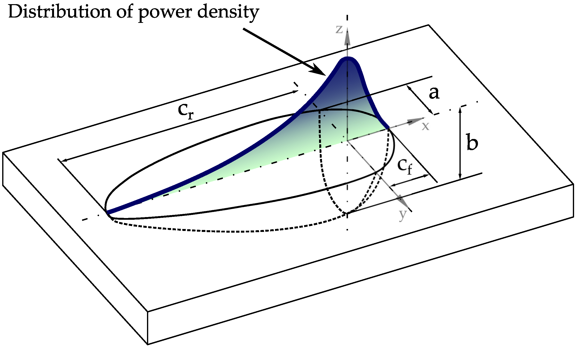
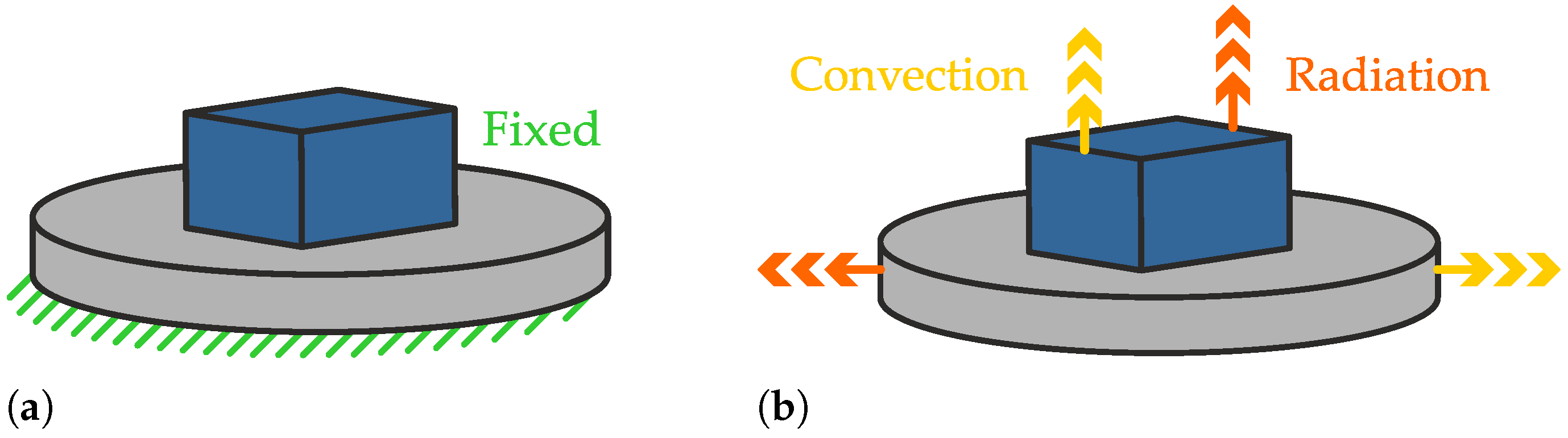
2.2. Boundary Conditions

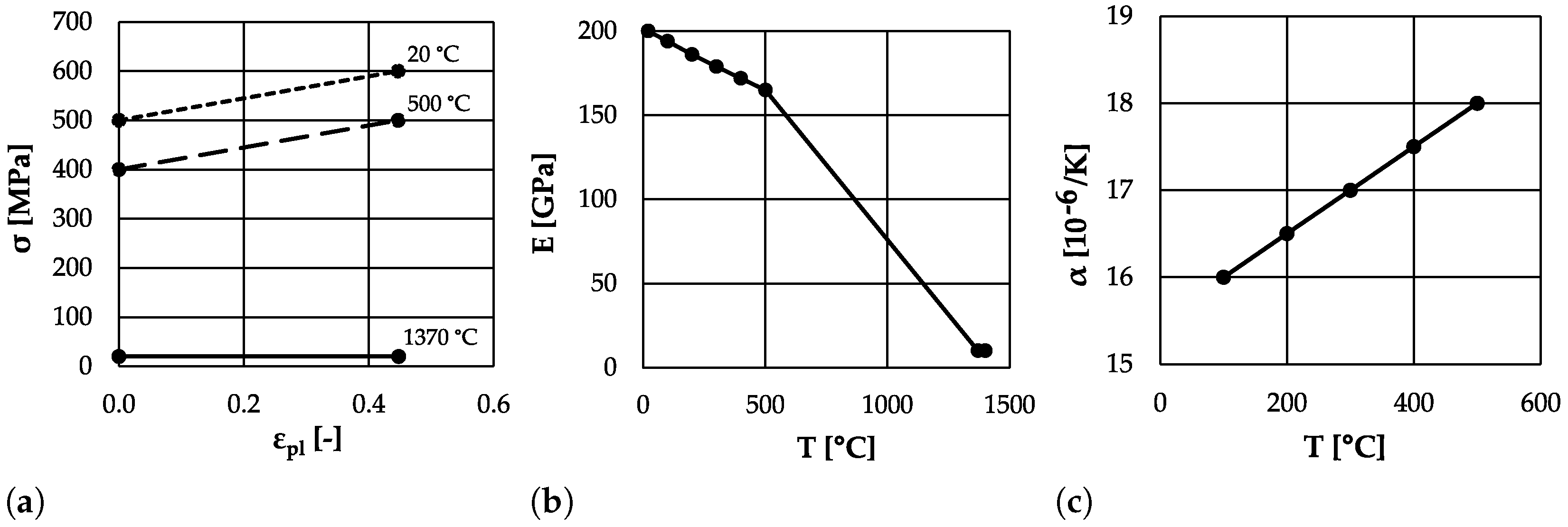
All structures applied additively as part of the simulation are subject to the same boundary conditions. As illustrated in the figure below, the deposition of material (blue) is executed on a base plate (gray). This base plate is firmly clamped against displacement and torsion in all spatial directions on its lower surface (see Figure 2a). With respect to thermal boundary conditions, all active element surfaces exhibit a convection and radiation boundary condition, facilitating heat transfer to the environment (see Figure 2b).

Various reference values for the emissivity of radiation and the heat transfer coefficient of convection can be found in the literature. Baehr et al. [33] used numerical values in a range between 0.446 and 0.488 for the emissivity of sandblasted steel, while Kuchling et al. [34] assumed values between 3.5 and 35 ${\displaystyle \frac{W}{m^{2}K}}$ for the heat transfer coefficient from air to a metal wall. Although these two conditions do not correspond exactly to those in WAAM, they can be used for simplification. An emissivity of 0.4 for radiation and a heat transfer coefficient of 20 ${\displaystyle \frac{W}{m^{2}K}}$ for convection are assumed as parameters for the simulation model. The ambient temperature for radiation and convection is 26 °C in all models.

In both the thermal and mechanical calculations, all elements of the model are assigned a starting temperature. The elements of the base plate are initially given a temperature of 26 °C, while the elements of the additively manufactured component are activated at a temperature of 26 or 1400 °C, depending on the investigation. The given temperatures are the same for the thermal and mechanical parts of the calculations. The temperature used is specified in each respective section if relevant.

2.3. Material

Since this paper does not focus on the results of the simulation, the material model used corresponds to the model used by Käß et al. [15] for 316L steel and is adapted for this work. The results of this work are not influenced by the material model used.

Table 1. Temperature-independent material properties of the 316L material model.

Parameter	Value	Unit
Thermal conductivity	16.2	${\displaystyle \frac{\mathrm{W}}{\mathrm{mK}}}$
Specific heat capacity	500	${\displaystyle \frac{\mathrm{J}}{\mathrm{kgK}}}$
Specific melting heat	270,000	${\displaystyle \frac{\mathrm{J}}{\mathrm{kg}}}$
Solidus temperature	1644.15	K
Liquidus temperature	1673.15	K
Density	7900	${\displaystyle \frac{\mathrm{kg}}{{\mathrm{m}}^3}}$
Poisson’s ratio	0.3	-

shows the temperature-independent material properties.

Figure 3 shows the temperature-dependent material characteristics of the material model used. Adjusted flow curves, Young’s modulus and the coefficient of thermal expansion are used. Vaporization of the material is not considered in the material model.

3. Numerical Studies

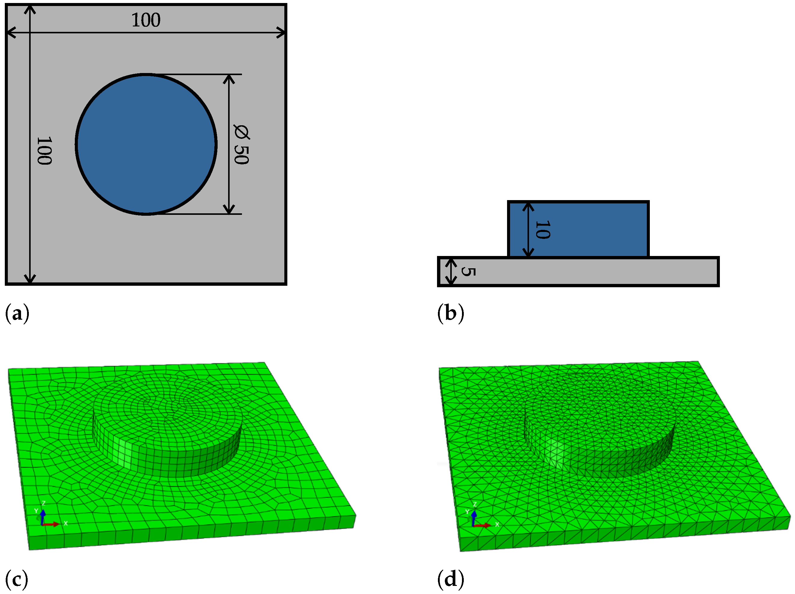
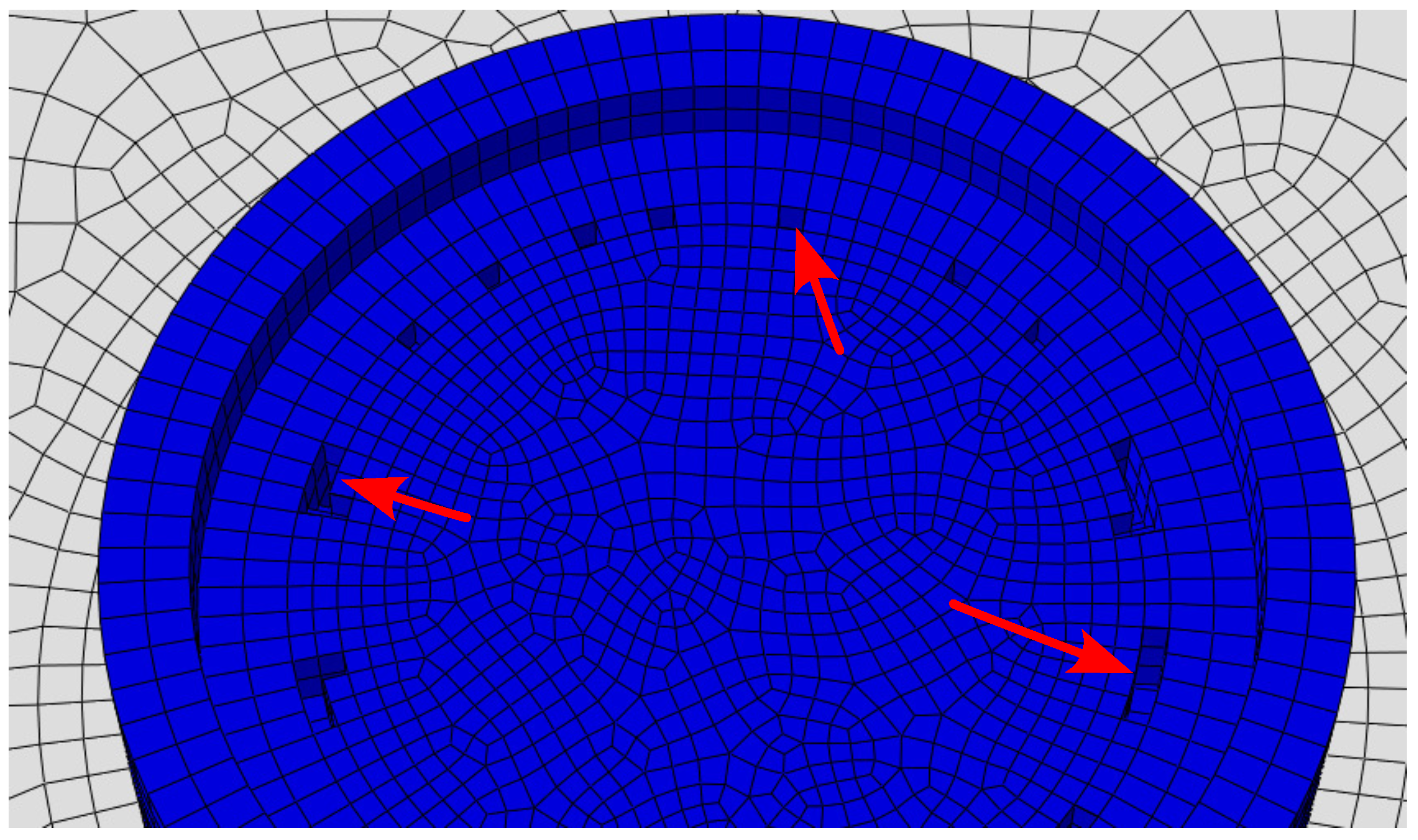
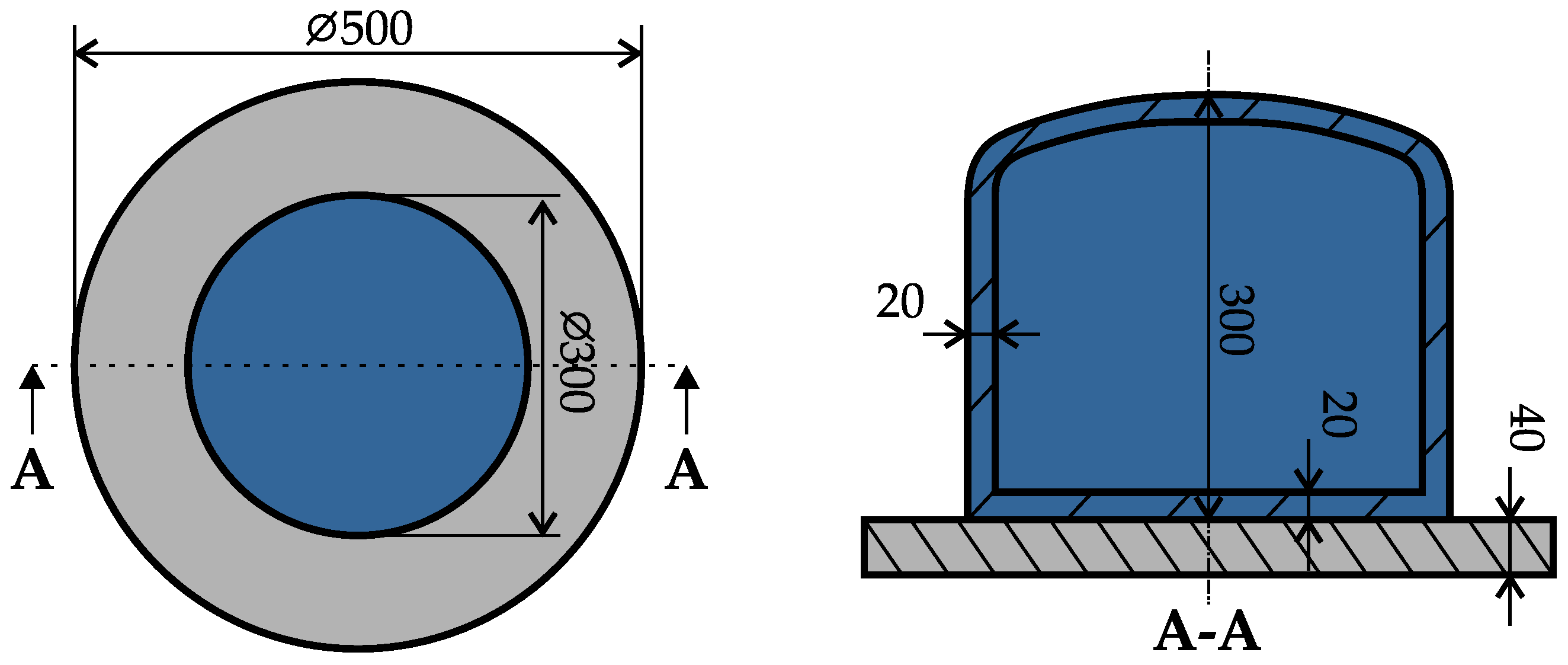
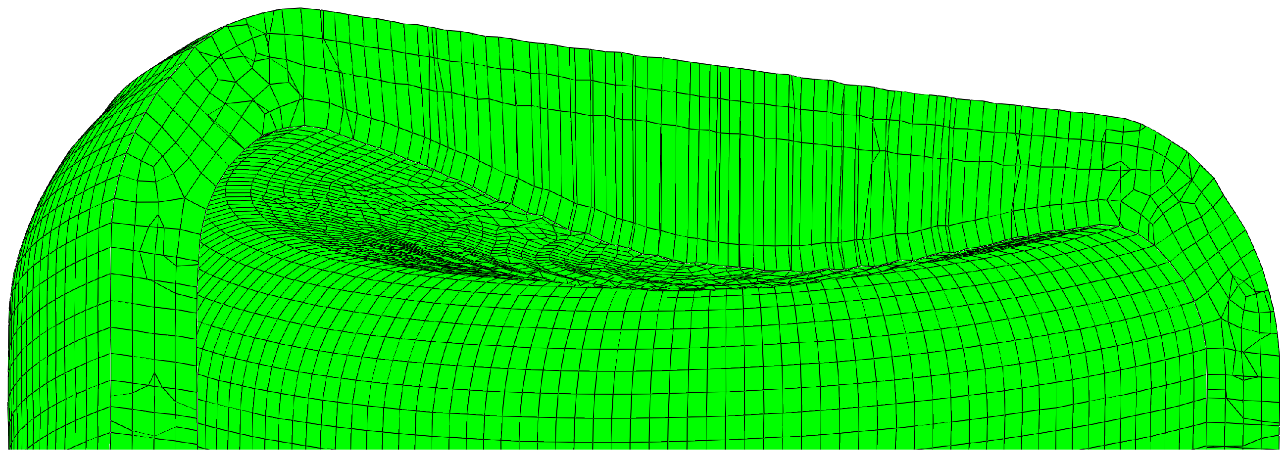
The individual aspects of the simulation of large-scale WAAM components are highlighted below. The topics of meshing, element activation and the representation of process parameters were identified as particularly relevant. Different numerical studies have been carried out on the above-mentioned topics.

3.1. Meshing

The meshing of components for FE simulations is an important basis for generating valid results. The element type, element size and meshing technique are essential elements for creating a high-quality mesh. These points become even more important if the mesh has a decisive influence on the quality of the representation of the process, as in the simulation for WAAM. As discussed in Section 1, previous work on the simulation of WAAM has mainly focused on simple and relatively small geometries. In addition to the limitations of the calculation capacity, limitations in the meshing of the components due to program-specific framework conditions also represent a possible relevant problem. This issue is ignored by using simple geometries, and only a limited prediction about the possibilities for simulating larger and more complex geometries can be made.

• Mesh type:

The element type best suited for meshing components in regular FE calculations is largely determined by the geometry of the component and the necessary accuracy of the calculation. Other relevant influences are not to be expected, as the mesh usually does not change during the calculation with regard to the number of elements. This assumption cannot be made for the simulation of additive manufacturing processes as the elements must be activated and deactivated during the calculation. For a good representation of the WAAM process, it is necessary to clarify which element type is generally best suited for the simulation. In order to decide which element type is best suited, example geometries with hexagonal and tetragonal elements are compared below. For this purpose, two thermo-mechanical simulation models with the same geometry and the same simulation parameters are set up which differ only in the type of element. The component geometry used and the different mesh types investigated are shown in Figure 4.

Regarding the results of the mechanical calculation with tetragonal elements, the element activation in combination with the heat source causes problems when using this type of element. Figure 5 shows the front tip of a weld bead that has just been applied. The area marked in red shows the elements that were activated last. It is noticeable that some elements are only connected to other elements on one of the four side surfaces after activation. One of the element’s nodes floats freely in space. This can be explained by the fact that the elements are activated as soon as they are cut by the bead of the AM Modeler for the first time. If there is then an unfavorable combination of the position of the element and the path planning, such geometries can arise on the weld bead front.

In addition to the problem that this does not correspond to the real geometries of a weld bead, it can also lead to a strong deformation of such elements, as shown in Figure 6, as the node lying freely in space is not connected to the rest of the mesh. This means that its spatial fixation is only determined by the mechanical properties of its own element and is not additionally prevented from moving by adjacent elements. The deformation seen here is more than ten times greater in the simulation than shown in the image. The points mentioned do not allow the use of tetragonal elements in combination with the AM Modeler and the element activation stored there for the WAAM process. Such phenomena cannot be observed in the results of the calculations with hexagonal elements.

• Mesh size:

Due to the fact that individual elements must be activated for the material deposition with the AM Modeler, the element size is directly related to the size of the weld bead applied. Regarding the deposition of a weld bead, only elements that lie within the volume of the weld bead should be activated in order to realistically model the welding process. If an activated element lies completely or partially outside the weld bead, too much material volume is activated and the process is not mapped with the correct layer height or weld bead width. To illustrate this, Figure 7 shows three different element sizes for meshing the same weld bead geometry. The target geometry of the weld bead is highlighted in green, the bead of the AM Modeler in red and the elements used in blue.

On the far left, the element size corresponds exactly to the size of the bead. This means that the bead height and width match the element height and width. When meshing in this way, only the exact amount of material volume contained in the desired weld bead is activated. If the weld bead is to be mapped more precisely, the element width can be halved, for example, as shown in the middle of the image, in order to have two elements across the bead width instead of just one. The same is made possible by halving the element height. However, if an increase in the size of the elements is desired due to excessive computing time caused by large components or high temporal resolution, this results in restrictions in the maximum element size. If, for example, the element height is increased to a value greater than the bead height, as in the right-hand part of Figure 7, the activation of the large element results in an excess material volume being activated. In this case, the desired layer height of the simulation is no longer maintained. As a result, the real values of the maximum element size are bound to the geometry of the weld bead, as already described, which means that the lowest possible spatial resolution of a simulation of WAAM is also given by this geometry. Since the geometry of the weld bead should be based on real processes, it cannot be freely selected to allow larger elements. If the spatial resolution is to be further reduced, this can only be achieved by applying several weld bead layers simultaneously.

• Meshing technique:

Knowledge about which component geometries can be simulated at all offers great added value for estimating the capacities of the model for WAAM. For this reason, various component geometries are examined here in the meshing phase in order to verify meshing with hexagonal elements as far as possible.

Two main techniques are available in ABAQUS for meshing with hexagonal elements. Components can be meshed using either the ‘Structured’ or the ‘Sweep’ technique. However, not all geometries can be meshed using both techniques. The ‘Structured’ function is primarily designed for simple and regular geometries and ensures evenly distributed elements of approximately the same size. However, if the geometry becomes more complex, either ‘Structured’ meshing can no longer be used at all or so-called ‘partitions’ must be created on the component. The ‘partitions’ are used to divide the complex component into simpler geometries, which can then be meshed using the “Structured” method. Figure 8 shows an example of partitioning a hollow cylinder and the resulting mesh.

The lines shown there indicate the levels at which the component is divided. For example, the round structure of the cylinder is divided into quarter circles and into individual layers by height. All areas shown in green in the image can be meshed using the “Structured” technique. The area shown in yellow at the top of the lid is not divided and can therefore only be meshed using the Sweep technique. The division of the geometry is completely up to the user of ABAQUS and can, in principle, be as complex as desired. It can be said that a mesh created using the “Structured” technique is better suited for use with the AM Modeler, as the elements created there can be positioned perfectly within a weld bead. If the technique is applied to a thin pipe wall, for example, the result is similar to the meshing of Zhao et al. [29].

To demonstrate what results can be expected with solid round structures, Figure 9 shows another example of two variants for dividing the base of the hollow cylinder. In the left part of the image, the aim of the division is to achieve complete meshing using the “Structured” method. This can only be achieved through a large number of partitions and requires a great deal of effort in the preparation of the 3D model. In most places, the resulting mesh provides good mesh quality in terms of element shape. However, in some places, especially where the split geometry is very pointed, there is a significant reduction in the element size.

With both of the above methods for dividing the component, elements inside the floor are never exactly within the intended weld path and are sometimes also next to it. If the position is unfavorable relative to the path planning of the bead, this can result in elements being activated too early or not at all, as shown in Figure 10.

As can be seen from the previous chapters, path planning and the meshing procedure influence each other to a degree that cannot be ignored. To investigate the interaction, a larger geometry in the style of a pressure vessel is examined in this section. The focus in path planning here is primarily on the production of the cover and its representation by the simulation. At the same time, the extent to which the real process can be modeled using ABAQUS must be examined. In terms of process modeling, the simulation in ABAQUS has major differences compared to the real process, particularly with regard to the number of movement axes. As shown in Figure 11a, the heat source and bead can only be moved in the direction of the three translational axes of a Cartesian coordinate system in the simulation with the AM Modeler in ABAQUS 2020.

The surface of the bead is aligned at each point so that the direction of movement is a normal vector to the bead. Since the bead determines the geometry of the simulated weld bead, its geometry is subject to the same restrictions. The orientation of the heat source is based on the global coordinate system using the equations for the Goldak heat source. The surface of the heat source is always at right angles to the surface of the bead. In comparison, a much freer positioning of the weld bead in relation to the component is possible in the real process (Figure 11b) due to a larger number of movement axes. The use of a robot arm alone means that the welding gun can be positioned over three translational and three rotational axes. If a movable welding table is also used, two additional rotary axes are added, which can be used to position the base plate and the component on it relative to the welding gun. This makes it possible to vary the installation direction of the individual weld bead layers within a single component during the process. For comparison, part of the pressure vessel wall is shown in Figure 12. On the left, it shows the only way in which such a geometry can be implemented with the AM Modeler (ABAQUS 2020). Here, the individual weld beads are activated via the bead, always in the same building direction, and must be shifted horizontally in relation to each other to reproduce the geometry, which is a major flaw of simulating realistic behavior. However, this results in overhangs in the weld beads, particularly in the upper area of the component, which cannot be finished if the real behavior of a weld pool is taken into account. To avoid this problem in the real process, as Figure 12b shows, the building direction along the wall is changed by rotating the component. This means that welding can always take place in the preferred welding position.

In addition to the occurrence of overhangs in the simulation, the described positioning of the bead can lead to problems in element activation for component geometries of this type. To investigate this, the pressure vessel with the dimensions shown in Figure 13 is implemented in an FE calculation. This geometry is inspired by a part possibly used in nuclear applications. The size of the component is an attempt to more closely mirror the dimensions of real components. The lid of the pressure vessel has a permanent curvature up to the central axis with the same wall thickness as the pipe underneath and thus represents an extreme case of the problem described above.

A look at the results of the element activation in Figure 14 reveals exactly the problems described. In Figure 14a, in the transition area from the pipe section to the curvature of the cover, it can be seen that the shape of the four activated elements no longer corresponds to the rectangular shape of the bead. This means that the actual shape of the weld bead is no longer correctly reproduced. In addition, the position of the activated elements creates sharp edges as the surface of the weld bead, which does not correspond to a good representation of the real process. The rotation of the elements is caused by the automated meshing tool, which adapts the position of the elements to the curvature of the component. The problem of freely overhanging elements can be seen in Figure 14b. The AM Modeler activates elements that hang freely in the air by following the path planning.

The reason for this can be found in the activation routines of ABAQUS. These activate the elements layer by layer with a specific offset in the building direction. While this is not a problem in the thermal simulation, it could lead to problems in the mechanical simulation due to the motion of certain elements. As the elements have no fluid dynamic properties and gravity is neglected in the model, there should be no irregularities occurring in the model. However, as can be seen in Figure 15, during the mechanical part of the simulation, a strong deformation of the lid of the pressure vessel can occur. This is introduced only into the second layer of the lid, and the first layer seems to have normal deformation. The reason for this can also be found in the possible simulation design given by ABAQUS 2020. After the first layer of the lid is activated, the activation of the second layer with its implemented expansion and shrinkage introduces great internal stresses into to element beneath. Due to these, plastic deformation is introduced in these regions. This effect reduces with the increase in the activated material volume in the layers above.

In order to achieve a more realistic representation of the cover or the individual weld beads, it would be possible to adapt the geometry to the simulation-specific requirements. However, this is in conflict with the simulation’s representation of real component geometries.

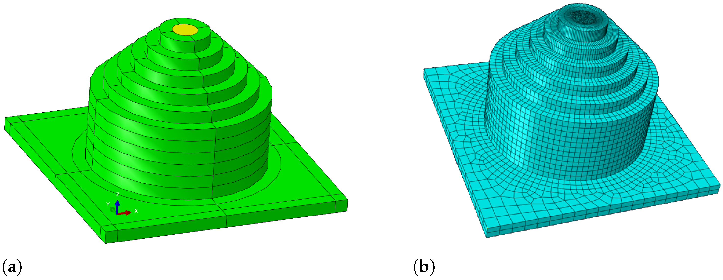
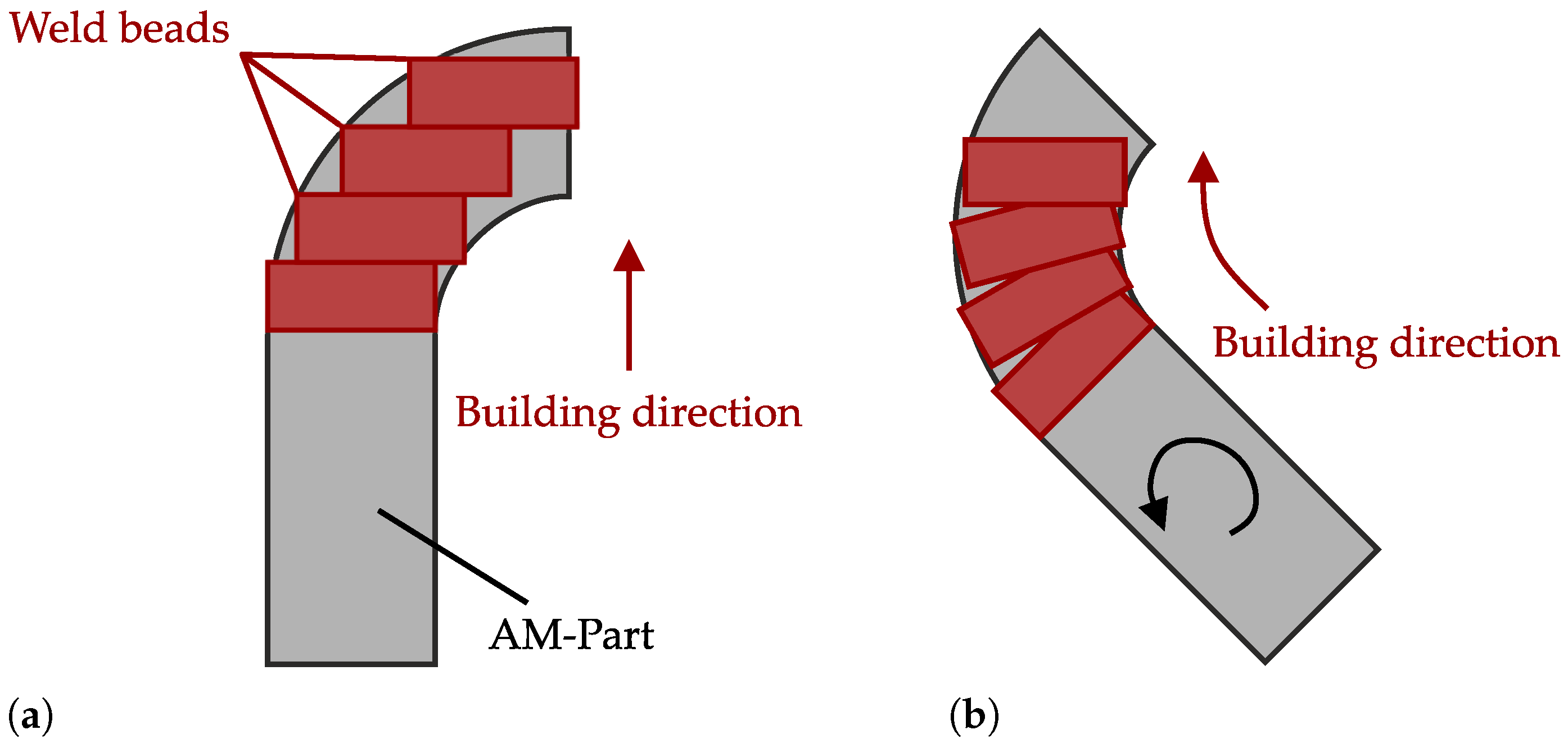
3.2. Element Activation

The elements of the additively manufactured component that are activated by the bead must be assigned a start temperature at the time of activation. This temperature is then influenced within the simulation by the energy of the heat source, the heat conduction within the component and heat transfer to the environment. At this point, the question arises as to which temperature is best suited as the activation temperature for modeling the process.

It is conceivable to use the ambient temperature (here, 26 °C) as the starting temperature of the elements. In this case, the elements are activated in a solid state and then heated above the melting temperature by the heat source. This is similar to the heating of the welding filler material from ambient temperature to melting temperature by the arc in the real process. The input variables welding current, welding voltage and efficiency depend on the process and the applied material volume per time [35]. However, a closer look at the real process shows that the filler material is already in a molten state when it hits the base plate or previous weld beads. Thus, although the use of the ambient temperature maps the process correctly in terms of energy, the necessary heating process of all elements results in temporal deviations in the temperature history of the individual elements.

For a better representation of the WAAM process, the elements can also be activated at melting temperature or even higher temperatures, as the correct physical state is then present at the time of activation. If this is carried out, it should be noted that energy has already been used to heat the filler material from ambient temperature to melting temperature and then from solid to liquid state. This must be taken into account in the calibration of the heat source used in the simulation.

As an approach for consideration, it is conceivable to calculate the power required to heat the volume of material applied in one second from ambient temperature to melting temperature and then to melt it. This power then represents the energy already consumed at the time of activation and can then be subtracted from the necessary welding power determined in order to take the higher starting temperature into account. Equation (5) is used to calculate the power for melting $Q_A$. This contains the applied material mass per second over the width and height of the bead $b_b$ and $h_b$, the welding speed $v_s$ and the density of the material ${\rho }_{316L}$. In addition, the power required to heat from $T_U$ to $T_S$ is taken into account via the melting temperature $T_S$, the ambient temperature $T_U$ and the specific heat capacity of the material $c_{316L}$ in combination with the material mass per second. The power required for the transition from solid to liquid form is taken into account by the specific melting enthalpy $H_{316L}$ in combination with the material mass per second.

$$Q_A=v_s{b}_b{h}_b{\rho }_{316L}(c_{316L}(T_S-T_U)+H_{316L})$$

(5)

With the geometric boundary conditions $b_b=12\mathrm{mm}$, $h_b=2\mathrm{mm}$ and $v_s=7\mathrm{mm}/\mathrm{s}$ and the assumptions regarding the material parameters of ${\rho }_{316L}=7900{\mathrm{kg}/\mathrm{m}}^3$ [36], $T_S=1400 °\mathrm{C}$, $T_U=26 °\mathrm{C}$, $c_{316L}=500\mathrm{J}/(\mathrm{kgK})$ [36] and $H_{316L}=270,000\mathrm{J}/\mathrm{kg}$ [34], a value of $Q_A=1270\mathrm{W}$ results in the power for melting. This power is subtracted from the nominal welding power of the simulation. The diagram in Figure 16 shows an example of the temperature curves of the three thermal simulations for the period of the first two layers of the component. Comparing the graph in the diagram with a starting temperature of 26 °C with the graph with a starting temperature of 1400 °C without adjusting the power, it is possible to see a difference in the simulated temperature, particularly in the cooling areas after the temperature peaks. Without adjusting the power, a higher peak temperature and a higher overall temperature level are present in these areas at a higher starting temperature. This is consistent with the consideration that using a higher start temperature also increases the total amount of energy introduced into the process. In this case, the higher amount of energy no longer corresponds to the energy provided by the welding source. The fact that the curves in the area of the maxima are almost identical can probably be attributed to the same maximum power of the heat source at individual nodes, whereby these are heated to similar temperatures due to their lack of volume. If these results are compared with the course of the graph of the simulation with adjusted power, it can be seen that this coincides with the course of the gray graph in the areas next to the maxima. This indicates that the simulations with a starting temperature of 26 °C and 1400 °C can be brought to a similar level of energy input by adjusting the power. The only difference can be seen in the maxima, as lower temperatures are achieved here with reduced power. The reason for this may again be the lower heat flux densities at individual nodes of the model due to the reduced power of the heat source.

Based on the results, it can be concluded that using a start temperature of 1400 °C with adjusted power is well suited for the simulation. The method of determining the power adjustment using the formula above also appears to be sufficiently accurate for the selected parameter range. In addition, the use of a higher starting temperature offers the advantage of a more stable and faster numerical calculation of the model, as the temperature increments per calculation step are smaller here. This is particularly advantageous in the thermal calculation, which is controlled by the maximum permissible temperature change per time increment.

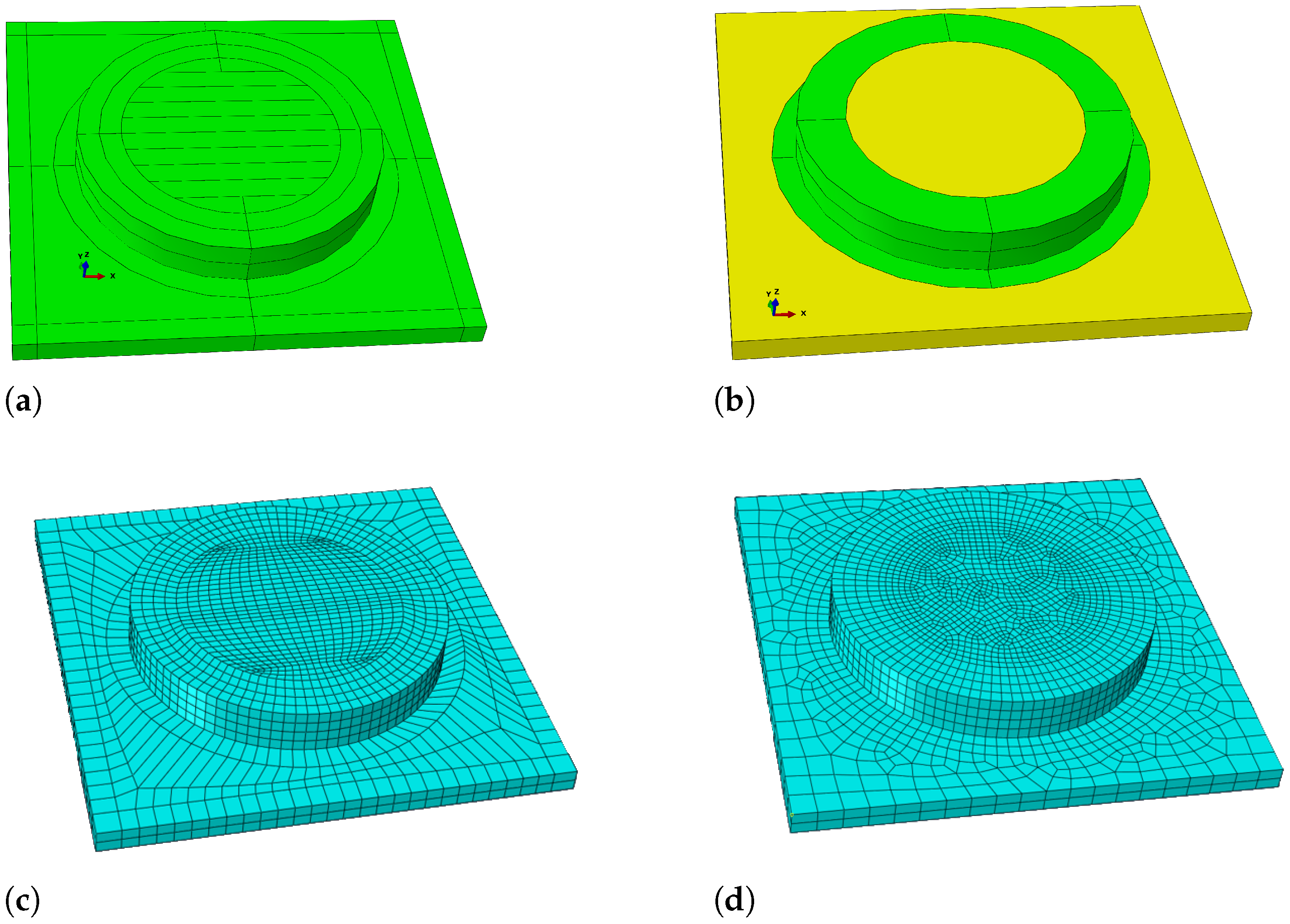
3.3. Variation of Process Parameters

In the WAAM process, process parameters such as welding speed or welding power may need to be varied within a component in order to achieve optimum welding results in all regions. Whether this integrated variation can be mapped by the AM Modeler is to be tested in a further simulation.

The component shown in Figure 17, which consists of a disk-shaped base (green) with an attached pipe section (orange), is used for this purpose. The parameters listed show that a small weld bead with a higher welding feed rate should be simulated for the pipe. For the base, the aim is to simulate a wider weld bead with high material deposition per time. The two regions must be available in the model as individual components in order to be subjected to the path planning individually. This is necessary because the size of the weld bead is taken into account in the path planning and thus influences the number of weld paths.

The result of the thermal simulation carried out is shown in Figure 18. Shown here as a temperature field is the node temperature NT11 at various times during the simulation. Figure 18a shows the production of the base with a wide weld bead and low welding feed. Figure 18b shows the production of the smaller weld bead in the area of the pipe with a higher welding feed rate. All areas shown in gray in the temperature field have a temperature of at least 1400 °C and are therefore in a liquid state.

The lower temperature at the tip of the weld bead is noticeable in both images, which is due to the use of room temperature as the element start temperature. It can also be seen in both temperature fields that the weld beads are not fully heated above 1400 °C, which is due to the estimation of the necessary welding power for the simulation. As the simulation is only intended to test the feasibility of the integrated parameter variation, the welding power is not calculated, but only estimated on the basis of the literature values.

With the functions of the AM Modeler in combination with the developed path planning procedure, parameter variations can be easily implemented in ABAQUS. However, the complexity increases if more than just two areas are equipped with different parameters. The 2020 version of the AM Modeler does not offer any dedicated functions for this purpose and the procedure described does not allow parameters to be varied continuously.

4. Discussion and Conclusions

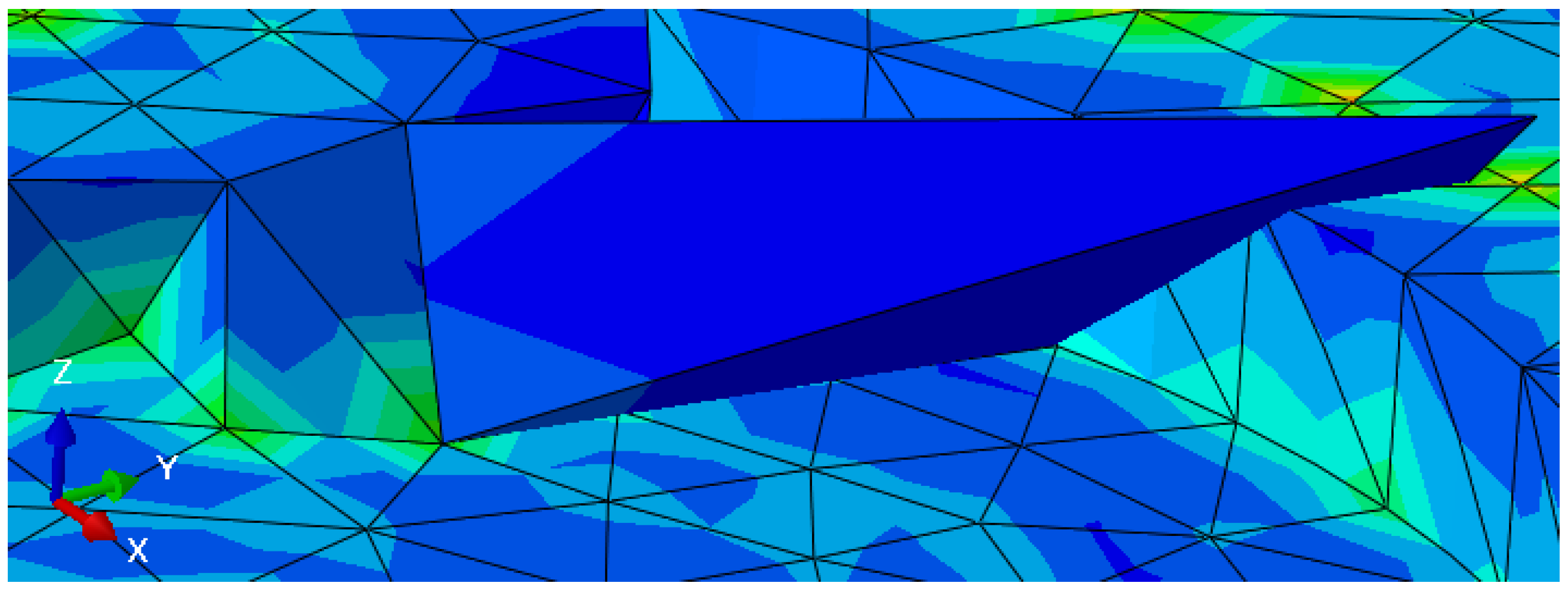
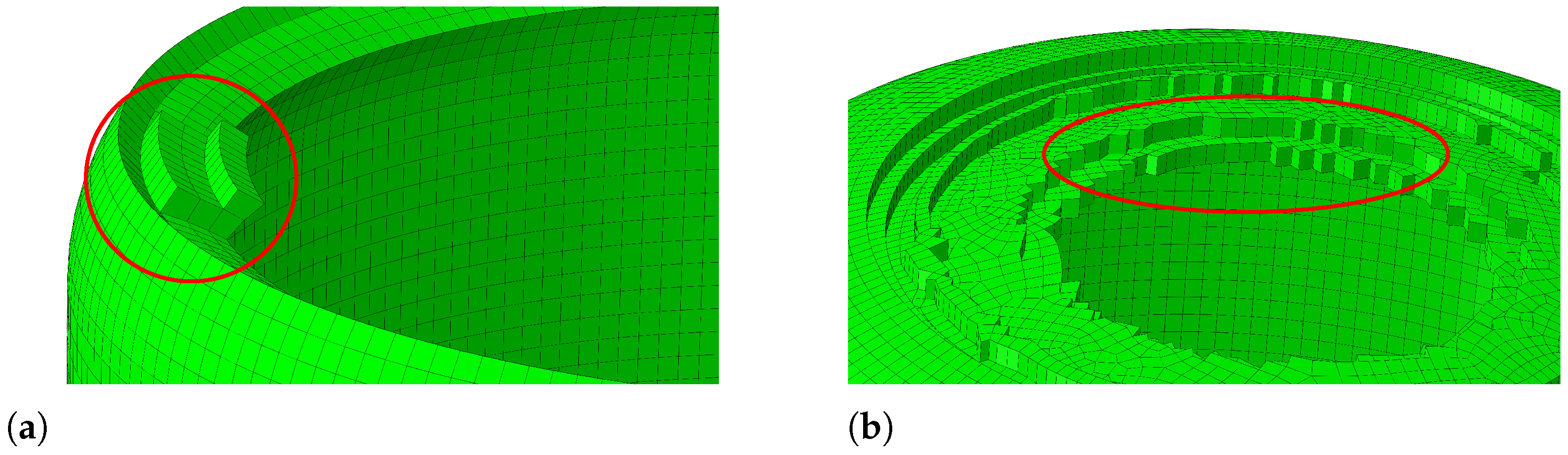
• The investigations into component discretization have revealed various problems that limit the realistic simulation of WAAM with FE modeling. The discretization of components for WAAM can generally be highlighted as a problem in ABAQUS. Depending on the component geometry, the meshing tools provided by ABAQUS are only to a certain extend usable for meshing WAAM components.
• It was also shown that not all element types are suitable for meshing complex, large-scale WAAM components. Here, dedicated meshing programs offer a potential strategy to enable higher quality and more time-efficient meshing in the future.
• Limits in the maximum element size recognized from the investigations further restrict the simulation of WAAM. However, the investigated component geometries are already in a size range that is larger than most of the geometries investigated in the literature. This suggests that similar problems occurred in the studies examined. Extrapolation of the simulation results of individual weld beads to a package of weld beads is conceivable here, which can then be provided with a coarser mesh. In general, simulations of the process in other orders of magnitude offer further potential for a better understanding of the WAAM process.
• Another disadvantage was found in the restriction of the simulation’s axes of motion, which also limits the component geometries that can be simulated with ABAQUS 2020. Here, too, the literature does not yet offer a solution to the problem, as very simple geometries are usually simulated. If geometries with overhangs are also to be simulated in the future, the updated ABAQUS versions must be checked for usability in simulating WAAM. This marks one of the important further developments of the model that would make it possible to model realistic behavior.
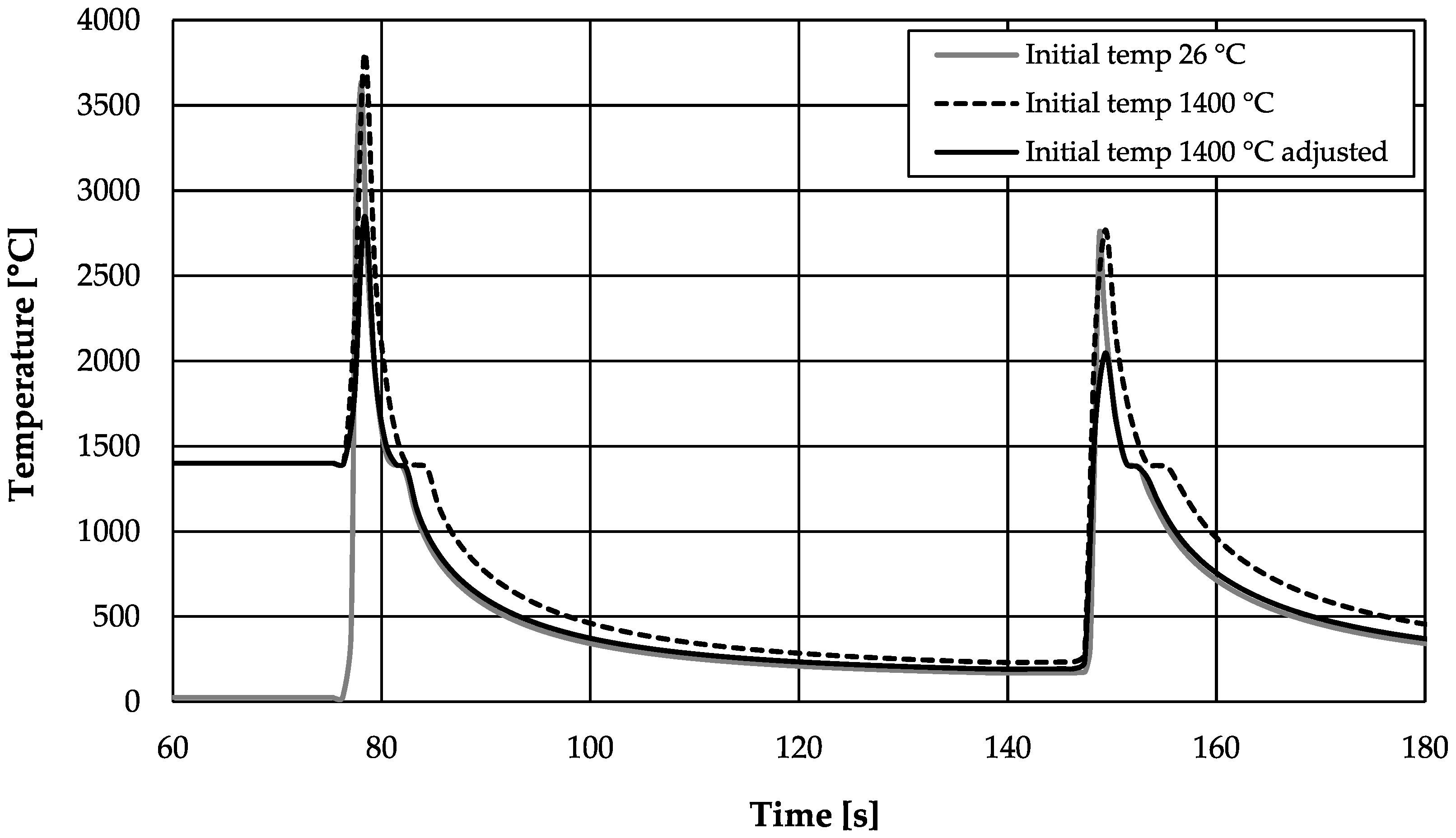
• A use of a high element start temperature in combination with an adapted welding power has proven to be advantageous for process modeling and the stability of the simulation. It is necessary to check whether temperatures even higher than the melting temperature represent the process even better.
• With the AM Modeler, an integrated parameter variation for different areas, which can also occur in the WAAM process, could be realized very easily. Although this is not possible with the AM Modeler by continuously changing the parameters, it still helps to map the WAAM process more realistically.
• An important further step in the development of the simulation model for WAAM is to validate the results using real test components. Here, the component temperature over time can be recorded using thermocouples or thermography and compared with the results of the simulation. Metallography and residual stress measurements also offer the possibility of comparing the real values of mechanical parameters with the simulation results.

References

1. Statistisches Bundesamt, Beschäftigte und Umsatz der Betriebe im Verarbeitenden Gewerbe: Deutschland, Jahre, Wirtschaftszweige. Available online: https://www-genesis.destatis.de/datenbank/online/url/9dbed29c (accessed on 15 March 2025).
2. Kusch, M.; Matthes, K.-J.; Schneider, W. Schweißtechnik: Schweißen von Metallischen Konstruktionswerkstoffen, 7., überarbeitete und Erweiterte Auflage; Hanser: München, Germany, 2022; ISBN 9783446467453. [Google Scholar]
3. Mandeville, M.K.; Brongers, M.P.H.; Tang, F. Quality Assurance and Technology Qualification for Additive Manufacturing of Metallic Pressure Components. In Proceedings of the ASME Pressure Vessels and Piping Conference, Waikoloa, HI, USA, 16–20 July 2017; Zhu, X.-K., Brongers, M., Qian, H., Eds.; The American Society of Mechanical Engineers: New York, NY, USA, 2017. ISBN 978-0-7918-5799-1. [Google Scholar]
4. Bayat, M.; Dong, W.; Thorborg, J.; To, A.C.; Hattel, J.H. A review of multi-scale and multi-physics simulations of metal additive manufacturing processes with focus on modeling strategies. Addit. Manuf. 2021, 47, 102278. [Google Scholar] [CrossRef]
5. Huang, S.; Zhang, T.; Wang, Z.; Cheng, L.; Zha, X.; Guo, B.; Zheng, D.; Xie, H.; Xiang, Z.; Chen, Y.; et al. Asymmetrical cutting-edge design of broaching tool based on FEM simulation. J. Mater. Res. Technol. 2023, 25, 68–82. [Google Scholar] [CrossRef]
6. Almonti, D.; Baiocco, G.; Salvi, D.; Ucciardello, N. Innovative approach for enhancing thermal diffusivity in metal matrix composites using graphene electrodeposition and multi-coating. Int. J. Adv. Manuf. Technol. 2024, 135, 1633–1646. [Google Scholar] [CrossRef]
7. Francois, M.M.; Sun, A.; King, W.E.; Henson, N.J.; Tourret, D.; Bronkhorst, C.A.; Carlson, N.N.; Newman, C.K.; Haut, T.; Bakosi, J.; et al. Modeling of additive manufacturing processes for metals: Challenges and opportunities. Curr. Opin. Solid State Mater. 2017, 21, 198–206. [Google Scholar] [CrossRef]
8. Bargel, H.-J.; Schulze, G. Werkstoffkunde; Eds., 12., bearb. Aufl. 2018; Springer: Berlin/Heidelberg, Germany, 2018; ISBN 9783662486283. [Google Scholar]
9. Karma, A.; Tourret, D. Atomistic to continuum modeling of solidification microstructures. Curr. Opin. Solid State Mater. Sci. 2016, 20, 25–36. [Google Scholar] [CrossRef]
10. Hoyt, J. Atomistic and continuum modeling of dendritic solidification. Mater. Sci. Eng. Rep. 2003, 41, 121–163. [Google Scholar] [CrossRef]
11. Rodgers, T.M.; Madison, J.D.; Tikare, V.; Maguire, M.C. Predicting Mesoscale Microstructural Evolution in Electron Beam Welding. JOM 2016, 68, 1419–1426. [Google Scholar] [CrossRef]
12. Lim, H.; Abdeljawad, F.; Owen, S.J.; Hanks, B.W.; Foulk, J.W.; Battaile, C.C. Incorporating physically-based microstructures in materials modeling: Bridging phase field and crystal plasticity frameworks. Model. Simul. Mater. Sci. Eng. 2016, 24, 45016. [Google Scholar] [CrossRef]
13. Bandyopadhyay, A.; Traxel, K.D. Invited Review Article: Metal-additive manufacturing-Modeling strategies for application-optimized designs. Addit. Manuf. 2018, 22, 758–774. [Google Scholar] [CrossRef]
14. Zhao, H.; Zhang, G.; Yin, Z.; Wu, L. Three-dimensional finite element analysis of thermal stress in single-pass multi-layer weld-based rapid prototyping. J. Mater. Process. Technol. 2012, 212, 276–285. [Google Scholar] [CrossRef]
15. Kaess, M.; Werz, M.; Weihe, S. Residual Stress Formation Mechanisms in Laser Powder Bed Fusion-A Numerical Evaluation. Materials 2023, 16, 2321. [Google Scholar] [CrossRef]
16. Ding, J.; Colegrove, P.; Mehnen, J.; Ganguly, S.; Sequeira Almeida, P.M.; Wang, F.; Williams, S. Thermo-mechanical analysis of Wire and Arc Additive Layer Manufacturing process on large multi-layer parts. Comput. Mater. Sci. 2011, 50, 3315–3322. [Google Scholar] [CrossRef]
17. Fan, Z.; Liou, F. Numerical Modeling of the Additive Manufacturing (AM) Processes of Titanium Alloy. In Titanium Alloys-Towards Achieving Enhanced Properties for Diversified Applications; InTech: Rijeka, Croatia, 2012. [Google Scholar]
18. Mughal, M.P.; Fawad, H.; Mufti, R. Finite element prediction of thermal stresses and deformations in layered manufacturing of metallic parts. Acta Mech. 2006, 183, 61–79. [Google Scholar] [CrossRef]
19. Montevecchi, F.; Venturini, G.; Scippa, A.; Campatelli, G. Finite Element Modelling of Wire-arc-additive-manufacturing Process. Procedia CIRP 2016, 55, 109–114. [Google Scholar] [CrossRef]
20. Chergui, A.; Villeneuve, F.; Béraud, N.; Vignat, F. Thermal simulation of wire arc additive manufacturing: A new material deposition and heat input modelling. Int. J. Interact. Des. Manuf. 2022, 16, 227–237. [Google Scholar] [CrossRef]
21. Ge, J.; Ma, T.; Han, W.; Yuan, T.; Jin, T.; Fu, H.; Xiao, R.; Lei, Y.; Lin, J. Thermal-induced microstructural evolution and defect distribution of wire-arc additive manufacturing 2Cr13 part: Numerical simulation and experimental characterization. Appl. Therm. Eng. 2019, 163, 114335. [Google Scholar] [CrossRef]
22. Graf, M.; Pradjadhiana, K.P.; Hälsig, A.; Manurung, Y.H.P.; Awiszus, B. Numerical simulation of metallic wire arc additive manufacturing (WAAM). Aip Conf. Proc. 2018, 1960, 140010. [Google Scholar]
23. Graf, M.; Hälsig, A.; Höfer, K.; Awiszus, B.; Mayr, P. Thermo-Mechanical Modelling of Wire-Arc Additive Manufacturing (WAAM) of Semi-Finished Products. Metals 2018, 8, 1009. [Google Scholar] [CrossRef]
24. Mughal, M.P.; Mufti, R.A.; Fawad, H. The mechanical effects of deposition patterns in welding-based layered manufacturing. Proc. Inst. Mech. Eng. Part J. Eng. Manuf. 2007, 221, 1499–1509. [Google Scholar] [CrossRef]
25. Zhao, X.F.; Wimmer, A.; Zaeh, M.F. Experimental and simulative investigation of welding sequences on thermally induced distortions in wire arc additive manufacturing. RPJ 2023, 29, 53–63. [Google Scholar] [CrossRef]
26. Amal, M.S.; Justus Panicker, C.T.; Senthilkumar, V. Simulation of wire arc additive manufacturing to find out the optimal path planning strategy. Mater. Today Proc. 2022, 66, 2405–2410. [Google Scholar] [CrossRef]
27. Chiumenti, M.; Cervera, M.; Salmi, A.; Agelet de Saracibar, C.; Dialami, N.; Matsui, K. Finite element modeling of multi-pass welding and shaped metal deposition processes. Comput. Methods Appl. Mech. Eng. 2010, 199, 2343–2359. [Google Scholar] [CrossRef]
28. Israr, R.; Buhl, J.; Elze, L.; Bambach, M. Simulation of different path strategies for wire-arc additive manufacturing with Lagrangian finite element methods. In Proceedings of the LS-Dyna Forum 2018, Bamberg, Germany, 15 October 2018. [Google Scholar]
29. Zhao, Y.; Jia, Y.; Chen, S.; Shi, J.; Li, F. Process planning strategy for wire-arc additive manufacturing: Thermal behavior considerations. Addit. Manuf. 2020, 32, 100935. [Google Scholar] [CrossRef]
30. Xiong, J.; Lei, Y.; Li, R. Finite element analysis and experimental validation of thermal behavior for thin-walled parts in GMAW-based additive manufacturing with various substrate preheating temperatures. Appl. Therm. Eng. 2017, 126, 43–52. [Google Scholar] [CrossRef]
31. Huang, H.; Ma, N.; Chen, J.; Feng, Z.; Murakawa, H. Toward large-scale simulation of residual stress and distortion in wire and arc additive manufacturing. Addit. Manuf. 2020, 34, 101248. [Google Scholar] [CrossRef]
32. Goldak, J.; Chakravarti, A.; Bibby, M. A new finite element model for welding heat sources. Metall. Trans. B 1984, 15, 299–305. [Google Scholar] [CrossRef]
33. Baehr, H.D.; Stephan, K. Wärme- und Stoffübertragung, 10. Auflage; Springer: Berlin/Heidelberg, Germany, 2019; ISBN 978-3-662-58440-8. [Google Scholar]
34. Kuchling, H.; Kuchling, T. Taschenbuch der Physik, 22., Aktualisierte Auflage; Hanser: München, Germany, 2022; ISBN 9783446472747. [Google Scholar]
35. Schuler, V.; Twrdek, J. Praxiswissen Schweißtechnik: Werkstoffe, Prozesse, Fertigung, 6., Vollständig überarbeitete Auflage; Springer: Wiesbaden, Germany; Heidelberg, Germany, 2019. [Google Scholar]
36. 3DA, Materialdatenblatt Edelstahl 316L. Available online: https://www.3d-activation.de/wp-content/uploads/2018/05/1.4404-316L-D.pdf (accessed on 26 March 2025).
Figure 2. Boundary conditions used in all simulations: (a) mechanical boundary conditions; (b) thermal boundary conditions.
Jmmp 09 00166 g002
Figure 3. Temperature-dependent material properties: (a) Flow curve. (b) Young’s modulus. (c) Thermal expansion [15].
Jmmp 09 00166 g003
Figure 4. Simulation geometry for mesh type investigation: (a) Top view. (b) Side view. (c) Hexagonal mesh. (d) Tetragonal mesh.
Jmmp 09 00166 g004
Figure 5. Results for the structural model with tetragonal elements.
Jmmp 09 00166 g005
Figure 6. Heavily deformed element due to high degree of freedom at single nodes.
Jmmp 09 00166 g006
Figure 7. Comparison of element size feasibility: (a) Element size matched with bead size. (b) Element size smaller than bead size. (c) Element size bigger than bead size.
Jmmp 09 00166 g007
Figure 8. (a) Partitioned 3D part. (b) Meshed part (hexagonal elements).
Jmmp 09 00166 g008
Figure 9. Comparison of different meshing techniques: (a) Structured meshing. (b) Structured and Sweep meshing. (c) Structured resulting mesh. (d) Structured and Sweep resulting mesh.
Jmmp 09 00166 g009
Figure 10. Incorrect element activation due to mismatch between mesh and element activation technique.
Jmmp 09 00166 g010
Figure 11. Possible moving axis: (a) Simulation in ABAQUS. (b) Robotic Wire Arc Additive Manufacturing (WAAM).
Jmmp 09 00166 g011
Figure 12. Differences in building direction: (a) Simulation in ABAQUS. (b) Robotic WAAM.
Jmmp 09 00166 g012
Figure 13. Pressure vessel geometry for investigations on element activation.
Jmmp 09 00166 g013
Figure 14. Anomalies in element activation: (a) Tilted elements in wall radius. (b) Activated elements without support in top layers.
Jmmp 09 00166 g014
Figure 15. Deformation of the part due to poor representation of the process.
Jmmp 09 00166 g015
Figure 16. Temperature history in the first two layers for different initial temperatures at same node in the base layer.
Jmmp 09 00166 g016
Figure 17. Variation in process parameters.
Jmmp 09 00166 g017
Figure 18. In-process parameter variation: (a) High weld power and wide bead. (b) Low weld power and narrow bead.
Jmmp 09 00166 g018