
In Situ Active Contour-Based Segmentation and Dimensional Analysis of Part Features in Additive Manufacturing

Abstract
1. Introduction
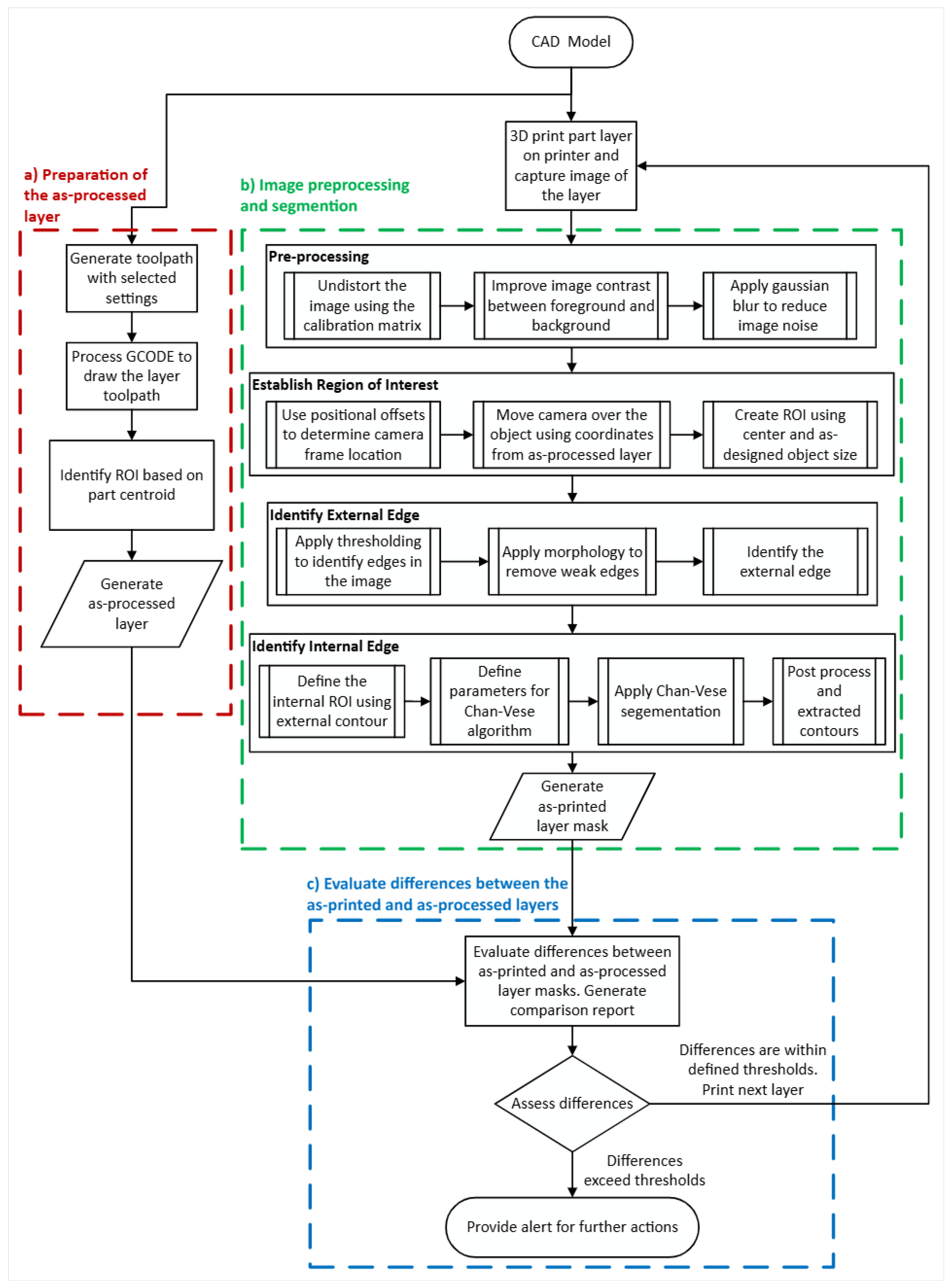
2. Materials and Methods
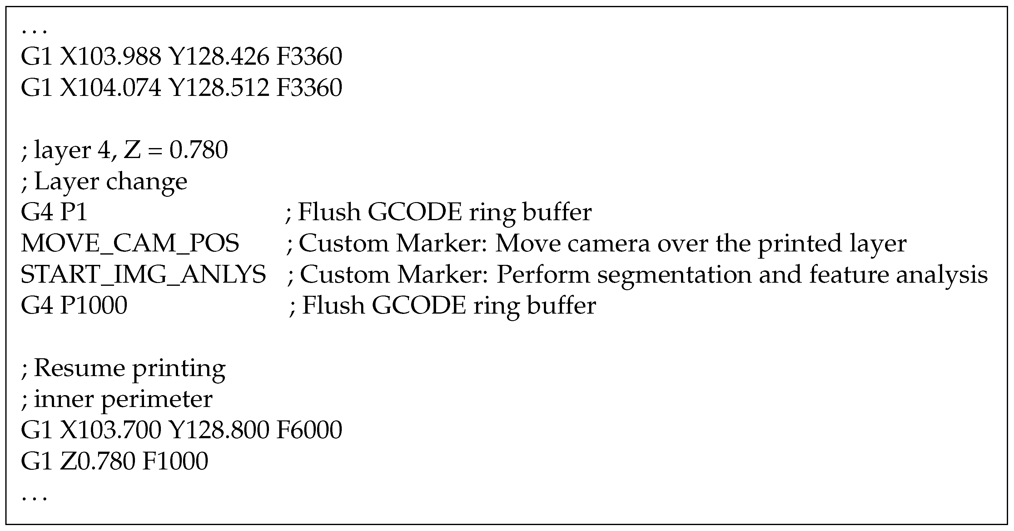
2.1. Prepare the As-Processed Layer
2.2. Acquire and Preprocess a Layer Image
2.3. Image Segmentation
2.3.1. Segmentation Using Thresholding Methods
2.3.2. Active Contour Based Segmentation Using Chan–Vese
- Initial level set: The initial level set function is a signed distance function that represents the initial contour. The shape and size of the initial level set can significantly affect the convergence of the model and the quality of the final segmentation result. Common choices for the shape of the initial level set include simple geometric shapes such as circles or rectangles, placed at strategic locations in the image, or more complex patterns such as a checkerboard. The initial level set function is initialized with the desired contour and is updated iteratively to minimize the energy function. AM parts often contain complex internal features and structures, and simple geometric shapes may not be suitable for the initial level set. Moreover, due to the limited prior knowledge about feature shapes, utilizing complex patterns such as a checkerboard allows for a more flexible and adaptable initialization.
- Intensity weighting parameters and : The intensity weighting parameters control the influence of the intensity term in the energy functional. A higher value of and gives more weight to the intensity term, resulting in a contour that closely follows the intensity boundaries in the image. Generally, both and are set to a similar value, usually 1, which can be effective when the object of interest and the background have similar variability in terms of intensity. Adjusting these values relative to each other, especially in images with significant noise or texture, allows for finer control over the segmentation. This is important for components manufactured through AM in general, as variations in lighting and material properties can significantly affect the quality of image analysis.
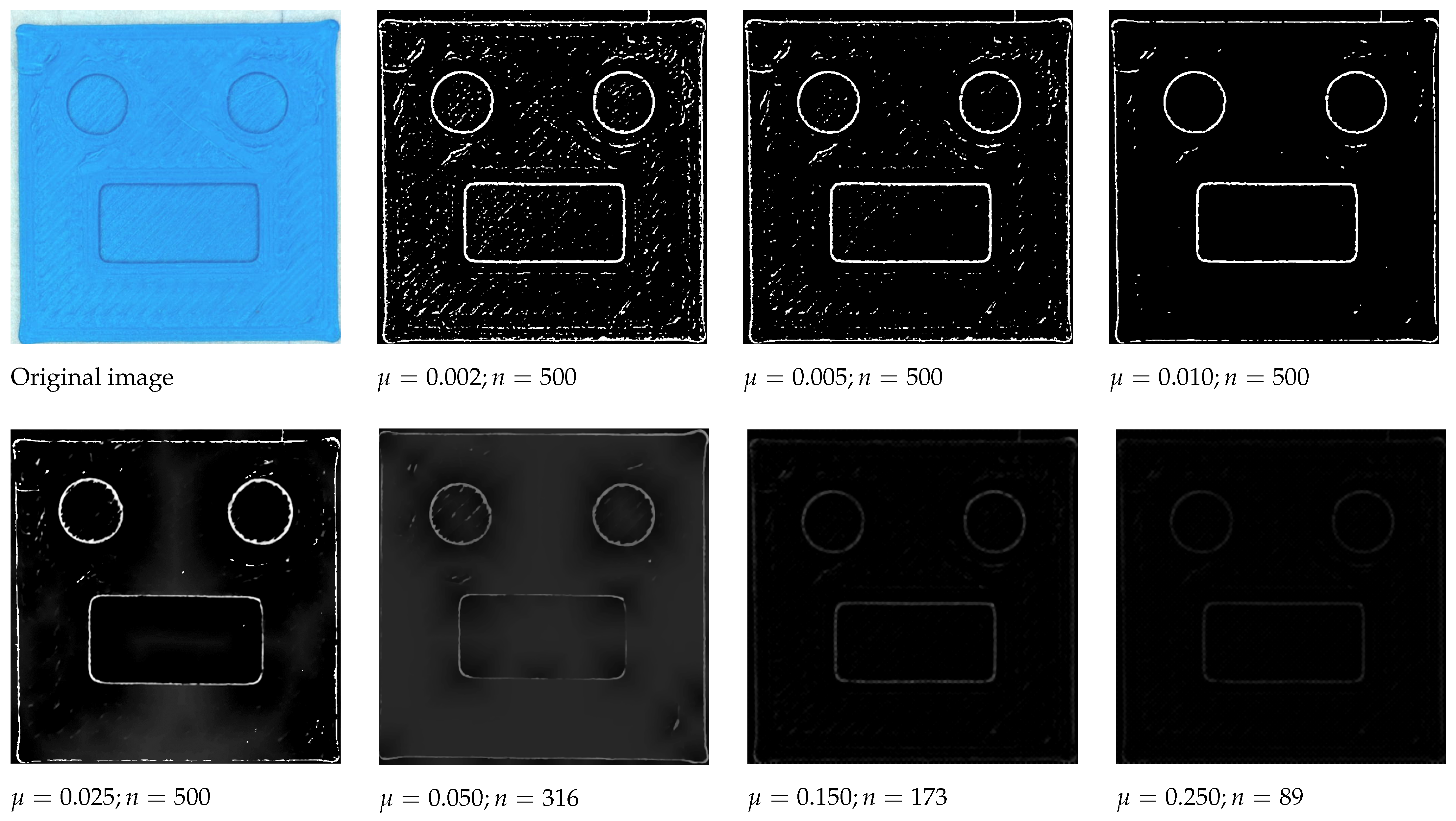
- Contour smoothness parameter : The contour smoothness parameter controls the smoothness of the contour in the segmentation process. Higher values of penalize the length of the contour, resulting in a smoother contour without jagged edges. This is preferable if the acquired image contains a large amount of image noise or texture. However, a very high value might also oversimplify the contour, causing it to miss important features of the object. If images contain fine details, then a lower value of is preferable, as it allows the contour to fit more closely to small features of the object. However, a very low can cause the contour to be too irregular, leading to false edges or inaccuracies in the segmentation. For AM applications, a low value is desirable; however, it is important to preprocess the image to reduce excessive noise. According to the literature, for most applications, a good starting value is [50].
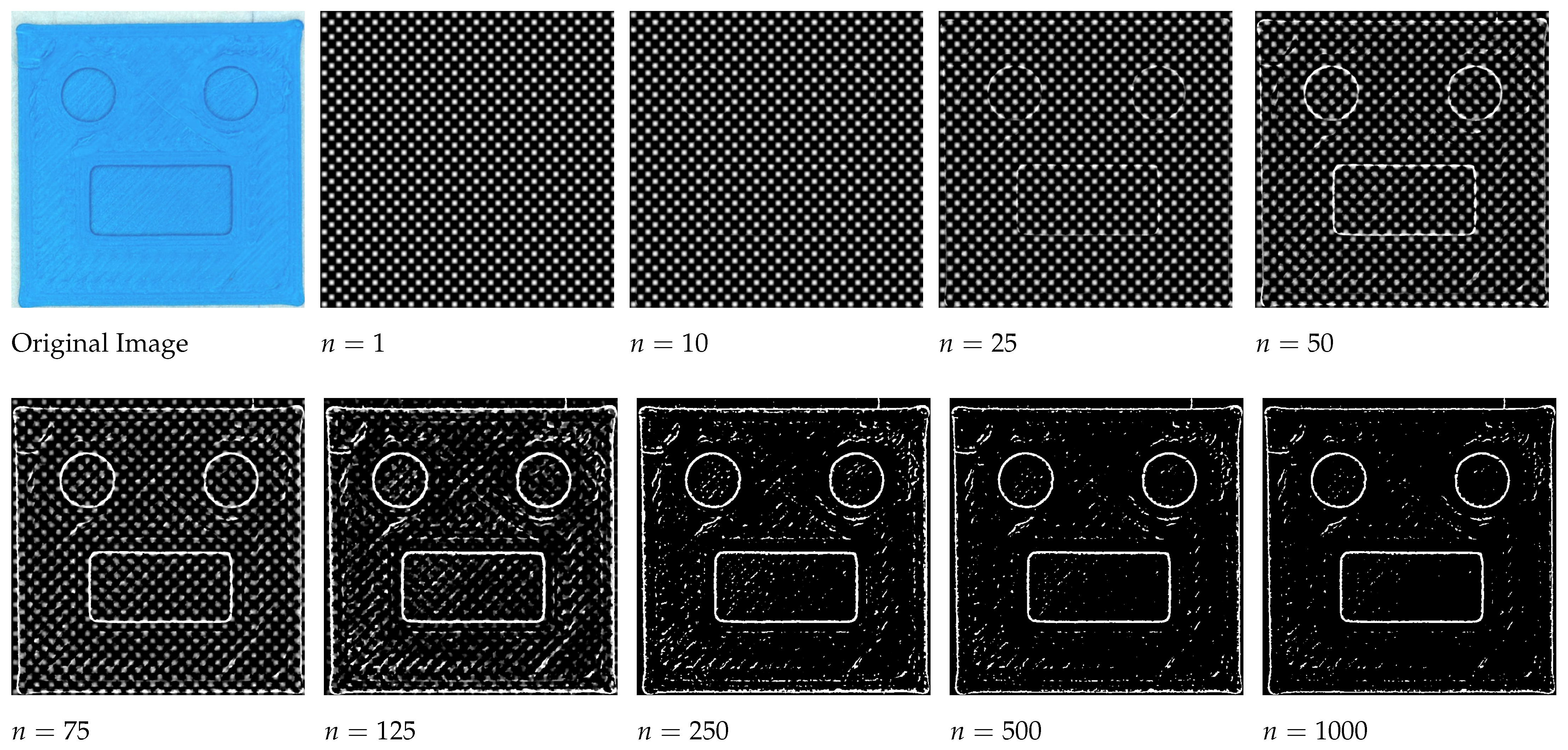
- Iteration limit : The iteration limit specifies the maximum number of iterations the algorithm will execute to minimize the energy function. During each iteration, the algorithm updates the level set function to progressively refine the segmentation until the iteration limit is reached. The choice of the iteration limit is based on the convergence behavior of the algorithm and the desired accuracy of the segmentation results. A higher iteration limit allows the algorithm to refine the segmentation, which can lead to more accurate results. However, it also increases the computation time, an important consideration for AM where the dwell time between layers to process the acquired image affects the overall print time.
2.4. Comparison of the As-Printed with As-Processed Layers
3. Experimental Setup and Configuration
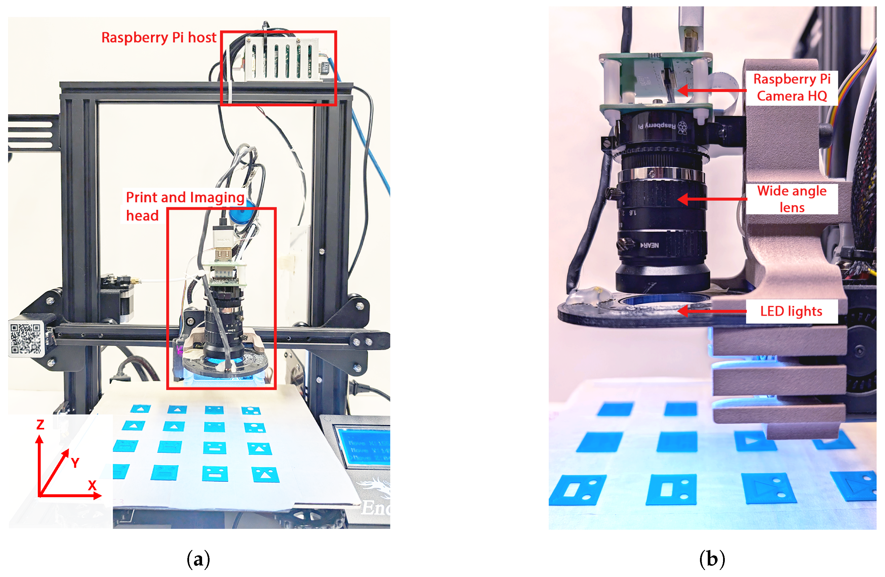
3.1. Additive Manufacturing Platform
3.2. Image Acquisition Setup and Calibration
4. Results
4.1. Effects of Chan–Vese Parameters
4.2. Segmentation Results
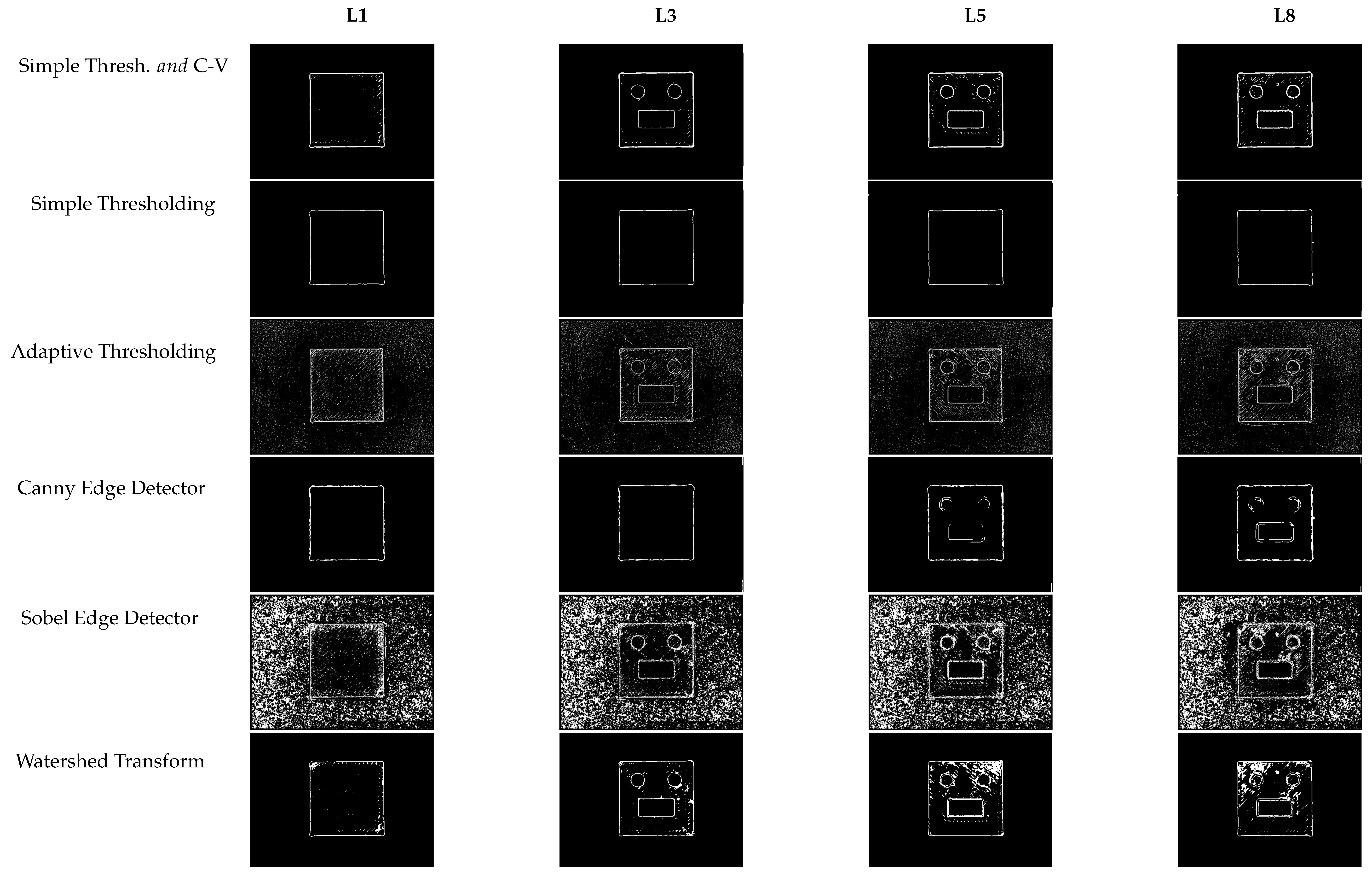
4.2.1. Comparison of Segmentation Methods for the Multilayer Part
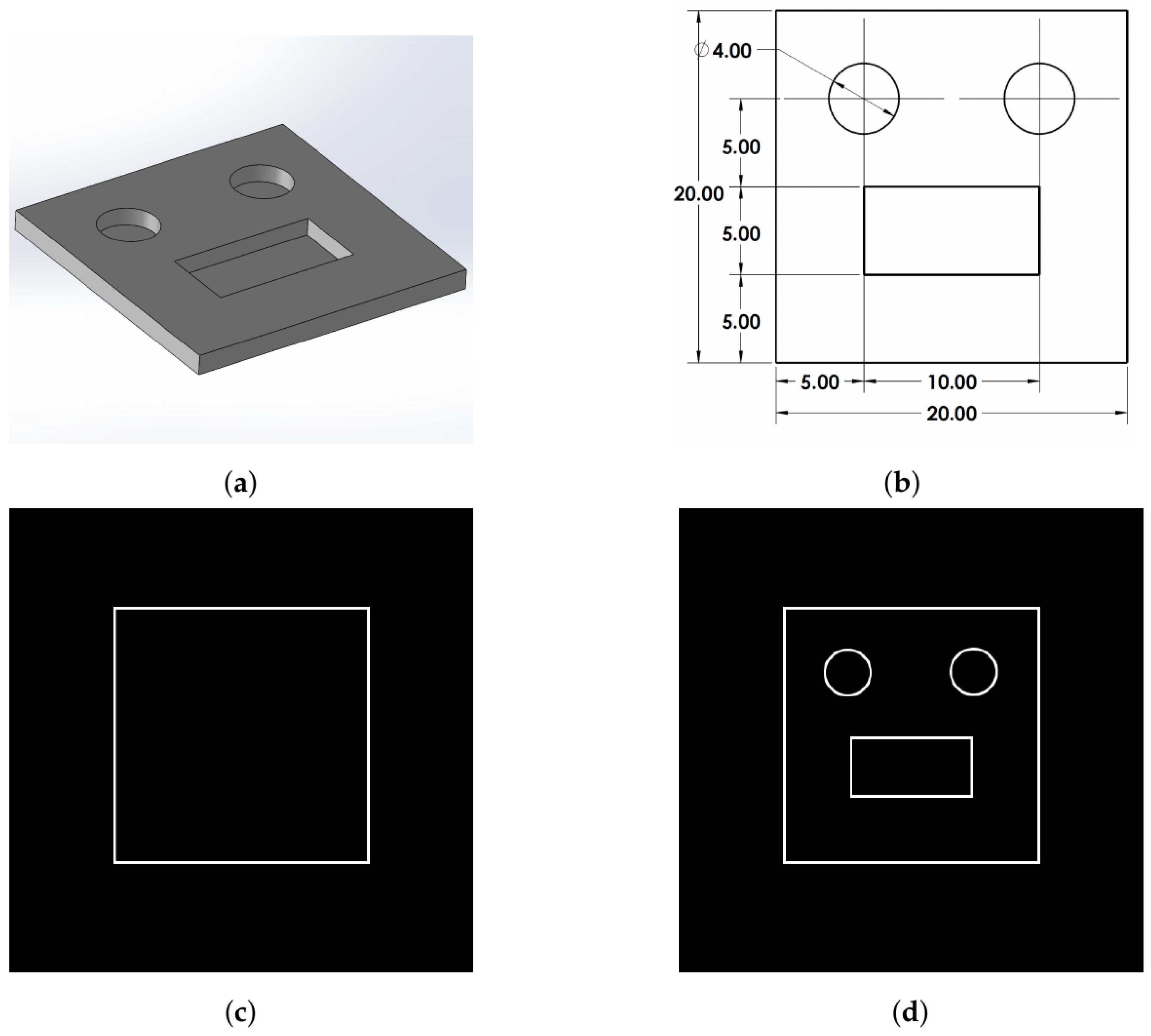
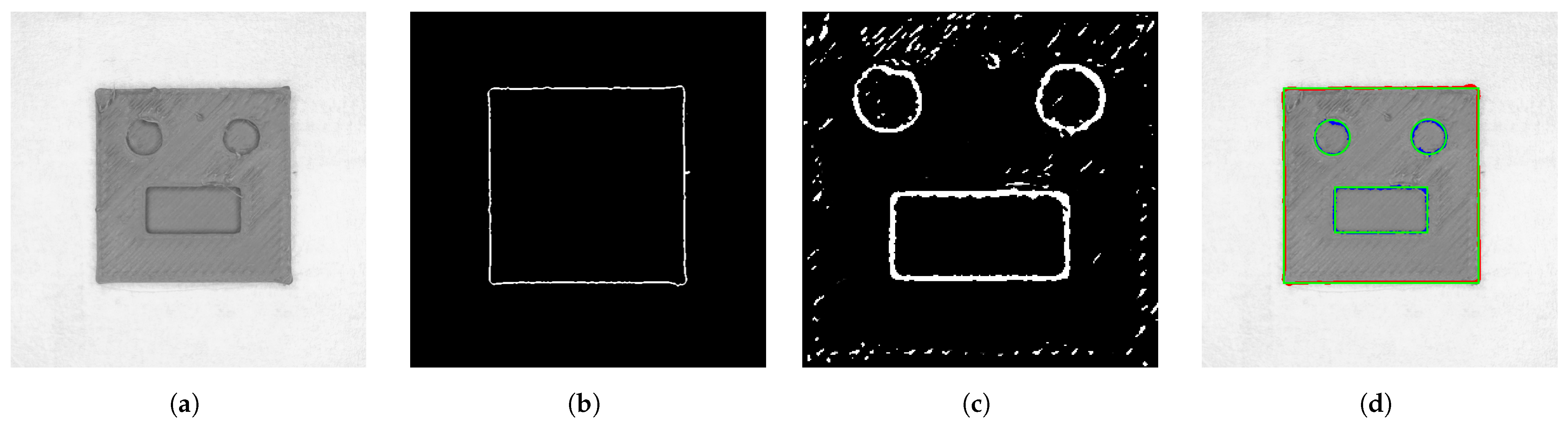
4.2.2. Feature Recognition and Dimensional Analysis
5. Discussion
5.1. Chan–Vese Parameters
5.2. Segmentation of AM Components
5.3. Feature Recognition and Evaluation
6. Conclusions
Author Contributions
Funding
Data Availability Statement
Acknowledgments
Conflicts of Interest
Abbreviations
| AM | Additive Manufacturing |
| C–V | Chan–Vese |
| FDM | Fused Deposition Modeling |
| DT | Digital Twin |
| CNN | Convolutional Neural Network |
| LPBF | Laser Powder Bed Fusion |
| CAD | Computer-Aided Design |
| STL | Standard Tessellation Language |
| GCODE | Geometric Code |
| RoI | Region of Interest |
| FoV | Field of View |
| MPFS | Minimum Printable Feature Size |
References
- Barcena, A.J.R.; Ravi, P.; Kundu, S.; Tappa, K. Emerging Biomedical and Clinical Applications of 3D-Printed Poly(Lactic Acid)-Based Devices and Delivery Systems. Bioengineering 2024, 11, 705. [Google Scholar] [CrossRef] [PubMed]
- Patel, P.; Ravi, P.; Shiakolas, P.; Welch, T.; Saini, T. Additive manufacturing of heterogeneous bio-resorbable constructs for soft tissue applications. In Proceedings of the Materials Science and Technology 2018, MS and T 2018, Columbus, OH, USA, 14–18 October 2018; pp. 1496–1503. [Google Scholar] [CrossRef]
- Adejokun, S.A.; Kumat, S.S.; Shiakolas, P.S. A Microrobot with an Attached Microforce Sensor for Transurethral Access to the Bladder Interior Wall. J. Eng. Sci. Med. Diagn. Ther. 2023, 6, 031001. [Google Scholar] [CrossRef]
- Martelli, A.; Bellucci, D.; Cannillo, V. Additive Manufacturing of Polymer/Bioactive Glass Scaffolds for Regenerative Medicine: A Review. Polymers 2023, 15, 2473. [Google Scholar] [CrossRef]
- Wang, J.; Shao, C.; Wang, Y.; Sun, L.; Zhao, Y. Microfluidics for Medical Additive Manufacturing. Engineering 2020, 6, 1244–1257. [Google Scholar] [CrossRef]
- Hazra, S.; Abdul Rahaman, A.H.; Shiakolas, P.S. An Affordable Telerobotic System Architecture for Grasp Training and Object Grasping for Human–Machine Interaction. J. Eng. Sci. Med. Diagn. Ther. 2024, 7, 011011. [Google Scholar] [CrossRef]
- Salifu, S.; Desai, D.; Ogunbiyi, O.; Mwale, K. Recent development in the additive manufacturing of polymer-based composites for automotive structures—A review. Int. J. Adv. Manuf. Technol. 2022, 119, 6877–6891. [Google Scholar] [CrossRef]
- Saini, T.; Shiakolas, P.; Dhal, K. In-Situ Fabrication of Electro-Mechanical Structures Using Multi-Material and Multi-Process Additive Manufacturing. In Proceedings of the Contributed Papers from MS&T17, MS&T18, Columbus, OH, USA, 14–18 October 2018; pp. 49–55. [Google Scholar] [CrossRef]
- Ravi, P.; Shiakolas, P.S.; Welch, T.; Saini, T.; Guleserian, K.; Batra, A.K. On the Capabilities of a Multi-Modality 3D Bioprinter for Customized Biomedical Devices. In Proceedings of the ASME International Mechanical Engineering Congress and Exposition, Houston, TX, USA, 13–19 November 2015; Volume 2A, p. V02AT02A008. [Google Scholar] [CrossRef]
- Shen, C.; Hua, X.; Li, F.; Zhang, T.; Li, Y.; Zhang, Y.; Wang, L.; Ding, Y.; Zhang, P.; Lu, Q. Composition-induced microcrack defect formation in the twin-wire plasma arc additive manufacturing of binary TiAl alloy: An X-ray computed tomography-based investigation. J. Mater. Res. 2021, 36, 4974–4985. [Google Scholar] [CrossRef]
- Ziabari, A.; Venkatakrishnan, S.V.; Snow, Z.; Lisovich, A.; Sprayberry, M.; Brackman, P.; Frederick, C.; Bhattad, P.; Graham, S.; Bingham, P.; et al. Enabling rapid X-ray CT characterisation for additive manufacturing using CAD models and deep learning-based reconstruction. NPJ Comput. Mater. 2023, 9, 91. [Google Scholar] [CrossRef]
- Rieder, H.; Dillhöfer, A.; Spies, M.; Bamberg, J.; Hess, T. Online Monitoring of Additive Manufacturing Processes Using Ultrasound. Available online: https://api.semanticscholar.org/CorpusID:26787041 (accessed on 8 June 2024).
- Mireles, J.; Ridwan, S.; Morton, P.A.; Hinojos, A.; Wicker, R.B. Analysis and correction of defects within parts fabricated using powder bed fusion technology. Surf. Topogr. Metrol. Prop. 2015, 3, 034002. [Google Scholar] [CrossRef]
- Du Plessis, A.; Le Roux, S.G.; Els, J.; Booysen, G.; Blaine, D.C. Application of microCT to the non-destructive testing of an additive manufactured titanium component. Case Stud. Nondestruct. Test. Eval. 2015, 4, 1–7. [Google Scholar] [CrossRef]
- Du Plessis, A.; Le Roux, S.G.; Booysen, G.; Els, J. Quality Control of a Laser Additive Manufactured Medical Implant by X-ray Tomography. 3D Print. Addit. Manuf. 2016, 3, 175–182. [Google Scholar] [CrossRef]
- Cerniglia, D.; Scafidi, M.; Pantano, A.; Łopatka, R. Laser Ultrasonic Technique for Laser Powder Deposition Inspection. Available online: https://www.ndt.net/?id=15510 (accessed on 25 August 2024).
- Lu, L.; Hou, J.; Yuan, S.; Yao, X.; Li, Y.; Zhu, J. Deep learning-assisted real-time defect detection and closed-loop adjustment for additive manufacturing of continuous fiber-reinforced polymer composites. Robot. Comput.-Integr. Manuf. 2023, 79, 102431. [Google Scholar] [CrossRef]
- Garanger, K.; Khamvilai, T.; Feron, E. 3D Printing of a Leaf Spring: A Demonstration of Closed-Loop Control in Additive Manufacturing. In Proceedings of the 2018 IEEE Conference on Control Technology and Applications (CCTA), Copenhagen, Denmark, 21–24 August 2018; pp. 465–470. [Google Scholar] [CrossRef]
- Cummings, I.T.; Bax, M.E.; Fuller, I.J.; Wachtor, A.J.; Bernardin, J.D. A Framework for Additive Manufacturing Process Monitoring & Control. In Topics in Modal Analysis & Testing, Volume 10; Mains, M., Blough, J., Eds.; Conference Proceedings of the Society for Experimental Mechanics Series; Springer International Publishing: Cham, Switzerland, 2017; pp. 137–146. [Google Scholar] [CrossRef]
- He, K.; Zhang, Q.; Hong, Y. Profile monitoring based quality control method for fused deposition modeling process. J. Intell. Manuf. 2019, 30, 947–958. [Google Scholar] [CrossRef]
- Baumann, F.; Roller, D. Vision based error detection for 3D printing processes. MATEC Web Conf. 2016, 59, 06003. [Google Scholar] [CrossRef]
- Lyngby, R.; Wilm, J.; Eiríksson, E.; Nielsen, J.; Jensen, J.; Aanæs, H.; Pedersen, D. In-line 3D print failure detection using computer vision. In Proceedings of the Dimensional Accuracy and Surface Finish in Additive Manufacturing, Leuven, Belgium, 10–11 October 2017. [Google Scholar]
- Yi, W.; Ketai, H.; Xiaomin, Z.; Wenying, D. Machine vision based statistical process control in fused deposition modeling. In Proceedings of the 2017 12th IEEE Conference on Industrial Electronics and Applications (ICIEA), Siem Reap, Cambodia, 18–20 June 2017; pp. 936–941. [Google Scholar] [CrossRef]
- Delli, U.; Chang, S. Automated Process Monitoring in 3D Printing Using Supervised Machine Learning; Elsevier: Amsterdam, The Netherlands, 2018; Volume 26, pp. 865–870. ISSN 23519789. [Google Scholar] [CrossRef]
- Shen, H.; Sun, W.; Fu, J. Multi-view online vision detection based on robot fused deposit modeling 3D printing technology. Rapid Prototyp. J. 2019, 25, 343–355. [Google Scholar] [CrossRef]
- Gaikwad, A.; Yavari, R.; Montazeri, M.; Cole, K.; Bian, L.; Rao, P. Toward the digital twin of additive manufacturing: Integrating thermal simulations, sensing, and analytics to detect process faults. IISE Trans. 2020, 52, 1204–1217. [Google Scholar] [CrossRef]
- Knapp, G.L.; Mukherjee, T.; Zuback, J.S.; Wei, H.L.; Palmer, T.A.; De, A.; DebRoy, T. Building blocks for a digital twin of additive manufacturing. Acta Mater. 2017, 135, 390–399. [Google Scholar] [CrossRef]
- Nath, P.; Mahadevan, S. Probabilistic Digital Twin for Additive Manufacturing Process Design and Control. J. Mech. Des. 2022, 144, 091704. [Google Scholar] [CrossRef]
- Farhan Khan, M.; Alam, A.; Ateeb Siddiqui, M.; Saad Alam, M.; Rafat, Y.; Salik, N.; Al-Saidan, I. Real-time defect detection in 3D printing using machine learning. Mater. Today Proc. 2021, 42, 521–528. [Google Scholar] [CrossRef]
- Liu, C.; Law, A.C.C.; Roberson, D.; Kong, Z.J. Image analysis-based closed loop quality control for additive manufacturing with fused filament fabrication. J. Manuf. Syst. 2019, 51, 75–86. [Google Scholar] [CrossRef]
- Ye, Z.; Liu, C.; Tian, W.; Kan, C. In-situ point cloud fusion for layer-wise monitoring of additive manufacturing. J. Manuf. Syst. 2021, 61, 210–222. [Google Scholar] [CrossRef]
- Rossi, A.; Moretti, M.; Senin, N. Layer inspection via digital imaging and machine learning for in-process monitoring of fused filament fabrication. J. Manuf. Process. 2021, 70, 438–451. [Google Scholar] [CrossRef]
- Moretti, M.; Rossi, A.; Senin, N. In-process monitoring of part geometry in fused filament fabrication using computer vision and digital twins. Addit. Manuf. 2021, 37, 101609. [Google Scholar] [CrossRef]
- Castro, P.; Pathinettampadian, G.; Thanigainathan, S.; Prabakar, V.; Krishnan, R.A.; Subramaniyan, M.K. Measurement of additively manufactured part dimensions using OpenCV for process monitoring. J. Process. Mech. Eng. 2024, 09544089241227894. [Google Scholar] [CrossRef]
- Nuchitprasitchai, S.; Roggemann, M.; Pearce, J. Three Hundred and Sixty Degree Real-Time Monitoring of 3-D Printing Using Computer Analysis of Two Camera Views. JMMP 2017, 1, 2. [Google Scholar] [CrossRef]
- Holzmond, O.; Li, X. In situ real time defect detection of 3D printed parts. Addit. Manuf. 2017, 17, 135–142. [Google Scholar] [CrossRef]
- Lyu, J.; Manoochehri, S. Online Convolutional Neural Network-based anomaly detection and quality control for Fused Filament Fabrication process. Virtual Phys. Prototyp. 2021, 16, 160–177. [Google Scholar] [CrossRef]
- Saini, T.; Shiakolas, P.S. A Framework for In-Situ Vision Based Detection of Part Features and its Single Layer Verification for Additive Manufacturing. In Proceedings of the ASME International Mechanical Engineering Congress and Exposition, New Orleans, LA, USA, 29 October–2 November 2023; Volume 3, p. V003T03A083. [Google Scholar] [CrossRef]
- Saini, T.; Shiakolas, P.S.; McMurrough, C. Evaluation of Image Segmentation Methods for In Situ Quality Assessment in Additive Manufacturing. Metrology 2024, 4, 598–618. [Google Scholar] [CrossRef]
- Gunasekara, S.R.; Kaldera, H.N.T.K.; Dissanayake, M.B. A Systematic Approach for MRI Brain Tumor Localization and Segmentation Using Deep Learning and Active Contouring. J. Healthc. Eng. 2021, 2021, 6695108. [Google Scholar] [CrossRef]
- Fang, J.; Wang, K. Weld Pool Image Segmentation of Hump Formation Based on Fuzzy C-Means and Chan-Vese Model. J. Mater. Eng. Perform. 2019, 28, 4467–4476. [Google Scholar] [CrossRef]
- Caltanissetta, F.; Grasso, M.; Petrò, S.; Colosimo, B.M. Characterization of in situ measurements based on layerwise imaging in laser powder bed fusion. Addit. Manuf. 2018, 24, 183–199. [Google Scholar] [CrossRef]
- Li, Z.; Liu, X.; Wen, S.; He, P.; Zhong, K.; Wei, Q.; Shi, Y.; Liu, S. In Situ 3D Monitoring of Geometric Signatures in the Powder-Bed-Fusion Additive Manufacturing Process via Vision Sensing Methods. Sensors 2018, 18, 1180. [Google Scholar] [CrossRef]
- Python Software Foundation. What is New In Python 3.10. Available online: https://docs.python.org/3/whatsnew/3.10.html (accessed on 2 February 2024).
- Kass, M.; Witkin, A.; Terzopoulos, D. Snakes: Active contour models. Int. J. Comput. Vis. 1988, 1, 321–331. [Google Scholar] [CrossRef]
- Mumford, D.; Shah, J. Optimal approximations by piecewise smooth functions and associated variational problems. Commun. Pure Appl. Math. 1989, 42, 577–685. [Google Scholar] [CrossRef]
- Chan, T.; Vese, L. An Active Contour Model without Edges. In Scale-Space Theories in Computer Vision; Lecture Notes in Computer Science; Springer: Berlin/Heidelberg, Germany, 1999; Volume 1682, pp. 141–151. [Google Scholar] [CrossRef]
- Osher, S.; Sethian, J.A. Fronts propagating with curvature-dependent speed: Algorithms based on Hamilton-Jacobi formulations. J. Comput. Physics 1988, 79, 12–49. [Google Scholar] [CrossRef]
- Cohen, R. The Chan-Vese Algorithm. Technical report, Israel Institute of Technology. arXiv 2011, arXiv:1107.2782. [Google Scholar] [CrossRef]
- Getreuer, P. Chan-Vese Segmentation. Image Process. Line 2012, 2, 214–224. [Google Scholar] [CrossRef]
- Wang, X.F.; Huang, D.S.; Xu, H. An efficient local Chan–Vese model for image segmentation. Pattern Recognit. 2010, 43, 603–618. [Google Scholar] [CrossRef]
- Ramer, U. An iterative procedure for the polygonal approximation of plane curves. Comput. Graph. Image Process. 1972, 1, 244–256. [Google Scholar] [CrossRef]
- Douglas, D.H.; Peucker, T.K. Algorithms for the Reduction of the Number of Points Required to Represent a Digitized Line or its Caricature. Cartogr. Int. J. Geogr. Inf. Geovisualization 1973, 10, 112–122. [Google Scholar] [CrossRef]
- Ming-Kuei, H. Visual pattern recognition by moment invariants. IEEE Trans. Inf. Theory 1962, 8, 179–187. [Google Scholar] [CrossRef]
- Shenzhen Creality 3D Technology Co., Ltd. Creality Ender 3 Pro. Available online: https://www.creality.com/products/ender-3-pro-3d-printer (accessed on 17 January 2024).
- Raspberry Pi Foundation. Raspberry Pi 2 Model B. Available online: https://www.raspberrypi.com/products/raspberry-pi-2-model-b/ (accessed on 17 January 2024).
- O’Connor, K. Klipper Firmware. Available online: https://www.klipper3d.org/Features.html (accessed on 17 January 2024).
- OpenCV. OpenCV 4.6.0. Available online: https://docs.opencv.org/4.6.0 (accessed on 9 April 2024).
- Raspberry Pi Foundation. Raspberry Pi HQ Camera. Available online: https://www.raspberrypi.com/products/raspberry-pi-high-quality-camera/ (accessed on 17 January 2024).
- Sony Semiconductor Solutions Corporation. Image Sensor for Consumer Cameras. Available online: https://www.sony-semicon.com/en/products/is/camera/index.html (accessed on 18 March 2025).
- Hartley, R.; Zisserman, A. Camera Models. In Multiple View Geometry in Computer Vision, 2nd ed.; Cambridge University Press: Cambridge, UK, 2004; pp. 153–177. ISBN 0521540518. [Google Scholar]
- OpenCV. Camera Calibration with OpenCV. Available online: https://docs.opencv.org/4.x/d4/d94/tutorial_camera_calibration.html (accessed on 9 April 2024).
- Duda, R.O.; Hart, P.E. Use of the Hough transformation to detect lines and curves in pictures. Commun. ACM 1972, 15, 11–15. [Google Scholar] [CrossRef]
- Scikit-Image Team. Chan-Vese Segmentation. Available online: https://scikit-image.org/docs/stable/auto_examples/segmentation/plot_chan_vese.html (accessed on 21 July 2023).

| Parameter | Value |
|---|---|
| Layer Height (mm) | 0.2 |
| Perimeters | 3 |
| Extrusion Width for all features (mm) | 0.4 |
| Fill Density | 100% |
| Fill Pattern | Rectilinear |
| Layer Number | Method | Accuracy (%) | Precision (%) | Recall (%) | Jaccard Index (%) |
|---|---|---|---|---|---|
| L1 | Simple Thresh. Chan–Vese | 99.620 | 81.620 | 94.540 | 78.340 |
| Simple thresholding | 99.340 | 59.810 | 89.850 | 56.020 | |
| Adaptive thresholding | 95.060 | 56.420 | 15.490 | 13.830 | |
| Sobel edge detector | 82.220 | 85.170 | 6.380 | 6.310 | |
| Canny edge detector | 99.410 | 69.320 | 85.900 | 62.240 | |
| Watershed transform | 97.730 | 62.750 | 33.600 | 28.010 | |
| L3 | Simple Thresh. Chan–Vese | 99.120 | 84.320 | 76.510 | 67.190 |
| Simple thresholding | 97.410 | 35.980 | 43.260 | 24.450 | |
| Adaptive thresholding | 94.280 | 45.720 | 19.260 | 15.680 | |
| Sobel edge detector | 79.160 | 73.800 | 7.820 | 7.610 | |
| Canny edge detector | 98.270 | 35.110 | 78.470 | 32.030 | |
| Watershed transform | 97.260 | 63.450 | 43.860 | 35.020 | |
| L5 | Simple Thresh. Chan–Vese | 99.010 | 76.870 | 82.270 | 66.030 |
| Simple thresholding | 97.410 | 35.500 | 43.050 | 24.150 | |
| Adaptive thresholding | 93.010 | 49.740 | 16.590 | 14.210 | |
| Sobel edge detector | 76.660 | 72.740 | 6.940 | 6.760 | |
| Canny edge detector | 97.950 | 42.380 | 58.220 | 32.500 | |
| Watershed transform | 95.560 | 66.460 | 29.690 | 25.820 | |
| L8 | Simple Thresh. Chan–Vese | 98.770 | 70.770 | 80.170 | 60.340 |
| Simple thresholding | 97.380 | 35.150 | 42.440 | 23.800 | |
| Adaptive thresholding | 93.270 | 53.580 | 18.090 | 15.640 | |
| Sobel edge detector | 74.950 | 74.630 | 6.630 | 6.480 | |
| Canny edge detector | 97.790 | 47.260 | 52.760 | 33.190 | |
| Watershed transform | 95.330 | 58.460 | 26.840 | 22.540 |
| Feature | Height | Width | Number of Sides | ||||
|---|---|---|---|---|---|---|---|
| As-Processed | As-Printed | Diff. | As-Processed | As-Printed | Diff. | ||
| External Geometry (pixels) | 800 | 806 | 6 | 800 | 797 | −3 | 4 |
| External Geometry (mm) | 20.000 | 20.150 | 0.150 | 20.000 | 19.925 | −0.075 | |
| Internal Circle-left (pixels) | 160 | 153 | −7 | 160 | 154 | −6 | 19 |
| Internal Circle-left (mm) | 4.000 | 3.825 | −0.175 | 4.000 | 3.850 | −0.150 | |
| Internal Circle-right (pixels) | 160 | 150 | −10 | 160 | 152 | -8 | 14 |
| Internal Circle-right (mm) | 4.000 | 3.750 | −0.250 | 4.000 | 3.800 | −0.200 | |
| Internal Rectangle (pixels) | 200 | 199 | −1 | 400 | 405 | 5 | 4 |
| Internal Rectangle (mm) | 5.000 | 4.975 | −0.025 | 10.000 | 10.125 | 0.125 | |
Disclaimer/Publisher’s Note: The statements, opinions and data contained in all publications are solely those of the individual author(s) and contributor(s) and not of MDPI and/or the editor(s). MDPI and/or the editor(s) disclaim responsibility for any injury to people or property resulting from any ideas, methods, instructions or products referred to in the content. |
© 2025 by the authors. Licensee MDPI, Basel, Switzerland. This article is an open access article distributed under the terms and conditions of the Creative Commons Attribution (CC BY) license (https://creativecommons.org/licenses/by/4.0/).
Share and Cite
Saini, T.; Shiakolas, P.S. In Situ Active Contour-Based Segmentation and Dimensional Analysis of Part Features in Additive Manufacturing. J. Manuf. Mater. Process. 2025, 9, 102. https://doi.org/10.3390/jmmp9030102
Saini T, Shiakolas PS. In Situ Active Contour-Based Segmentation and Dimensional Analysis of Part Features in Additive Manufacturing. Journal of Manufacturing and Materials Processing. 2025; 9(3):102. https://doi.org/10.3390/jmmp9030102
Chicago/Turabian StyleSaini, Tushar, and Panos S. Shiakolas. 2025. "In Situ Active Contour-Based Segmentation and Dimensional Analysis of Part Features in Additive Manufacturing" Journal of Manufacturing and Materials Processing 9, no. 3: 102. https://doi.org/10.3390/jmmp9030102
APA StyleSaini, T., & Shiakolas, P. S. (2025). In Situ Active Contour-Based Segmentation and Dimensional Analysis of Part Features in Additive Manufacturing. Journal of Manufacturing and Materials Processing, 9(3), 102. https://doi.org/10.3390/jmmp9030102