Effect of Intermediate Path on Post-Wrinkle Initiation of the Multi-Pass Metal Spinning Process: Analysis in the Rotating Reference Frame

Abstract

The metal spinning process has been observed in recent major investigations carried out using finite element analysis. One interesting idea has proposed simulating a rotating disc for the simulation of the metal spinning process to reduce computational time. The development of this concept is presented in this paper, including the formal mathematical transformation from the inertial frame to the rotating reference frame, specific FEM configurations with mesh sizes based on a minimized aspect ratio, a mesh convergence study, and the application of a feed rate scale. Furthermore, in the context of the rotating reference frame, the flange geometry after wrinkle initiation is investigated, including the number of peaks and their amplitudes. Using this new approach, it was found that the number of peaks gradually increases from two to eight peaks while their amplitude decreases. In the case of severe wrinkles, the number of peaks stays at four while the amplitude increases dramatically. The intermediate path proves capable of increasing the number of peaks while maintaining a low amplitude. These results will make it possible to design new paths, facilitating the production of defect-free spun parts.

1. Introduction and Literature Review

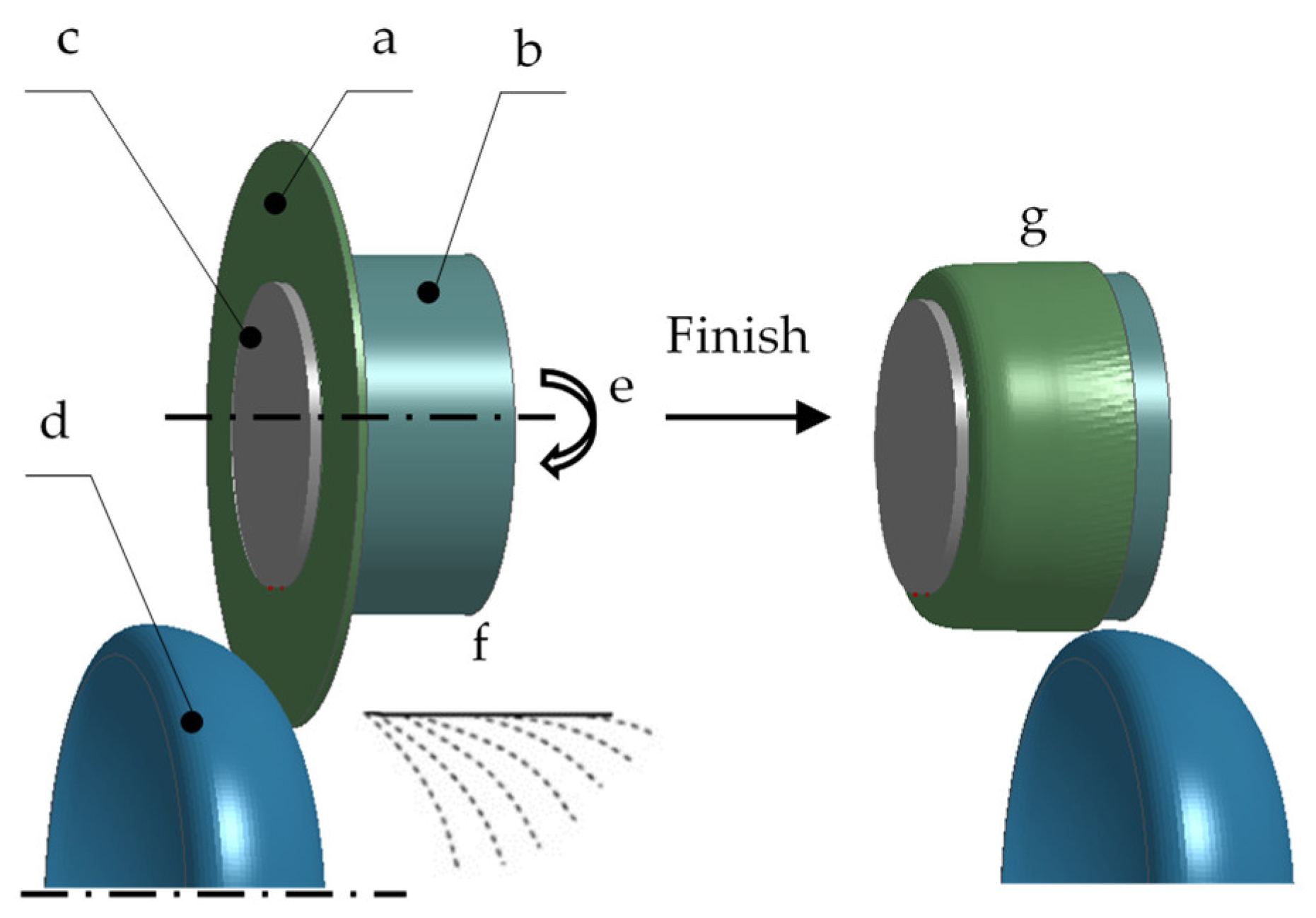
Metal spinning is the process of forming a circular plate or disc into an axisymmetric shape with a mandrel. The elementary components of the process, shown in Figure 1, include the following: a circular plate to be formed, a rotating mandrel, a backplate for clamping the plate to the mandrel, and a forming tool or roller. The simultaneous combination of roller paths and mandrel rotational speed forms the initial flat plate into an axisymmetric shape over the mandrel.

Over the past few decades, the numerical method based on dynamic finite element (FE) analysis has been used to compute almost every output of the process, allowing for the prediction of the stresses, strains, deformed geometry, and tool forces. Music et al. [1] produced an excellent review of the numerical methods used to simulate the spinning process up to 2010. They began with three studies of simplified 2D models with an assumption of axisymmetric deformation [2,3,4]. This model had a very short computational time but poor accuracy. Next, they covered nine full 3D models. These 3D models are mainly differentiated by their solvers or software (MSC [5,6], Abaqus [7,8,9], LS-Dyna [10]), their element types (solid [5,7,8], shell [9,10], or thick shell [11]), their incorporation of the strain-hardening material law (the Hollomon law [9,11], power law [7], or of the Ghosh law [10]), and their time integration schemes (implicit [12] or explicit [5,7,9,10]). One article [13] integrated the generalized incremental stress state-dependent damage model (GISSMO) into a numerical simulation of the process to predict the circumferential cracking defect by measuring a damaged scalar D in which failure occurred at $D=1$.

Figure 1. Metal spinning process components: (a) circular plate, (b) mandrel, (c) backplate, (d) roller, (e) rotating mandrel, (f) roller paths, and (g) final part [14].

Figure 1. Metal spinning process components: (a) circular plate, (b) mandrel, (c) backplate, (d) roller, (e) rotating mandrel, (f) roller paths, and (g) final part [14].

The disadvantage of these conventional 3D models is that they require an excessive amount of computational time to perform a single roller path. Therefore, these models may not be practical in predicting the final shape of a product or for optimizing a roller path where numerous tool paths are required to form a product. Some observations related to computational time are given below.

Firstly, a widely accepted assumption is that the only deformable part in the spinning process is the plate. The remaining parts, including the roller, backplate, and mandrel, are considered rigid bodies. Therefore, most of the time is invested in the plate as the rigid bodies require much less time to compute.

Secondly, the plate in the spinning process is rotating at a high speed. If there was only a rotating plate in the process without any contact with the mandrel or the roller, this would be a rotating disc problem [14], which could be modeled as a static problem in a rotating reference frame where the plate is fixed, and the rotating speed is converted to a centrifugal force.

Based on treating the plate as a rotating disc problem, a new model, presented in this article, is configured in commercial simulation software, LS Dyna. By default, this software does not explicitly support the configuration of the spinning process in a rotating reference frame. Therefore, the strong form of the spinning process must be formulated in the rotating reference frame. The mandrel movement, the plate boundary condition, and the roller path must all be adapted to this new frame. The advantages of this configuration compared to the conventional configuration are discussed later in terms of its ability to obtain better accuracy and reduce the computational time required. The thickness distribution results are compared to the experiment and a conventional numerical model. Two new techniques are proposed for this model to obtain a convergent and accurate result with a shorter computing time.

Li et al. [6], Abd-Alrazzaq et al. [15], and Xia et al. [16] studied the influential parameters of the spinning process via experiments using a computer numerical control (CNC) machine. They first presented the most significant parameters and then explained how they optimized those parameters for the minimum radial spinning force and tangential spinning force, which are considered to represent maximum spinning efficiency. The optimum procedure was achieved by using a large number of roller passes at a high speed ratio. Most of the parameters were investigated, but all three works use the same roller path.

Watson et al. [17,18] investigated wrinkling failure mechanics through the use of finite element simulation. The plastic hinge on the flange initiates wrinkling failure. At wrinkling initiation, the magnitude of the bending moment and the elastic strain energy are lower.

Kong et al. [11] found two stable compressive stress rings on the flange. The first one is distributed at the roller location, and the second is at the middle of the flange. The second stress ring is likely the cause of flange wrinkling. Therefore, a double-curved surface representing the outer flange, known as the buckling prediction model, which is based on the energy method, can be used to predict severe flange wrinkling. The average compressive stresses calculated in the FEM model and in the buckling model are compared to detect wrinkling defects.

Kong et al. [19] found that the compressive stress on the outer edge causes a slight wrinkling defect, which has little effect on the quality of the final part and can be smoothed out. However, the compressive stress on the inner part causes a severe wrinkling defect, which is not able to be recovered.

Chen et al. [20] proposed an analytical wrinkling defect model based on the fact that the flange diameter is reduced and its volume is consistent throughout the spinning process. Therefore, the strain and the stress of the flange can be calculated analytically without the need for an FEM model. Subsequently, the wrinkling defect is detected through a comparison of this stress to the critical circumferential stress.

Chen et al. [21] found that the specific zone affected by the roller causes the flange to wrinkle in that zone instead of the whole flange. The authors proposed a theoretical model of the annular sector instead of the annular plate.

Li et al. [22] proposed an analytical model integrating a toolpath design for wrinkle prediction. The wrinkling wave function, defined with a deforming depth variable, combined with the consistent volume, helps to calculate the critical stress that indicates wrinkle initiation. Therefore, this approach does not require a finite element method (FEM) model.

The wrinkling mechanism is caused by excessive circumferential stress on the flange. Most of the studies considered that the complete flange circumferential stress is the cause of wrinkling. However, one researcher [21] observed that only one section of the flange influences this defect.

While the roller path can be designed by using the wrinkling predictive model with the objective of avoiding wrinkle initiation, a minor wrinkle flange can be smoothed out, as observed by [19,22]. Some prediction models show that a higher forming depth can be used to avoid wrinkling [22]. Therefore, the idea that a wrinkle can be eliminated after wrinkle initiation can be a possible option for roller path design.

This paper presents an investigation of flange wrinkling after wrinkle initiation and is composed of two parts:

• A robust FEM model presents the formal transformation from the inertial frame to the rotating reference frame. This new mathematical approach is successfully applied in the simulation of the metal spinning process. In addition, new techniques related to the FEM configuration are presented, including mesh sizing based on a minimized aspect ratio, a mesh convergence study, and a feed rate scale.
• Post-wrinkle initiation is investigated by studying the wave geometry of the flange. The relationship between the wave’s parameters is presented first, followed by a verification using three different intermediate paths.

2. Spinning Process Model in a Rotating Reference Frame

2.1. Formation of a Plate in a Rotating Frame

The equation of motion in an inertial frame is written as

$$\frac{\partial {\sigma }_{ij}}{\partial x_j}+b_i=\rho a_i$$

(1)

in which $ij$ is the Einstein notation,

${\sigma }_{ij}$ are stresses,

$b_i$ are the body forces,

$a_i$ are accelerations, and

$\rho$ is the density.

These parameters are expressed in an inertial frame, but while the stresses σ and density $\rho$ are independent of the frame, the two other parameters, accelerations a and body forces b are dependent on the reference frame. In the spinning process, the body forces, which are caused by gravity, can be neglected. Therefore, acceleration is the only parameter that needs to be derived in the rotational frame. The acceleration is the derivative of velocity with respect to time, and velocity is the derivative of displacement with respect to time; the displacement, velocity and acceleration therefore need to be derived in order.

Figure 2 shows an arbitrary point P on the plate in the inertial frame ${\mathcal{F}}_0$ and in the rotational frame ${\mathcal{F}}_1$. The velocity and acceleration of this point are calculated in the rotational frame ${\mathcal{F}}_1$ from the inertial frame ${\mathcal{F}}_0$, as shown below.

Point $P$ on the plate is described by a vector ${\left(\overrightarrow{r_p}\right)}_{{\mathcal{F}}_0}$ in the inertial frame and by a vector ${\left(\overrightarrow{r_p}\right)}_{{\mathcal{F}}_1}$ in the rotational frame. Two vectors are related by the vector connecting two frames ${\overrightarrow{r}}_A$

$${\left(\overrightarrow{r_p}\right)}_{{\mathcal{F}}_0}={\overrightarrow{r}}_A+{\left(\overrightarrow{r_p}\right)}_{{\mathcal{F}}_1}$$

(2)

The velocity of a point in the inertial frame ${\overrightarrow{v}}_{{\mathcal{F}}_0}$ is the derivative versus time of its position.

$$\begin{array}{cc}{\left({\overrightarrow{v}}_p\right)}_{{\mathcal{F}}_0}=\frac{d}{dt}\left({\left(\overrightarrow{r_p}\right)}_{{\mathcal{F}}_0}\right)& =\frac{d}{dt}\left({\overrightarrow{r}}_A+{\left(\overrightarrow{r_p}\right)}_{{\mathcal{F}}_1}\right)\\ & =\underset{=0}{\underbrace{\frac{d}{dt}\left({\overrightarrow{r}}_A\right)}}+\frac{d}{dt}{\left(\overrightarrow{r_p}\right)}_{{\mathcal{F}}_1}\end{array}$$

(3)

When the position between two frames is fixed, then the derivative of vector $\frac{d}{dt}\left({\overrightarrow{r}}_A\right)=0$. Hence, the only unknown term is the derivative of the position $P$ versus time $\frac{d}{dt}{\left(\overrightarrow{r_p}\right)}_{{\mathcal{F}}_1}$. The vector ${\left(\overrightarrow{r_p}\right)}_{{\mathcal{F}}_1}$ can be decomposed according to a unit vector referenced in the rotational frame.

$${\left(\overrightarrow{r_p}\right)}_{{\mathcal{F}}_1}=p_x\overrightarrow{e_x}+p_y\overrightarrow{e_y}+p_z\overrightarrow{e_z}$$

(4)

Taking the derivative of Equation (4)

$${\frac{d}{dt}\left(\overrightarrow{r_p}\right)}_{{\mathcal{F}}_1}=\underset{{\left({\overrightarrow{v}}_p\right)}_{{\mathcal{F}}_1}}{\underbrace{{\dot{p}}_x \overrightarrow{e_x}+{\dot{p}}_y\overrightarrow{e_y}+{\dot{p}}_z\overrightarrow{e_z}}}+\underset{\overrightarrow{\omega }\times {{\left({\overrightarrow{r}}_p\right)}_{\mathcal{F}}}_1}{\underbrace{p_x\overrightarrow{{\dot{e}}_x}+p_y\overrightarrow{{\dot{e}}_y}+p_z\overrightarrow{{\dot{e}}_z}}},$$

(5)

and then substituting Equation (5) in Equation (3), the relationship between the velocities described in the two different reference frames ${\mathcal{F}}_0$ and ${\mathcal{F}}_1$ can be written as

$${\left({\overrightarrow{v}}_p\right)}_{{\mathcal{F}}_0}={\left({\overrightarrow{v}}_p\right)}_{{\mathcal{F}}_1}+\overrightarrow{\omega }\times {{\left({\overrightarrow{r}}_p\right)}_{\mathcal{F}}}_1$$

(6)

where $\overrightarrow{\omega }$ is the angular velocity vector.

The last step is the derivation of the expression of the acceleration:

$$\begin{array}{cc}{\left({\overrightarrow{a}}_p\right)}_{{\mathcal{F}}_0}& =\frac{d}{dt}\left({\left({\overrightarrow{v}}_p\right)}_{{\mathcal{F}}_1}+\overrightarrow{\omega }\times {{\left({\overrightarrow{r}}_p\right)}_{\mathcal{F}}}_1\right)\hfill \\ & =\frac{d}{dt}\left({\left({\overrightarrow{v}}_p\right)}_{{\mathcal{F}}_1}\right)+\frac{d}{dt}\left(\overrightarrow{\omega }\times {{\left({\overrightarrow{r}}_p\right)}_{\mathcal{F}}}_1\right)\hfill \\ & =\frac{d}{dt}\left({\left({\overrightarrow{v}}_p\right)}_{{\mathcal{F}}_1}\right)+\overrightarrow{\alpha }\times {{\left({\overrightarrow{r}}_p\right)}_{\mathcal{F}}}_1\hfill \\ & +\overrightarrow{\omega }\times \frac{d}{dt}\left({{\left({\overrightarrow{r}}_p\right)}_{\mathcal{F}}}_1\right)\hfill \end{array}$$

(7)

in which $\overrightarrow{\alpha }$ is the angular acceleration vector. The last term was calculated using Equation (5), and so the only remaining unknown term is the first one $\frac{d}{dt}\left({{\left({\overrightarrow{v}}_p\right)}_{\mathcal{F}}}_1\right)$. The velocity of a point $P$ in rotating frame ${\left({\overrightarrow{v}}_P\right)}_{{\mathcal{F}}_1}$ can be decomposed using a unit vector:

$${\left({\overrightarrow{v}}_P\right)}_{{\mathcal{F}}_1}={\dot{p}}_x\overrightarrow{e_x}+{\dot{p}}_y\overrightarrow{e_y}+{\dot{p}}_z\overrightarrow{e_z}$$

(8)

Next, we take a derivative of Equation (8)

$$\frac{d}{dt}{\left({\overrightarrow{v}}_P\right)}_{{\mathcal{F}}_1}=\underset{{\left({\overrightarrow{a}}_P\right)}_{{\mathcal{F}}_1}}{\underbrace{{\ddot{p}}_x \overrightarrow{e_x}+{\ddot{p}}_y\overrightarrow{e_y}+{\ddot{p}}_z\overrightarrow{e_z}}}+\underset{\overrightarrow{\omega }\times {{\left({\overrightarrow{v}}_P\right)}_{\mathcal{F}}}_1}{\underbrace{{\dot{p}}_x\overrightarrow{{\dot{e}}_x}+{\dot{p}}_y\overrightarrow{{\dot{e}}_y}+{\dot{p}}_z\overrightarrow{{\dot{e}}_z}}}$$

(9)

By substituting Equations (5) and (9) into Equation (7), the relationship of the accelerations between two frames can be written as

$${\left({\overrightarrow{a}}_p\right)}_{{\mathcal{F}}_0}={\left({\overrightarrow{a}}_P\right)}_{{\mathcal{F}}_1}+2\overrightarrow{\omega }\times {\left({\overrightarrow{v}}_P\right)}_{{\mathcal{F}}_1}+\overrightarrow{\alpha }\times {\left({\overrightarrow{r}}_P\right)}_{{\mathcal{F}}_1}+\overrightarrow{\omega }\times \left(\overrightarrow{\omega }\times {\left({\overrightarrow{r}}_P\right)}_{{\mathcal{F}}_1}\right)$$

(10)

Finally, the equation of motion becomes

$$\frac{\partial {\sigma }_{ij}}{\partial x_j}=\rho \left({\left({\overrightarrow{a}}_P\right)}_{{\mathcal{F}}_1}+2\overrightarrow{\omega }\times {\left({\overrightarrow{v}}_P\right)}_{{\mathcal{F}}_1}+\overrightarrow{\alpha }\times {\left({\overrightarrow{r}}_P\right)}_{{\mathcal{F}}_1}+\overrightarrow{\omega }\times \left(\overrightarrow{\omega }\times {\left({\overrightarrow{r}}_P\right)}_{{\mathcal{F}}_1}\right)\right)$$

(11)

The vector quantities and the location of the point $P$ are now represented in the rotating frame ${\mathcal{F}}_1$. There are three new terms: the Coriolis force $2\overrightarrow{\omega }\times {\left({\overrightarrow{v}}_P\right)}_{{\mathcal{F}}_1}$, the Euler force $\overrightarrow{\alpha }\times {\left({\overrightarrow{r}}_P\right)}_{{\mathcal{F}}_1}$ and the centrifugal force $\overrightarrow{\omega }\times \left(\overrightarrow{\omega }\times {\left({\overrightarrow{r}}_P\right)}_{{\mathcal{F}}_1}\right)$.

2.2. Formulation of the New Tool Path in the Rotating Frame

The roller is modeled as a rigid body. Therefore, the roller path is described by its center point. The displacement of this point is the difference between two locations at two instants $t$ and $t_0$ and is written as

$${\overrightarrow{u}}_{{\mathcal{F}}_1}^{\left(t\right)}={\overrightarrow{r}}_{{\mathcal{F}}_1}^{\left(t\right)}-{\overrightarrow{r}}_{{\mathcal{F}}_1}^{\left(t_0\right)}$$

(12)

These two terms expressed in the rotating frame can be described in the inertial frame ${\mathcal{F}}_0$ as

$${\overrightarrow{r}}_{{\mathcal{F}}_1}^{\left(t\right)}=\stackrel{=}{R}{\overrightarrow{r}}_{{\mathcal{F}}_0}^{\left(t\right)}$$

(13)

where $\stackrel{=}{R}$ is the rotational matrix

$$\stackrel{=}{R}=\left[\begin{array}{ccc}cos\omega t& sin\omega t& 0\\ -sin\omega t& cos\omega t& 0\\ 0& 0& 1\end{array}\right]$$

(14)

The initial location in frame ${\mathcal{F}}_1$ can be chosen so that the two frames have the same origin. Therefore, ${\overrightarrow{r}}_{{\mathcal{F}}_1}^{\left(t_0\right)}={\overrightarrow{r}}_{{\mathcal{F}}_0}^{\left(t_0\right)}$. Finally, the displacement formula of the roller can be transferred to the rotating reference frame, as expressed below.

$${\overrightarrow{u}}_{{\mathcal{F}}_1}^{\left(t\right)}=\stackrel{=}{R}{\overrightarrow{r}}_{{\mathcal{F}}_0}^{\left(t\right)}-{\overrightarrow{r}}_{{\mathcal{F}}_0}^{\left(t_0\right)}$$

(15)

3. Finite Element Model of a New Spinning Approach in LS-DYNA

3.1. Inefficiency of the Rotating Boundary Condition of a Plate in a Conventional Configuration

The most common approach to reduce computational time, i.e., via a larger time step size, is to assume that the process is quasi-static so that two techniques, mass scaling and loading rate scaling, can be applied to maintain the quasi-static status that can be respected if the ratio of kinetic energy to internal energy is less than 10% and the impact tool speed is less than 1% of the material dilatational wave speed [23].

The dilatational wave speed is

$$V_d=\sqrt{\frac{E\left(1-\nu \right)}{\left(1+\nu \right)\left(1-2\nu \right)\rho }}$$

(16)

in which $E$ is the elasticity modulus,

$\nu$ is Poisson’s ratio, and

$\rho$ is the density.

There are two places of contact in the spinning process, the speed of the rotational boundary condition $V_c$ and the speed of the impact between the roller and the plate $V_z$. Therefore, the scaling is limited by two conditions, $C_1$ and $C_2$, for $V_c$ and $V_z$, respectively.

The speed of the rotational boundary condition $V_c$ is also called the circumferential speed of the inner radius of the plate, as shown in Figure 3, and given below in Equation (17).

$$V_c=2\pi R_{in}\times \frac{\omega }{60\times 1000} (\mathrm{m}/\mathrm{s})$$

(17)

The other condition is the speed of the impact between the roller and the plate $V_z$. The roller slides on the surface of the plate in the circumferential direction and in the radial direction; hence, the effect of the roller on the plate in the circumferential direction is neglected because a very small friction effect occurs as the roller is rotating around its own axis. The only noteworthy speed is in the stroke or z direction. The speed of this stroke is calculated by the rotating speed $\omega$ (rpm) multiplied by the feed rate $f$ (mm/rev), as shown in Equation (18).

$$V_z=\frac{\omega }{60}\times \frac{f}{1000}(\mathrm{m}/\mathrm{s})$$

(18)

In loading-rate scaling, the rotating speed of the mandrel $\omega$ is scaled up by a multiplier $\alpha$ to become the artificial rotating speed ${\omega }_a=\alpha \omega$. Therefore, the rotational speed artificially becomes $V_{ca}=\alpha V_c$, and the axial speed becomes $V_{za}=\alpha V_z$. The constraint that ratio of the impact speed impact speed over the dilatational speed be smaller than 1% must be respected.

The first condition of rotational speed gives a limitation $C_1$ for the multiplier $\alpha$.

$$\frac{V_{ca}}{V_d}=\alpha \frac{V_c}{V_d}<0.01⟺\alpha <0.01\frac{V_d}{V_c}=C_1$$

(19)

The second condition of stroke speed gives the limitation $C_2$ for the same multiplier $\alpha$.

$$\frac{V_{za}}{V_d}=\alpha \frac{V_z}{V_d}<0.01⟺\alpha <0.01\frac{V_d}{V_z}=C_2$$

(20)

Therefore, the multiplier $\alpha$ is either smaller than $C_1$ or smaller than $C_2$.

The ratio $\frac{C_2}{C_1}=\frac{V_c}{V_z}=\frac{2\pi R_{in}}{f}$. In practice, the feed rate is often less than 1 $\mathrm{m}\mathrm{m}/\mathrm{r}\mathrm{e}\mathrm{v}$ to reduce the wrinkles, and the radius $R_{in}$ depends on the dimension of the mandrel, which is usually larger than 1 mm. Therefore, the ratio $\frac{2\pi R_{in}}{f}$ is larger than 1 and so the condition $C_2$ is larger than condition $C_1$, by $\frac{2\pi R_{in}}{f}$ times.

The potential increase in loading rate scaling is limited by the first condition $C_1$ in the case of a conventional model. In contrast, the new model does not have that first condition, and so the loading rate scaling can be applied as the value of condition $C_2$, which is much larger than that of condition $C_1$.

In mass scaling, the mass is scaled up by a multiplier $\beta$ so the artificial density ${\rho }_a=\beta \rho$, or reducing dilatational speed.

$$V_{da}=\frac{V_d}{\sqrt{\beta }}$$

(21)

The first condition of rotational speed gives a limitation $C_1$ for the multiplier $\beta$,

$$\frac{V_c}{V_{da}}=\frac{V_c}{V_d}\sqrt{\beta }<0.01⟺\beta <{\left(0.01\frac{V_d}{V_c}\right)}^2=C_1$$

(22)

while the second condition of stroke speed gives a limitation $C_2$ for the multiplier $\beta$.

$$\frac{V_z}{V_{da}}=\frac{V_z}{V_d}\sqrt{\beta }<0.01⟺\beta <{\left(0.01\frac{V_d}{V_z}\right)}^2=C_2$$

(23)

Therefore, the multiplier $\beta$ is either smaller than $C_1$ or smaller than $C_2$.

The ratio $\frac{C_2}{C_1}={\left(\frac{V_c}{V_z}\right)}^2={\left(\frac{2\pi R_{in}}{f}\right)}^2$, and so the condition $C_2$ is larger than condition $C_1$, by ${\left(\frac{2\pi R_{in}}{f}\right)}^2$ times.

The potential increase in mass scaling may also be limited by the first condition $C_1$ in the case of a conventional model. In contrast, the new model does not have the first condition, and so the mass scaling can be applied as long as condition $C_2$ is much larger than condition $C_1$.

3.2. Boundary Condition

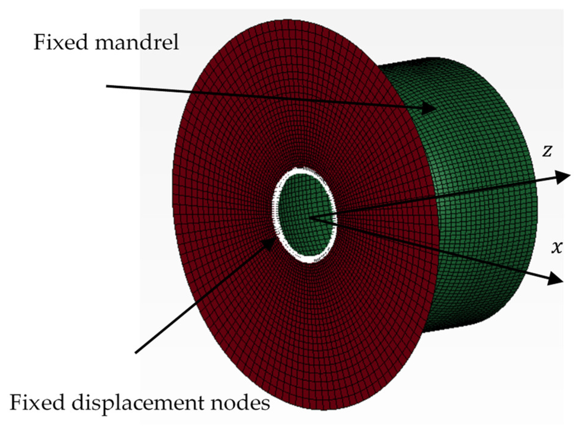
Based on the previous derivation of the strong form in the rotating reference frame, the mandrel and the backplate will be fixed. Therefore, the backplate does not need to be modeled and can be replaced by a fixed displacement of nodes at the outer diameter of the backplate, as shown in Figure 4. These nodes are fixed by using a LS-DYNA command “BOUDARY_SPC_SET” for six degrees of freedom x, y, z, r_x, r_y, and r_z.

The rotating speed of the mandrel is constant, $\omega =const$, which means the acceleration is zero and so the Euler force is zero. The generalized body force includes centrifugal acceleration: Coriolis acceleration is applied to the plate.

The rigid body movement is applied by prescribing the “boundary_presribed_motion_rigid” LS-DYNA command with six parameters: the x, y, and z displacements and the r_x, r_y, and r_z rotations.

According to Equation (15), there is an advantage when choosing the center of the roller so that it lies on the x-z plane where the y axis is zero. The explicit formula can be written in the matrix form.

$${\overrightarrow{u}}_{{\mathcal{F}}_1}^{\left(t\right)}=\left[\begin{array}{c}{r}_x^{\left(t\right)}cos\omega t\\ r_x^{\left(t\right)}sin\omega t\\ r_z^{\left(t\right)}\end{array}\right]-\left[\begin{array}{c}{r}_x^{\left(0\right)}\\ 0\\ r_z^{\left(0\right)}\end{array}\right]$$

(24)

This formula can be applied in LS-DYNA by the command “define_function”.

3.3. Material Model and Elements

The material was modeled using the plasticity power law ${\sigma }_y=k{ϵ}^n$, where k is the strength coefficient and n is the hardening exponent; both are shown in

Table 1. Mechanical properties of the aluminum alloy 2024-O.

Young’s Modulus (GPa)	$\mathbf{Poisson}’\mathbf{s} \mathbf{Ratio} \mathit{\nu }$	Yield Strength (MPa)	Strength Coefficient (MPa)	Hardening Exponent n
71.3	0.33	70.06	308.62	0.234

. In the experiment, the thickness of the final product can be 18.33% smaller than the initial thickness. Therefore, the element’s formula should include the change in thickness. A shell formula with variable thickness was chosen for the model. A full integration Gauss point was chosen because it responds very well in tensile tests compared to the reduced integration scheme, offering the same accuracy. Another advantage is that it does not require any additional element, so the time step size is a benefit of this feature. The 4-node fully integrated shell element with thickness stretch was therefore chosen, as shown in Equation (26), in LS-DYNA software.

3.4. Loading Rate Scaling

If the material in the metal spinning process can be assumed to be quasi-static and non-rate-dependent, the stroke speed of the roller can be increased without affecting the simulation results. The stroke of the roller moves in both the circumferential and z directions. The circumferential speed relates to the rotating speed. The z speed relates to the feed ratio mm/rev and the rotating speed rev/minute, so it has speed in mm/minute. Therefore, the rotating speed and/or the feed ratio can be used to increase the stroke speed. However, it is reported in the literature that the feed ratio plays an important role in flange wrinkling [11]. Therefore, only the rotating speed is used here to speed up the stroke speed with a constant feed ratio.

3.5. Mass Scaling

Mass scaling is another way to speed up the simulation time with the assumption of a quasi-static state. As the density of the material increases, the dilatational wave speed in the material decreases; hence, the stable time step size increases. The mass is added to quantify the number of elements whose characteristic length is small so that the time step size satisfies all the elements of the plate. In this way, greater mass is added to the inner surface of the plate, where the characteristic lengths of these elements are the smallest.

4. Experiment and Simulation Configuration

The proposed numerical model was validated with experiments, and its robustness was verified using common models. An experiment of the conventional spinning of a hemispherical part described in [16] was used, as well as the results of their simulation.

The aluminum alloy 2024-O circular plate with the properties listed in Table 1 has a 200 mm diameter and a 1.8 mm thickness. The mandrel speed is 200 rpm, and the feed ratio is 1 mm/rev. The process parameters and the toolpath are shown in Figure 5; a workpiece with a thickness of 1.8 mm and a roller radius of 10 mm follows the shape of the mandrel with a radius of 69.61 mm until reaching the angle of 55°.

The thickness distribution is measured when the stroke angle, which is the angle between the roller and the center axis, as shown in Figure 6, is 55°.

The elements shown along the line indicated in Figure 7 are selected to measure their thickness. The thickness of the final product was measured by using the laser scanning system.

5. Results and Discussion

5.1. Mesh Convergence Study

A reliable result is a value that is not affected by changing the size of the mesh. The response of thickness distribution will converge to a repeatable solution with decreasing element size. Therefore, one strategy is to run multiple simulations from coarse to fine mesh until a converged result is obtained.

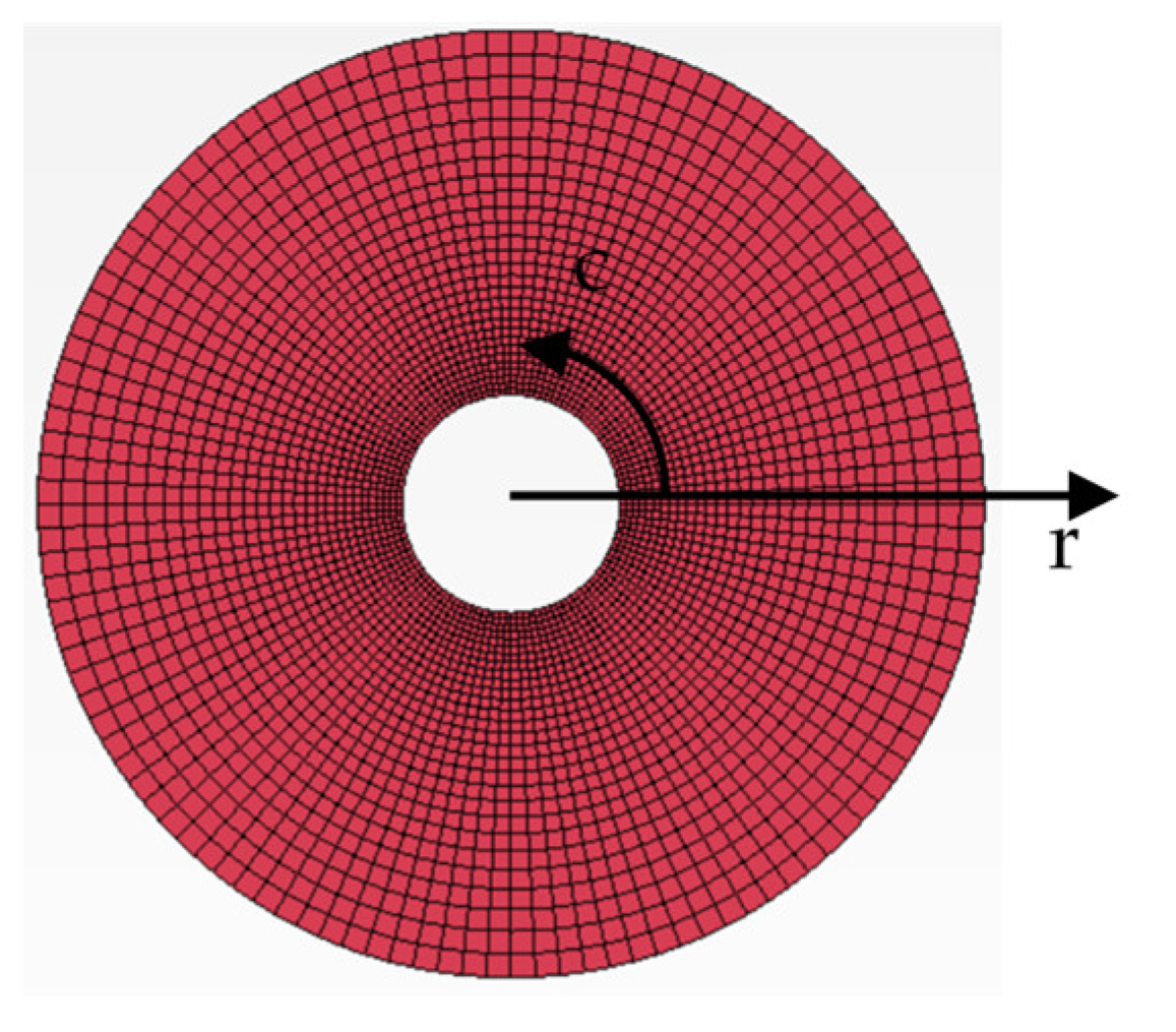
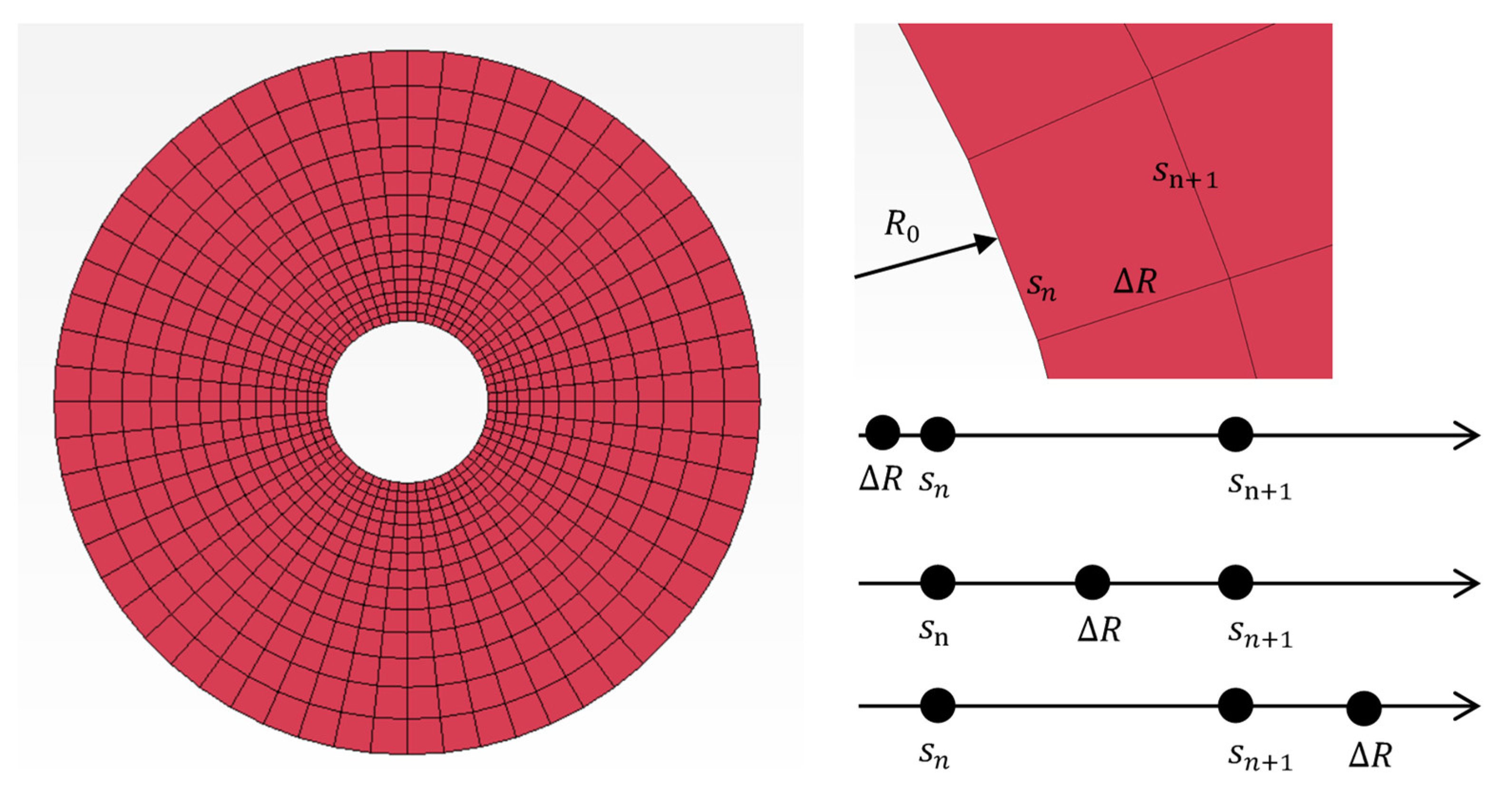
The disc can be meshed using two parameters: the number of elements in the radial direction $n_r$ and the number of elements in the circumferential direction $n_c$, as shown in Figure 8. The running strategy is simple when there is only one variable to vary instead of two, here $n_r$ and $n_c$. In this paper, the rule applied to construct a relation between $r$ and $c$ is that the aspect ratio of the mesh is always minimized. By focussing on this minimization of the mesh ratio, the solution is convergent to the final value that matches well with the experiment.

The aspect ratio is the ratio of the longest and shortest lengths of an element’s edges. Let us start with the element shown in Figure 9. It is formed by three parameters $s_n$, $\Delta R_n$ and $s_{n+1}$. The first length of the element is

$$s_n=2R_n\mathit{tan}\left(\frac{\pi }{c}\right)$$

(25)

The parameter $s_{n+1}$ can be calculated in the same manner, but with a larger radius $R_{n+1}=R_0+\Delta R$.

$$s_{n+1}=2R_{n+1}\mathit{tan}\left(\frac{\pi }{c}\right)=2\left(R_n+\Delta R_n\right)\mathit{tan}\left(\frac{\pi }{c}\right)$$

(26)

The parameter $s_{n+1}$ is always larger than $s_n$. Therefore, the parameter $\Delta R$ can fall into three possible cases: $\Delta R_n\le s_n<s_{n+1}$, $s_n<\Delta R_n<s_{n+1}$ and $s_n<s_{n+1}\le {\Delta R}_n$. This is visually represented in Figure 9 (graph on the right).

In the first case, with $\Delta R_n\le s_n<s_{n+1}$, the aspect ratio $A{S}_1=\frac{s_{n+1}}{\Delta R_n}$, so that $\underset{\Delta R_n}{\mathit{min}}A{S}_1=\frac{s_{n+1}}{s_n}=1+2\mathit{tan}\left(\frac{\pi }{c}\right)$ when $\Delta R=s_n$.

In the second case, with $s_n<\Delta R_n<s_{n+1}$, the aspect ratio $A{S}_2=\frac{s_{n+1}}{s_n}$, so that $\underset{\Delta R_n}{\mathit{min}}A{S}_2=\frac{s_{n+1}}{s_n}=1+2\mathit{tan}\left(\frac{\pi }{c}\right)$.

In the third case, with $s_n<s_{n+1}\le {\Delta R}_n$, the aspect ratio $A{S}_3=\frac{\Delta R_n}{{\mathrm{s}}_{\mathrm{n}}}$, so that $\underset{\Delta R_n}{\mathit{min}}A{S}_3=\frac{s_{n+1}}{s_n}=\frac{1}{1-2\mathit{tan}\left(\frac{\pi }{c}\right)}$ when $\Delta R=s_{n+1}$.

The values of $AS$ of the first two cases are the same, but they are smaller than the value of $AS$ in the third case and are calculated as shown below in Equation (27).

$$\frac{\underset{\Delta R_n}{\mathit{min}}A{S}_1}{\underset{\Delta R_n}{\mathit{min}}A{S}_3}=\left(1+2\mathit{tan}\frac{\pi }{c} \right)\left(1-2\mathit{tan}\frac{\pi }{c}\right)<1$$

(27)

In conclusion, the minimum aspect ratio is $1+2\mathit{tan}\frac{\pi }{c}$ when the $\Delta R_n=s_n$.

The mesh parameters can be adjusted so that the aspect ratio is satisfied. First, the dividend in the circumferential direction is chosen to be constant. The aspect ratio is then adjusted by the parameter $n_r$ and the bias factor $bf$, which is used to control the length of the elements in the radial direction.

For a given number of elements in the circumferential direction, the bias factor $bf$ relates to the growth rate $r$ and the number of elements in the radial direction $n_r$.

$$bf=r^{n_r-1}$$

(28)

The growth rate $r$ is the ratio between the length of two contiguous elements in the radial direction.

$$r=\frac{\Delta R_{n+1}}{\Delta R_n}=\frac{s_{n+1}}{s_n}=1+\frac{\Delta R_n}{R_n}=1+\frac{s_n}{R_n}=1+2\mathit{tan}\frac{\pi }{c}$$

(29)

The number of elements is related to the growth rate as shown in the equation below.

$$n_e=\sum _{i=0}^{n_c-1}{l}_1{r}^i =\frac{l_1\left(1-r^{i+1}\right)}{1-r}$$

(30)

The number of elements in the radial direction $n_r$ is calculated with Equation (30). The bias factor is calculated with Equation (28).

Finally,

Table 2. Bias factor and average aspect ratio for four different meshes.

Mesh	${\mathit{n}}_{\mathit{e}}$	Bias Factor	Aspect Ratio Average
60_14	840	4.032	1.0078
80_18	1440	3.89988	1.0385
100_24	2400	4.3166	1.0267
120_28	3360	3.966	1.0057

presents solutions from four meshes using Ansys Workbench software with parameters $n_c\_n_r$ equal to 60_14, 80_18, 100_24, and 120_28.

The simulation is speeded up by loading rate scaling of values 10,000 rpm and 20,000 rpm. The feed ratio is constant. However, in the experiment, the forces acting on the plate are calculated at a value of 200 rpm.

The thickness distribution of the loading rate scaling at 20 k rpm is shown in Figure 10. The first two meshes exhibit a large difference at about the first 10%. While the last two meshes seem to match very well, the convergent mesh for this rate scaling was finally obtained at mesh 100_24 and 120_28.

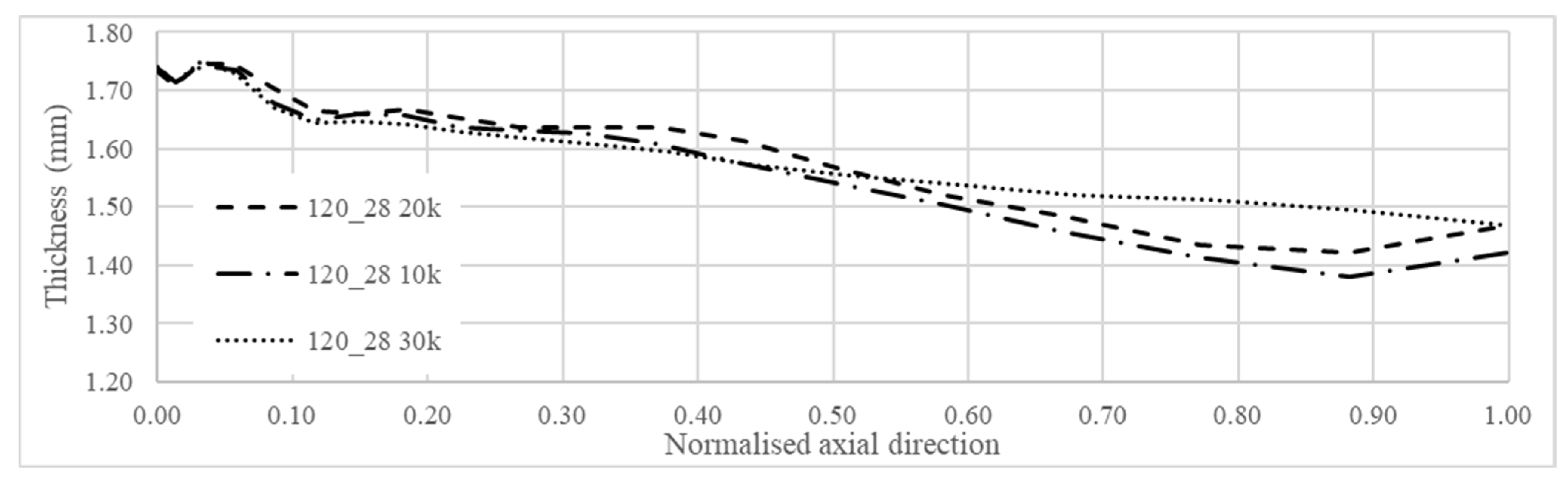
The solutions of the convergent meshes run with three different artificial rotating speeds, 10 k rpm, 20 k rpm, and 30 k rpm, are shown in Figure 11. The two curves with speeds of 10 k and 20 k are very close to each other. The curve with the speed of 30 k fits with the others until around one-third of the range, and then it diverges. Therefore, the convergent rate scaling is set at 10 k rpm.

5.2. Comparison of the Experimental Model with a Conventional Model

The thickness distribution of convergent meshes is compared to the experimental and the conventional model with the highest element number from [16], as shown in Figure 12. The maximum error between the new model and the experimental model is 7.38% at a value of 0.78.

The trend of the thickness distribution agrees well with the experiment values in the case of the new model, with four peaks: two top peaks at 0.03 and 0.16 and two bottom peaks at 0.11 and 0.878. This is not the case for the conventional model shown in Figure 12.

The maximum difference between the experiment and simulation is 0.06 mm at a normalized axial of 0.88, where the stroke angle is 55°. This value is still below the tolerance of a sheet metal thickness variation of ±0.1 mm [24].

The number of elements of the densest mesh of the conventional model is 9000, while only 3360 elements are needed for the convergent solution in the new model.

The number of elements of the densest mesh of the conventional model is 9000, while only 3360 elements are needed for the convergent solution in the new model. Furthermore, the conventional model is performed with a mass scaling of 25. This means the time step is boosted by $\sqrt{25}$ = 5 times. The new model can obtain a convergent solution at an artificial rotating speed of 10 k rpm, i.e., 50 times faster. This reveals that the computational cost of the new model is more economical than that of the conventional one in both the number of elements and scaling aspects, appropriately 12.67 times that are 10 times in terms of scaling and 2.67 times in terms of element number.

5.3. Loading Rate Scaling versus Mass Scaling

The thickness distributions of the numerical models with mass scaling and loading rate scaling are shown in Figure 13. The two curves representing the numerical results match almost all of the range, except at the beginning and near the end. A first observation is that the loading rate scaling gives a better result than mass scaling because mass scaling adds most of the mass to the inner area of the plate due to the small characteristic length of those elements. This mass produces an error of artificial added mass in this area.

Secondly, loading rate scaling has the flexibility to be applied to different stages of the process, which makes it possible to control the accuracy at any desired area.

Thirdly, mass scaling gives a convergent solution with a time step size of 7 × 10⁻⁶ for the processing time of 16.654 s; hence, the time step number is 2.379.142, while loading rate scaling has a convergent time step size of just 1.96 × 10⁻⁷ for the processing time of 0.333 s, and so its time step number is 1.698.979. The computational time of loading rate scaling is thus less than the mass scaling case by a ratio of 1 to 4.

However, loading rate scaling has a disadvantage: it cannot be applied to rate-dependent materials [23] because it changes the rate of deformation, which will affect the response stress–strain curve of the rate-dependent material.

5.4. Influence of the Rotating Speed

By analyzing the spinning process in a rotating reference frame, it can be determined that the rotating speed of the mandrel creates centrifugal force and the Coriolis force. According to [14], the maximum stresses are where centrifugal force is created on the plate, as summarized in

Table 3. Stresses in the plate with various rotating speeds.

Rotating Speed (rpm)	Radial Stress (MPa)	Circumferential Stress (MPa)
200	6.94 × 10−3	3.6 × 10−3
1000	1.73 × 10−1	9.01 × 10−2
3200	1.78	0.922

. While the yield stress of the material is 70.06 MPa, the maximum stress in the plate is 1.78 MPa at 3200 rpm or 2.54% of the yield stress. This small amount of stress has only a very small effect on the deformation of the plate.

The increased rotating speed is still in the quasi-static zone, as it is less than 1% of the wave speed of the material. The simulation with a very high stroke speed at 10,000 rpm showed very small changes in the results. Hence, the variations observed in the results when increasing the rotating speed to 3200 are very small and can be neglected.

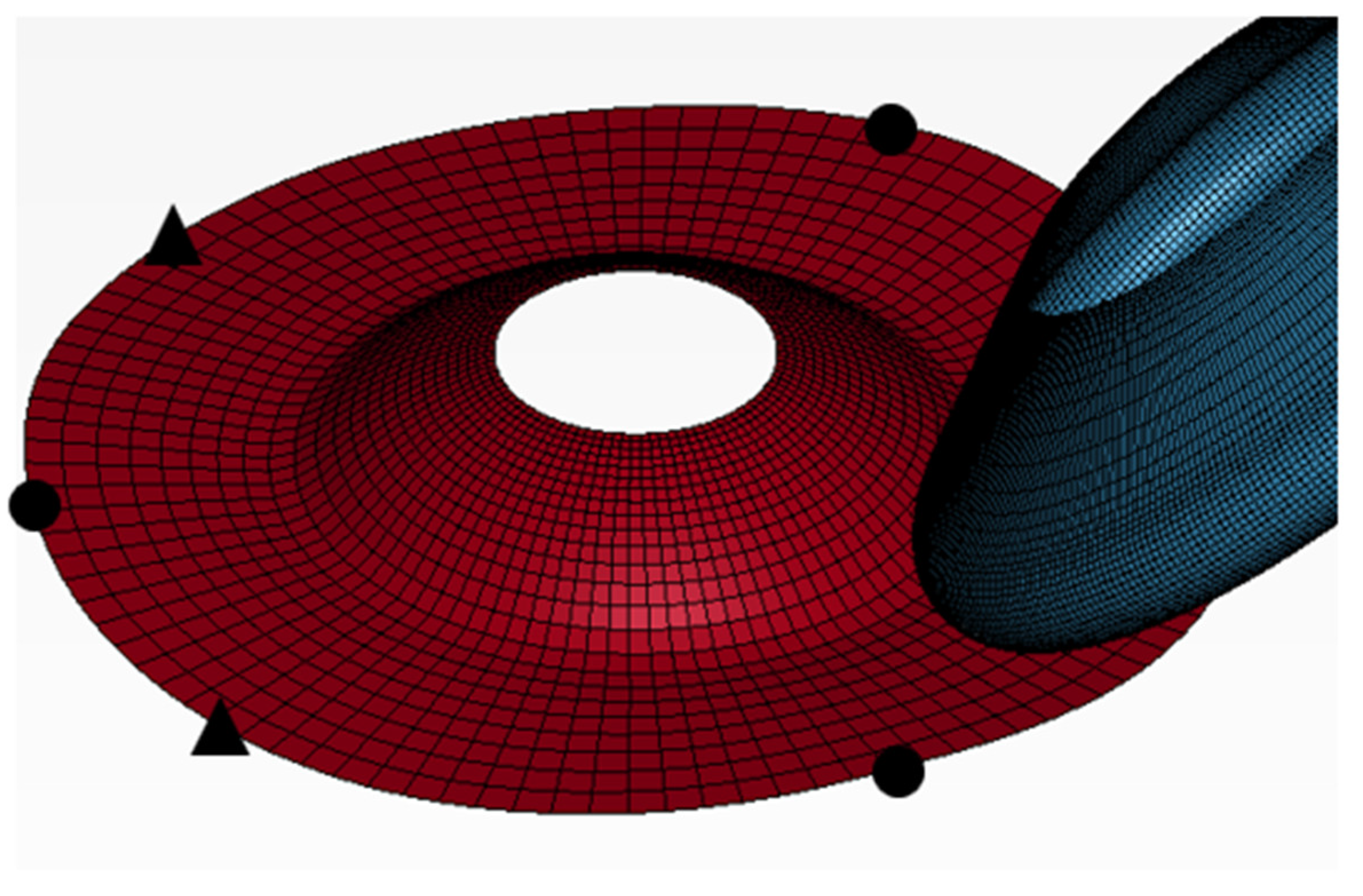
6. Post-Wrinkle Initiation Analysis

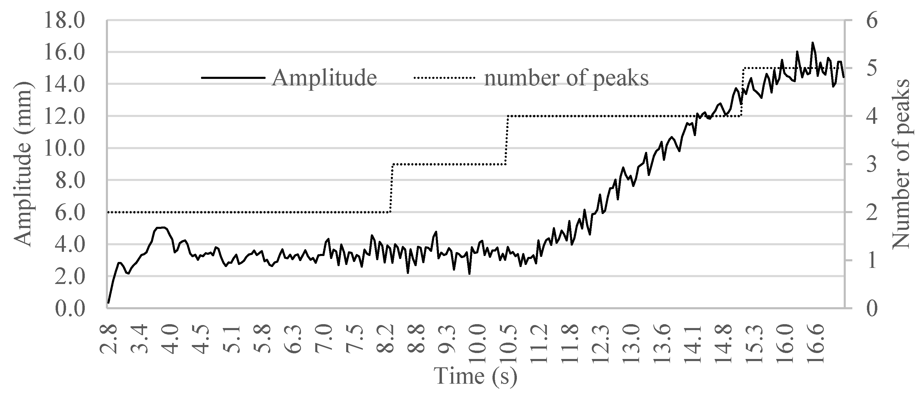
The wrinkle geometry is shown in Figure 14. It shows the wave geometry, including two main output characters: the number of peaks and the amplitude. One example of this output is shown in Figure 15. The amplitude and the number of peaks during the spinning process are shown in Figure 16. Both experiment and simulation showed that the plate begins wrinkle initiation at about 40 degrees, which occurs at 9.8 s. The wrinkle initiation can be seen on this diagram at the time of 9.8 s and corresponds to the appearance of the third peak.

The number of peaks is seen to increase from two to four, corresponding to the initial stage and severe wrinkling, respectively. In addition to the wave geometry of the flange, the hypothesis of the relationship between the number of peaks and the amplitude is proposed.

6.1. Relationship between the Number of Peaks and the Amplitude

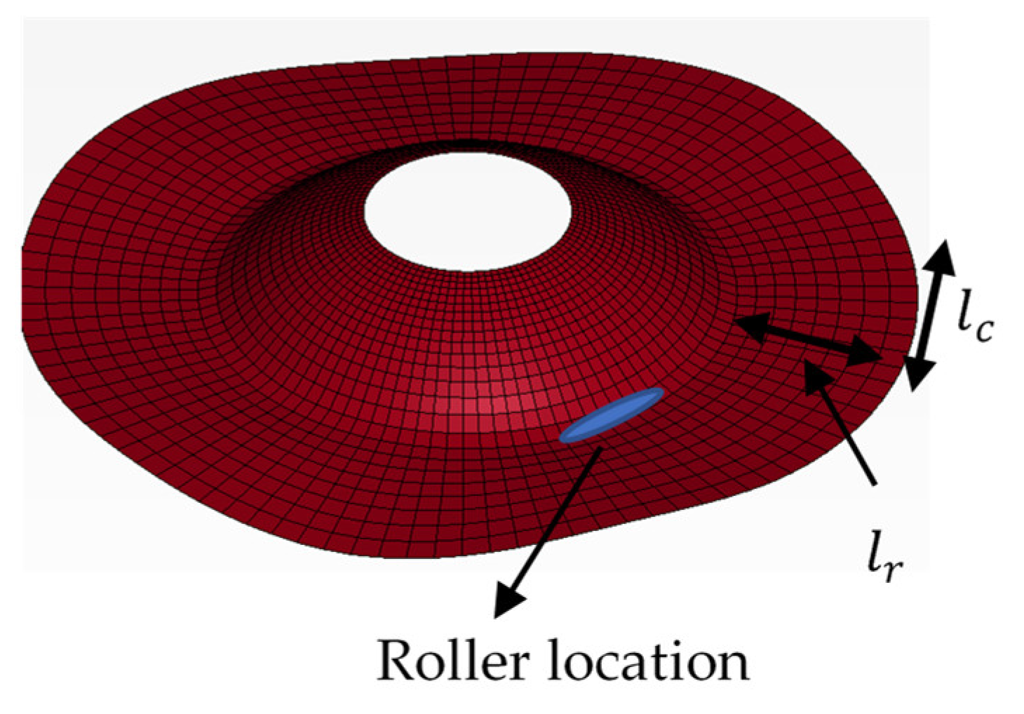
The volume of an element in the plastic deformation phase does not change for metals with a crystalline structure [25]. The initial volume of the shell element is calculated as a multiplication of its characteristic lengths, as indicated in Figure 17: radial length $l_r$, circumferential length $l_c$ and thickness t:

$$V_{elem}=l_r\times l_c\times t=constant$$

(31)

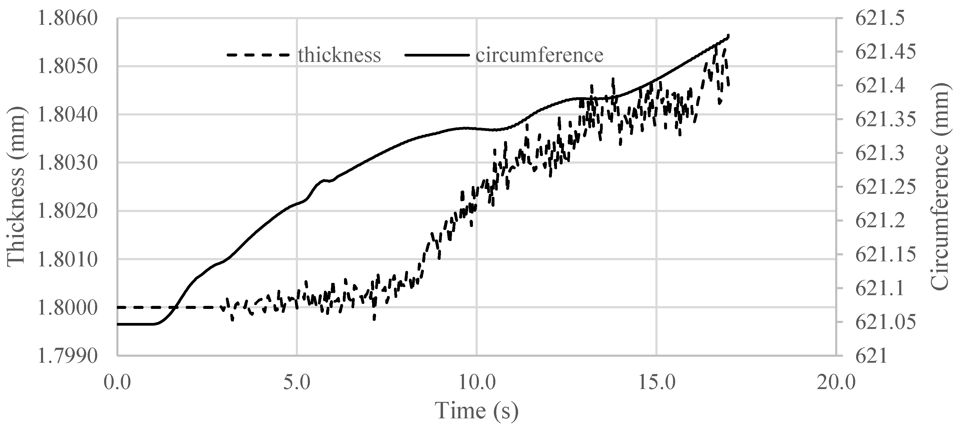
The roller deformed the plate locally at the middle of the plate, as shown in Figure 17. In addition, the flange has no constraints on the edge; hence, the thickness $t$ and the radial length $l_r$ can be considered as having little variation. The change value of the thickness and the circumference of the flange are shown in Figure 18. The thickness changes 0.3%, from 1.8 to 1.8055 mm, and the circumference changes 0.0689%, from 621.04 to 621.468 mm.

Therefore, the circumference of the flange can be considered as constant. This assumption is reasonable only until the roller deforms the edge.

Considering the wave geometry, the circumference or the length of the wave remains constant, and then the number of peaks increases, but the amplitude decreases.

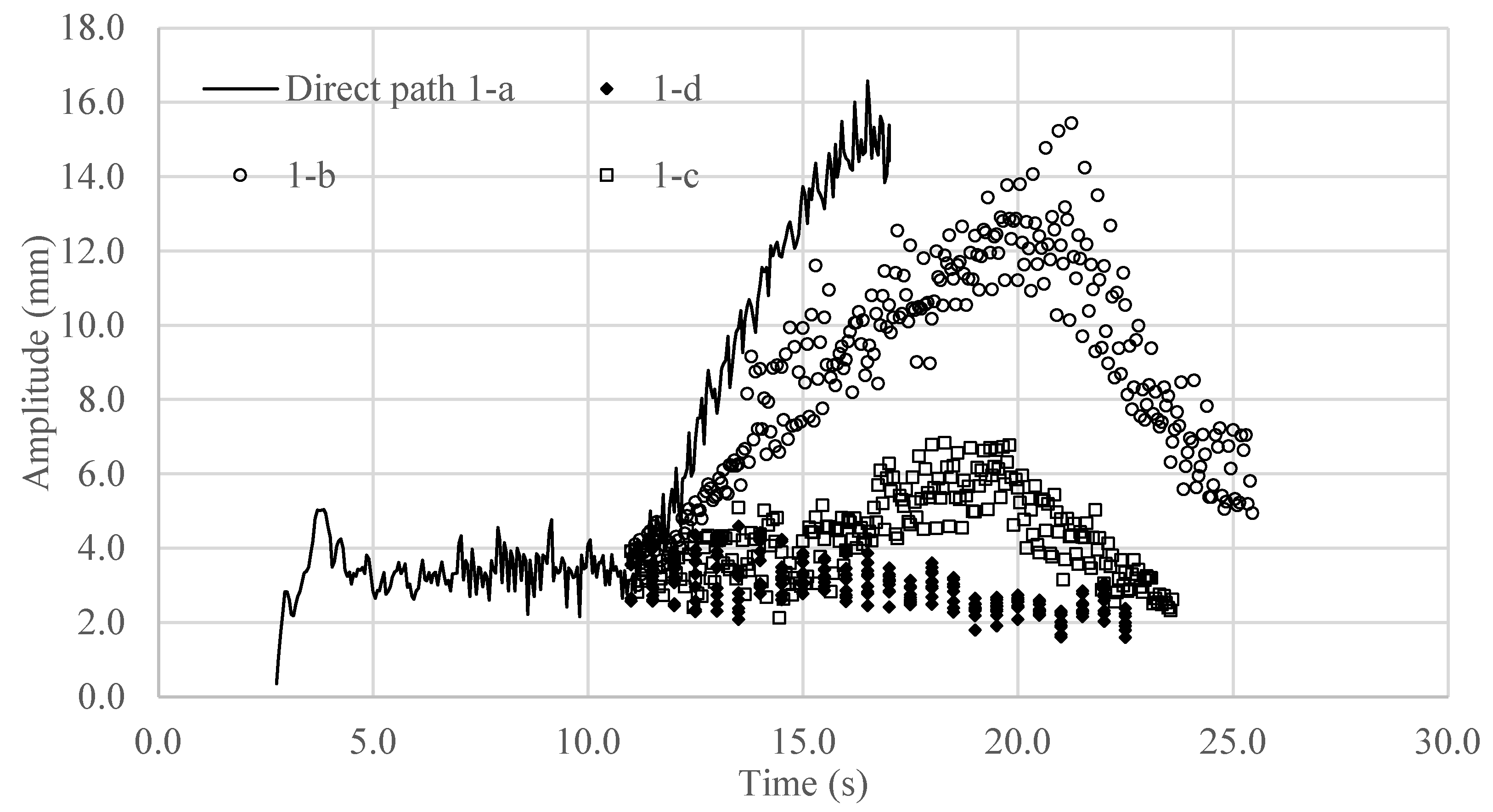
In Figure 16, when the number of peaks reaches three at time 8.25 s, the amplitude decreases. Severe wrinkling occurs at time 10.25 s when the amplitude increases suddenly with the slow growth of the number of peaks. The possibility is that the stroke angle remains large (path 1-a), as shown in Figure 19, compared to the small stroke angle of paths (1-b, 1-c, 1-d); hence, the increase in the number of peaks is not fast enough to decrease the amplitude.

Therefore, the smaller stroke angle paths called the intermediate paths are investigated to verify this hypothesis.

6.2. Investigation of 3 Intermediate Stroke Angles

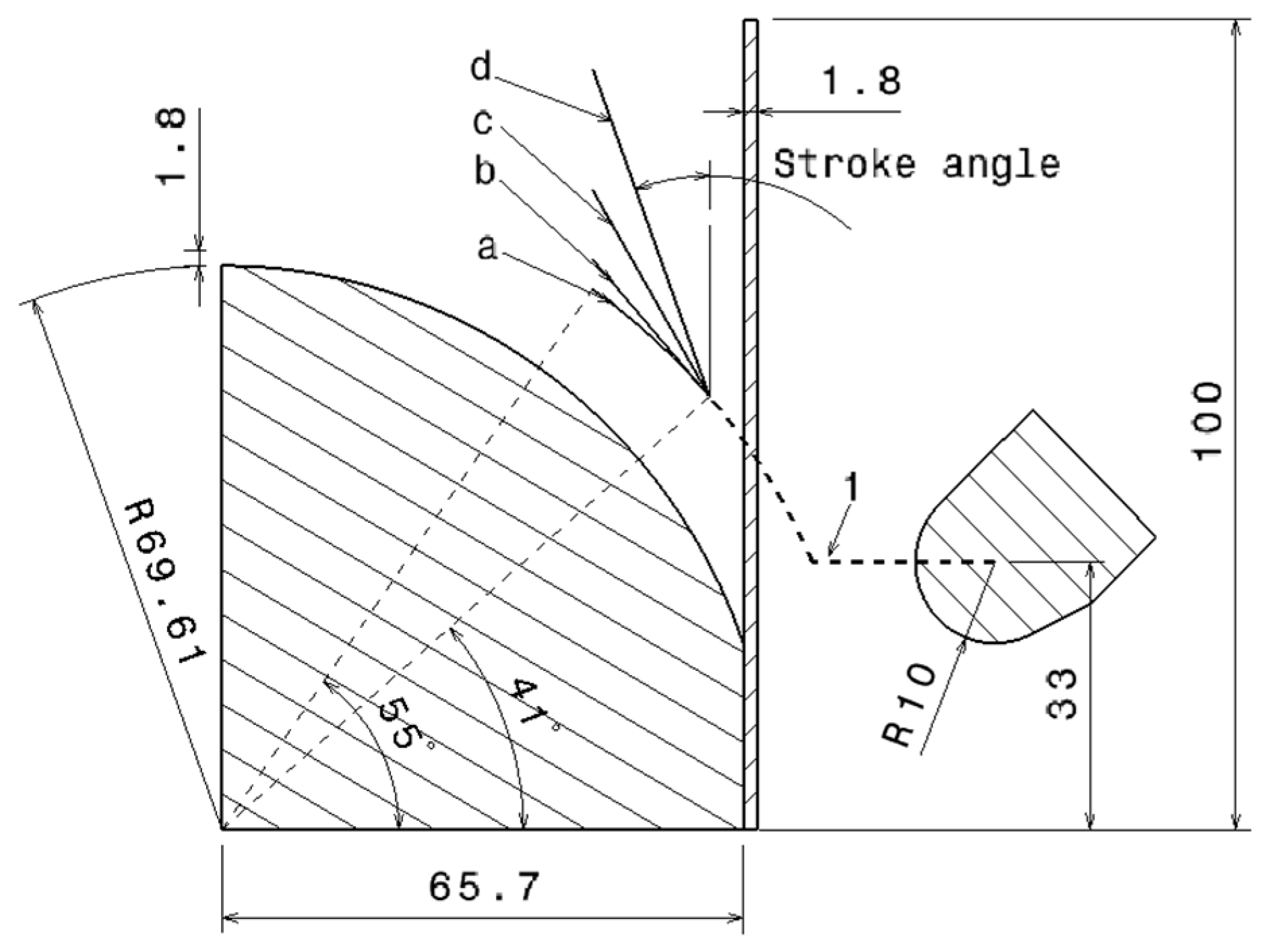
Figure 19 shows the sketch of the metal spinning process with three intermediate stroke paths. These paths start at the angle position ${41}^{\mathrm{o}}$, where the wrinkle begins. Path 1-a is the direct path used in the experiment and in the simulation in the above section. Three intermediate paths with smaller stroke angles are included: 1-b with stroke angle ${41}^{\mathrm{o}}$, 1-c with stroke angle ${30}^{\mathrm{o}}$ and 1-d with stroke angle ${20}^{\mathrm{o}}$. The amplitudes corresponding to these four cases are shown in Figure 20.

The intermediate path 1-b with a stroke angle of ${41}^{\mathrm{o}}$ showed the same trend of sudden change in amplitude as the direct path, but path 1-b results in a smaller amplitude value. At the end of the process, the amplitude of path 1-b decreases significantly to the safe value due to the increasing number of peaks, up to eight.

The intermediate path 1-c with a stroke angle of ${30}^{\mathrm{o}}$ showed growth in the amplitude in the safe range of 6 mm. The number of peaks in this path goes up to seven.

The intermediate path 1-d with a stroke angle of ${20}^{\mathrm{o}}$ showed a constant amplitude during all processes. The number of peaks remained at four. This can be considered as the best intermediate path for this process.

Finally, the second direct path must be applied in order to deform the plate to the desired location.

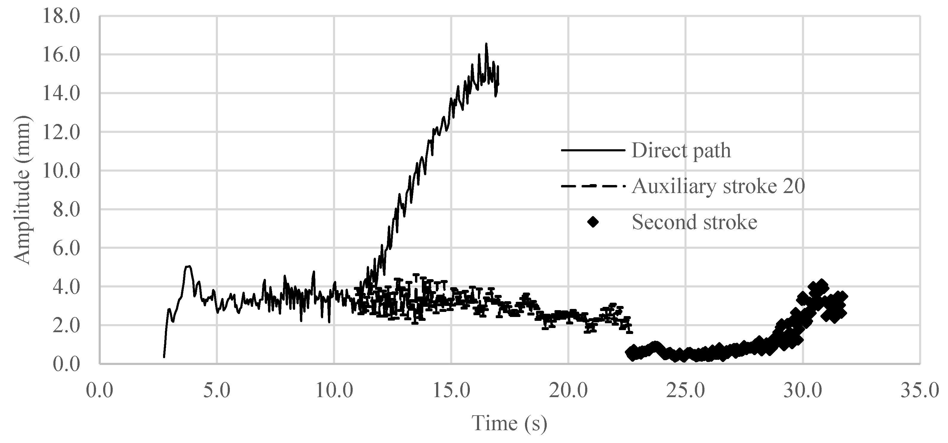
6.3. Investigation of the Second Stroke after an Intermediate Path

This section investigates the direct path from the wrinkle initiation location at ${41}^{\mathrm{o}}$ to the final location at ${55}^{\mathrm{o}}$ after utilizing the intermediate path “1-d”. The complete path is shown in Figure 21, noted as path “1-d-2”.

The amplitude of the second path “1-d-a” is shown in Figure 22. The final amplitude is about 4 mm, significantly smaller than that of the final amplitude of direct path “1-a”, 15 mm. However, the processing time of 31.65 s is longer than the 16.5 s time of the direct path “1-a” due to the intermediate path “d”.

Finally, it is shown that extra forming paths are efficient for successfully completing the spinning process but at the expense of a significant amount of processing time.

7. Conclusions

A new modeling technique was presented here, along with its supporting theory and a detailed implementation in LS-DYNA software. This technique was compared with both experimental values and the conventional model. The results obtained from the new model are in very good agreement with the experimental values. In addition, the study of the post-wrinkle initiation was investigated. The conclusions of this study are summarized below:

• The new model improves the accuracy of the thickness variation prediction in terms of value error and trend. These results showed exactly how the thickness varies throughout the final part of the spinning process, with one maximum location near the tailstock and one minimum location at the roller location. For this analysis, the computational time was 50 times faster than the conventional model. In addition, the proposed mesh pattern contributes to the accuracy and efficiency of this new model.
• Wrinkle onset can be predicted in a rotating reference frame based on the displacement of the flange.
• The amplitude and the number of peaks are related. The wrinkle can be removed by using the intermediate path, which showed that the magnitude reduces toward 2.0 while the number of maxima increases quickly toward eight. Otherwise, the number of maxima remains at four while the magnitude of the amplitude increases until it becomes defective.
• The study of three various intermediate paths reveals the potential of designing a multi-path strategy for achieving a successful metal spinning process. While the simple straight intermediate path can produce a successful process, a curved path may lead to better results, which will be investigated in the future.