
Experimental and Numerical Investigations into Heat Transfer Using a Jet Cooler in High-Pressure Die Casting

 ,
,  ,
,
Abstract
:1. Introduction
2. Materials and Methods
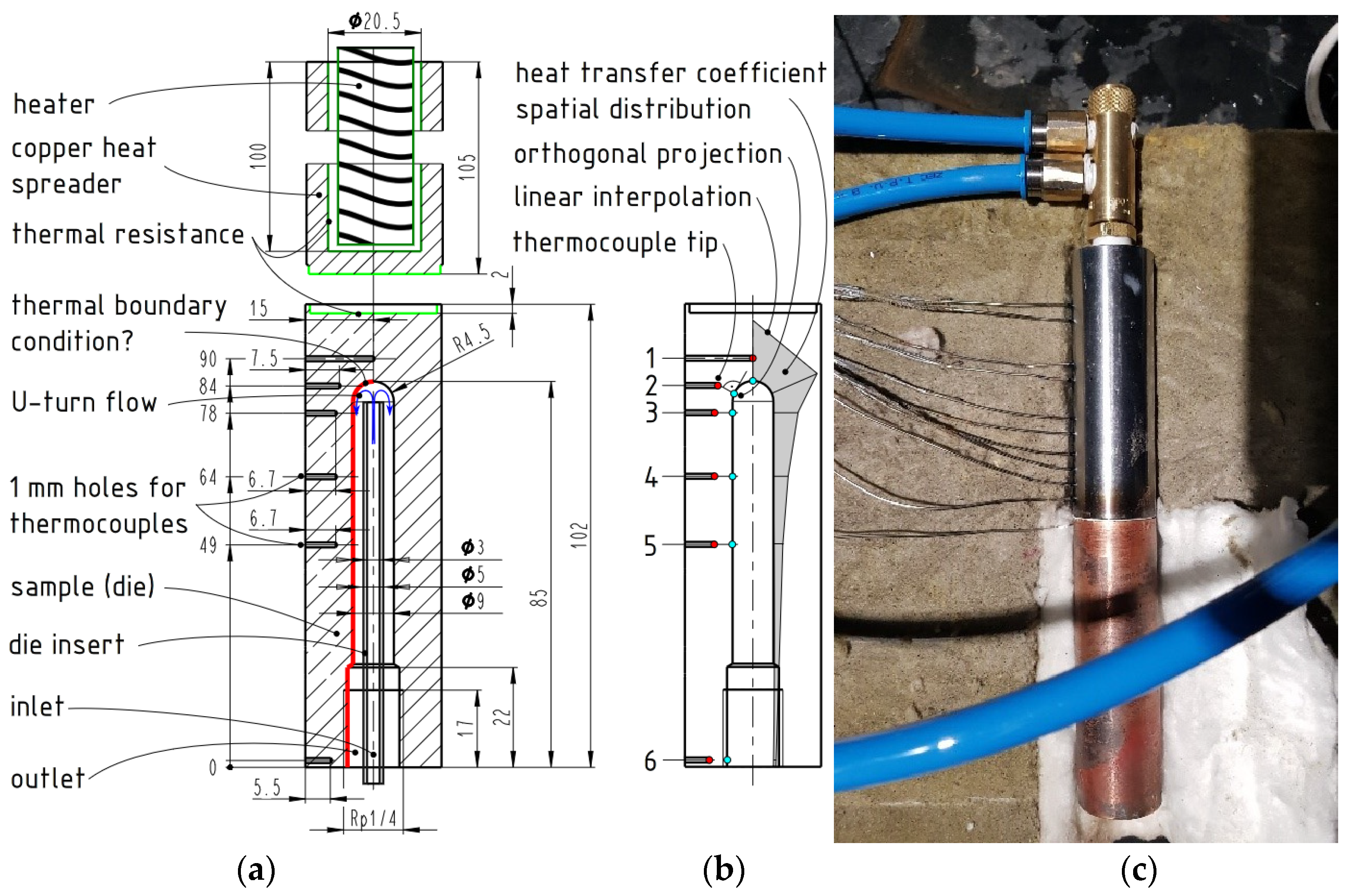
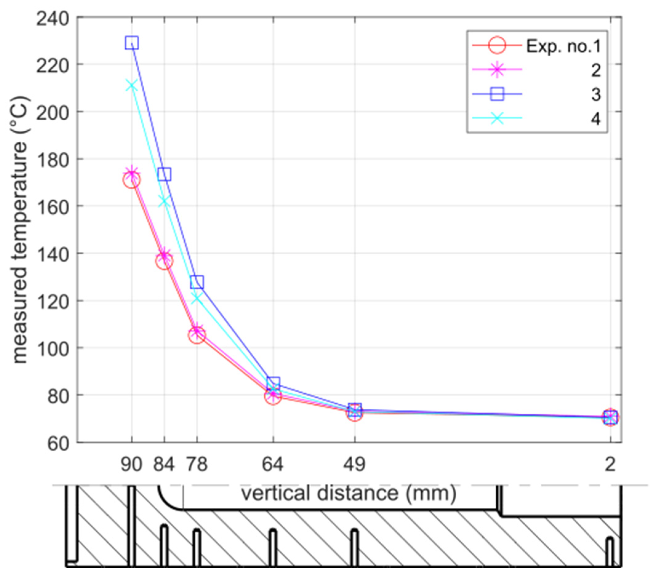
2.1. Temperature Measurements
- The experiment starts together with the temperature recordings.
- The water jet cooling is performed with a constant flow rate.
- The heating from the top part of the sample is initiated.
- The thermal steady state is achieved throughout the experiment.
- Temperature cooling curves are saved for the subsequent inverse calculation and post-processing of the heat dissipation rate (also referred to as the cooling power).
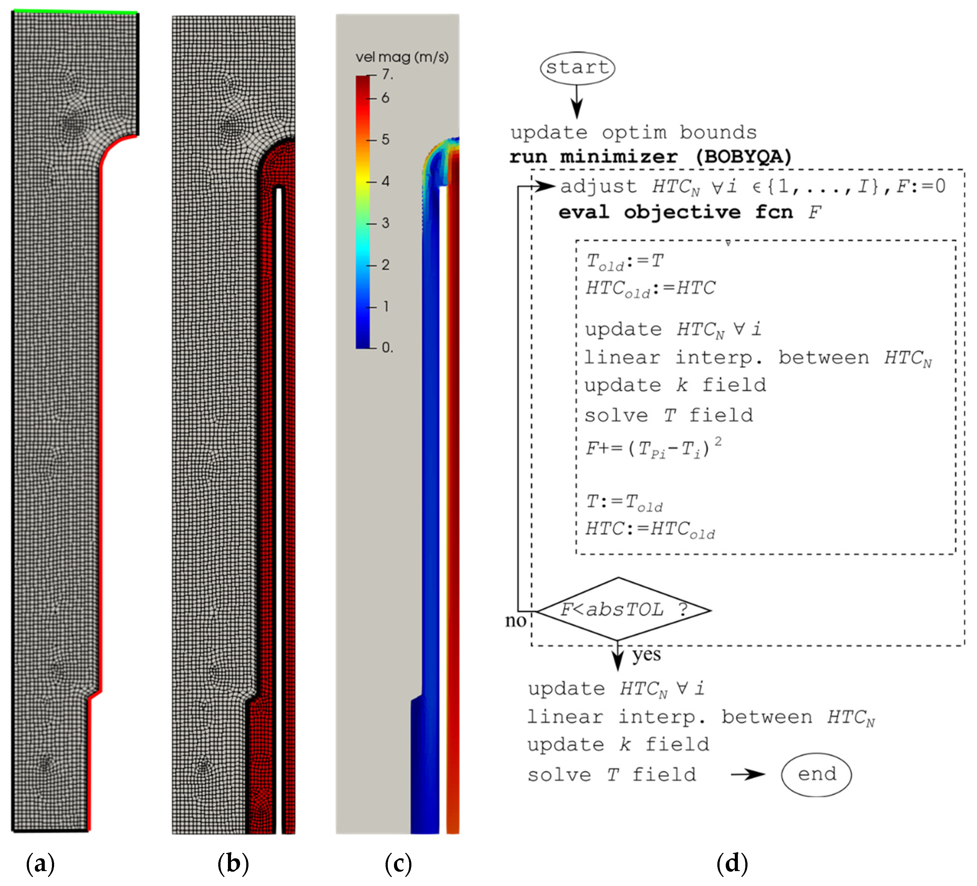
2.2. Inverse Heat Conduction Problem in 2D
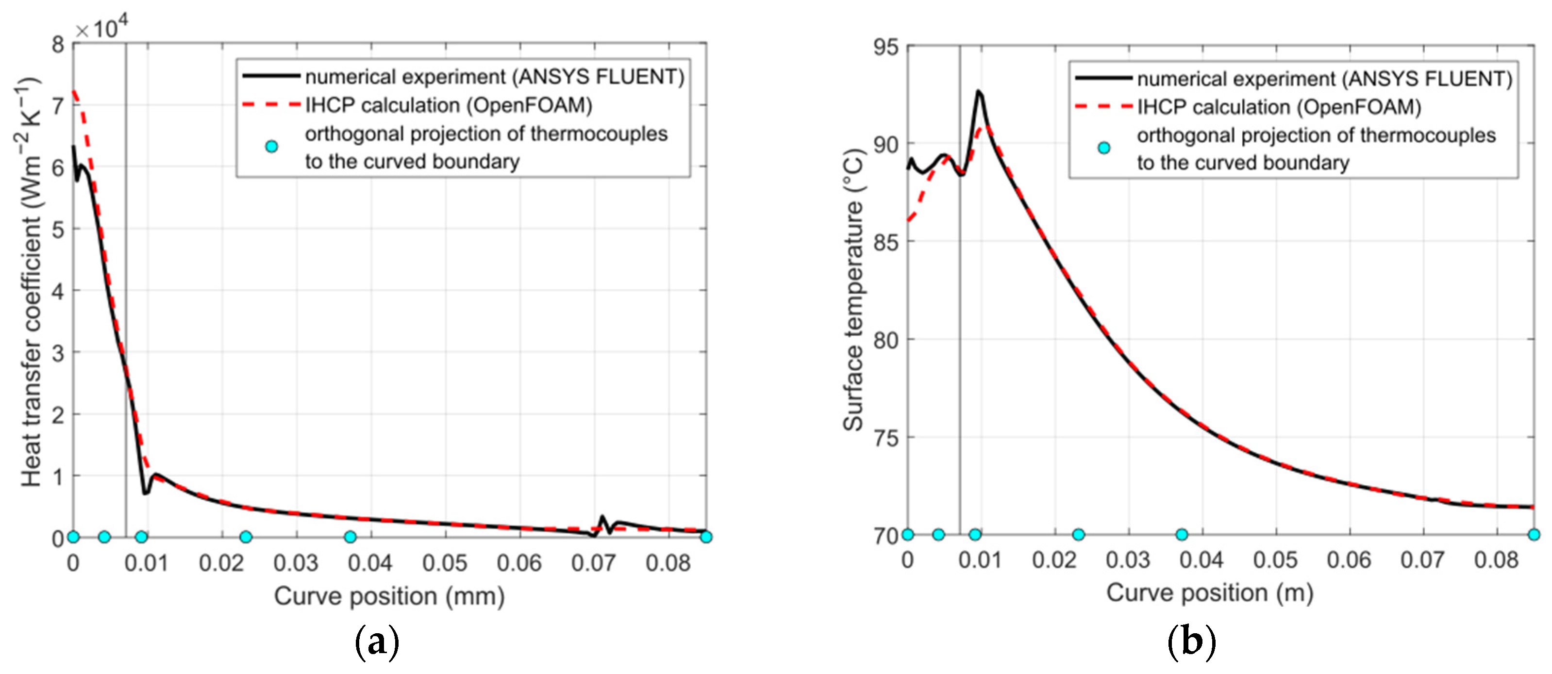
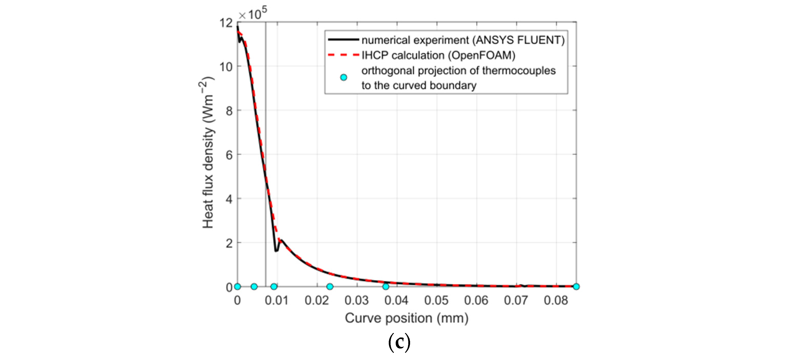
2.3. Verification of the IHCP Solver Using a Numerical Experiment
- There is no error regarding the temperature measurements (the exact values are defined at the exact locations);
- There is no error in defining the boundary conditions;
- There is no error in selecting the thermophysical properties;
- There is no error in specifying discretization and solution.
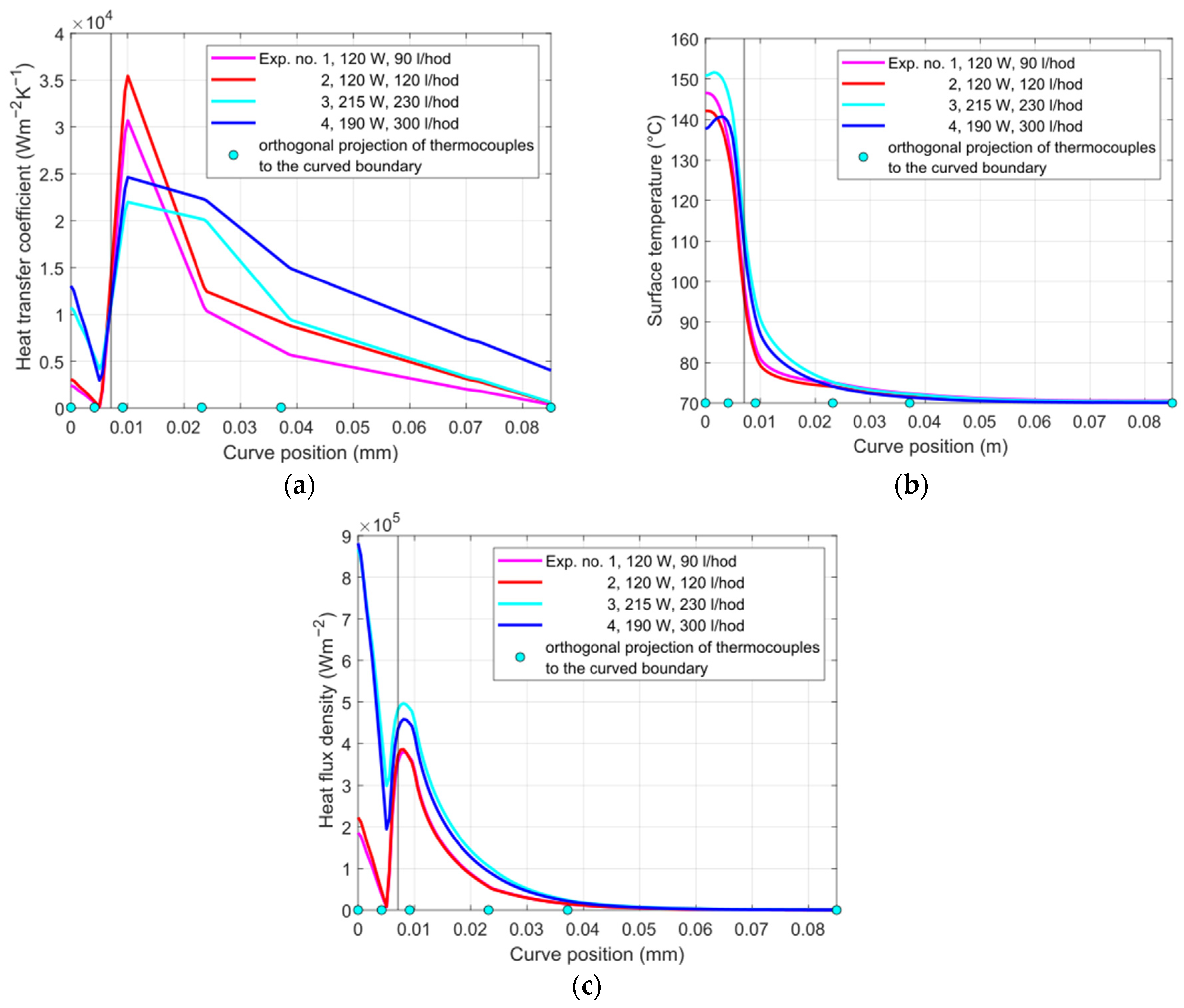
2.4. IHCP Calculations with Experimental Data
3. Results
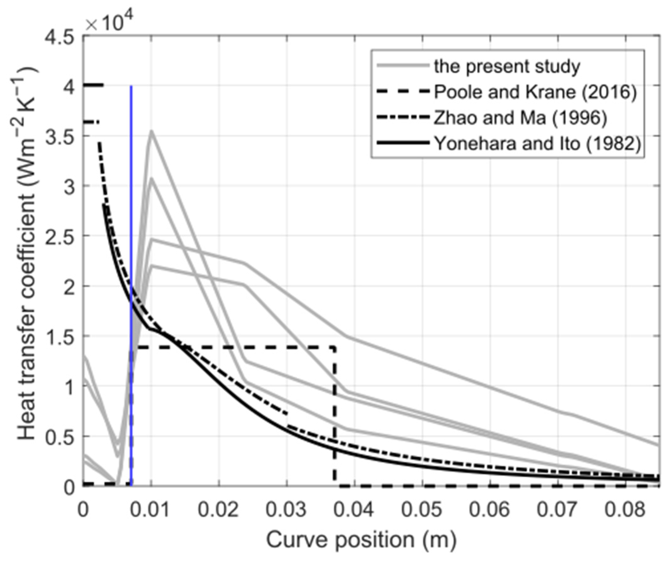
4. Discussion
5. Conclusions
Author Contributions
Funding
Data Availability Statement
Acknowledgments
Conflicts of Interest
Nomenclature
| F | objective or target function (K2) |
| HTC | heat transfer coefficient (Wm−2K−1) |
| k | thermal conductivity (Wm−1K−1) |
| q | heat flux (Wm−2) |
| T | temperature (K) |
| Ω | space domain (m) |
| Abbreviations | |
| BOBYQA | Bounded optimization by quadratic approximation |
| BC | Boundary condition |
| CFD | Computational fluid dynamics |
| Dievar | High-performance chromium–molybdenum–vanadium-alloyed hot work tool steel |
| HPDC | High-pressure die casting |
| NLopt | Nonlinear optimization toolbox |
| OpenFOAM | Open-source CFD package |
| RANS | Reynolds-averaged Navier–Stokes (equations) |
| PDE | Partial differential equation |
| PID | Proportional–integral–derivative controller |
| Subscripts | |
| i | summation index |
| I | number of thermocouples |
| N | a point on the curved boundary of the jet cooler generated by the orthogonal projection of the thermocouple tip, i.e., the point P |
| P | measuring point of thermocouple |
References
- Govender, G.; Möller, H.; Damm, O.F.R.A. Semisolid Processes. In Comprehensive Materials Processing; Elsevier: Amsterdam, The Netherlands, 2014; pp. 109–134. ISBN 978-0-08-096533-8. [Google Scholar]
- Kowalczyk, W.; Dańko, R.; Górny, M.; Kawalec, M.; Burbelko, A. Influence of High-Pressure Die Casting Parameters on the Cooling Rate and the Structure of EN-AC 46000 Alloy. Materials 2022, 15, 5702. [Google Scholar] [CrossRef]
- Murray, M.T.; Murray, M. High Pressure Die Casting of Aluminium and Its Alloys. In Fundamentals of Aluminium Metallurgy; Elsevier: Amsterdam, The Netherlands, 2011; pp. 217–261. ISBN 978-1-84569-654-2. [Google Scholar]
- Lumley, R.N. Progress on the Heat Treatment of High Pressure Die Castings. In Fundamentals of Aluminium Metallurgy; Elsevier: Amsterdam, The Netherlands, 2011; pp. 262–303. ISBN 978-1-84569-654-2. [Google Scholar]
- Jarfors, A.E.W.; Sevastopol, R.; Seshendra, K.; Zhang, Q.; Steggo, J.; Stolt, R. On the Use of Conformal Cooling in High-Pressure Die-Casting and Semisolid Casting. Technologies 2021, 9, 39. [Google Scholar] [CrossRef]
- Blondheim, D.J. System Understanding of High Pressure Die Casting Process and Data with Machine Learning Applications. Doctoral Thesis, Colorado State University, Fort Collins, CO, USA, 2021. [Google Scholar]
- Karkkainen, M.; Nastac, L. Numerical Modeling of Convective Heat Transfer for Turbulent Flow in “Bubbler” Cooling Channels. JOM 2019, 71, 772–778. [Google Scholar] [CrossRef]
- Gnielinski, V. Turbulent Heat Transfer in Annular Spaces—A New Comprehensive Correlation. Heat Transf. Eng. 2015, 36, 787–789. [Google Scholar] [CrossRef]
- Kawahara, H.; Nishimura, T. Transport Phenomenon in a Jet Type Mold Cooling Pipe. In Computational Methods and Experimental Measurements XIV; WIT Press: Algarve, Portugal, 2009; pp. 437–449. [Google Scholar]
- Sun, F.; Schwam, D.; Wang, G.-X.; Wallace, J.F. An Experimental Study on the Cooling Effect of Die Casting Die Insert Cooling Devices. In Proceedings of the Heat Transfer; ASMEDC: Washington, DC, USA, 2003; Volume 3, pp. 239–244. [Google Scholar]
- Fu, J. Uncertainty Quantification on Industrial High Pressure Die Casting Process. Master Thesis, Purdue University, West Lafayette, IN, USA, 2016. [Google Scholar]
- Taler, J.; Zima, W. Solution of Inverse Heat Conduction Problems Using Control Volume Approach. Int. J. Heat Mass Transf. 1999, 42, 1123–1140. [Google Scholar] [CrossRef]
- Fu, J.; Coleman, J.; Poole, G.; Krane, M.J.M.; Marconnet, A. Uncertainty Propagation Through a Simulation of Industrial High Pressure Die Casting. J. Heat Transf. 2019, 141, 112101. [Google Scholar] [CrossRef]
- Qiu, D.; Wang, C.; Luo, L.; Wang, S.; Zhao, Z.; Wang, Z. On Heat Transfer and Flow Characteristics of Jets Impinging onto a Concave Surface with Varying Jet Arrangements. J. Therm. Anal. Calorim. 2020, 141, 57–68. [Google Scholar] [CrossRef]
- Singh, A.; Chakravarthy, B.; Prasad, B. Numerical Simulations and Optimization of Impinging Jet Configuration. Int. J. Numer. Methods Heat Fluid Flow 2020, 31, 1–25. [Google Scholar] [CrossRef]
- Azimi, A.; Ashjaee, M.; Razi, P. Slot Jet Impingement Cooling of a Concave Surface in an Annulus. Exp. Therm. Fluid Sci. 2015, 68, 300–309. [Google Scholar] [CrossRef]
- Lyu, Y.; Zhang, J.; Liu, X.; Shan, Y. Experimental Study of Single-Row Chevron-Jet Impingement Heat Transfer on Concave Surfaces with Different Curvatures. Chin. J. Aeronaut. 2019, 32, 2275–2285. [Google Scholar] [CrossRef]
- Lyu, Y.; Zhang, J.; Wang, B.; Tan, X. Convective Heat Transfer on Flat and Concave Surfaces Subjected to an Impinging Jet Form Lobed Nozzle. Sci. China Technol. Sci. 2020, 63, 116–127. [Google Scholar] [CrossRef]
- Xie, Y.; Li, P.; Lan, J.; Zhang, D. Flow and Heat Transfer Characteristics of Single Jet Impinging on Dimpled Surface. J. Heat Transf. 2013, 135, 052201. [Google Scholar] [CrossRef]
- Singh, A.; Balaji, C. Heat Transfer Optimization Studies of Semi-Spherical Protrusions on a Concave Surface during Jet Impingement. Heat Transf. Eng. 2023, 1–24. [Google Scholar] [CrossRef]
- Ahmed, A.; Wright, E.; Abdel-Aziz, F.; Yan, Y. Numerical Investigation of Heat Transfer and Flow Characteristics of a Double-Wall Cooling Structure: Reverse Circular Jet Impingement. Appl. Therm. Eng. 2021, 189, 116720. [Google Scholar] [CrossRef]
- Pakhomov, M.A.; Terekhov, V.I. Numerical Study of Fluid Flow and Heat Transfer Characteristics in an Intermittent Turbulent Impinging Round Jet. Int. J. Therm. Sci. 2015, 87, 85–93. [Google Scholar] [CrossRef]
- Lee, D.H.; Chung, Y.S.; Won, S.Y. Technical Note the Effect of Concave Surface Curvature on Heat Transfer from a Fully Developed Round Impinging Jet. Int. J. Heat Mass Transf. 1999, 42, 2489–2497. [Google Scholar] [CrossRef]
- Joshi, J.; Sahu, S.K. Heat Transfer Characteristics of Flat and Concave Surfaces by Circular and Elliptical Jet Impingement. Exp. Heat Transf. 2022, 35, 938–963. [Google Scholar] [CrossRef]
- Hu, W.; Jia, Y.; Chen, X.; Le, Q.; Chen, L.; Chen, S. Determination of Secondary Cooling Zone Heat Transfer Coefficient with Different Alloy Types and Roughness in DC Casting by Inverse Heat Conduction Method. Crystals 2022, 12, 1571. [Google Scholar] [CrossRef]
- Bohacek, J.; Kominek, J.; Vakhrushev, A.; Karimi-Sibaki, E.; Lee, T. Sequential Inverse Heat Conduction Problem in OpenFOAM®. OpenFOAM J. 2021, 1, 27–46. [Google Scholar] [CrossRef]
- Weller, H.G.; Tabor, G.; Jasak, H.; Fureby, C. A Tensorial Approach to Computational Continuum Mechanics Using Object-Oriented Techniques. Comput. Phys. 1998, 12, 620. [Google Scholar] [CrossRef]
- Johnson, S. The NLopt Nonlinear-Optimization Package. Available online: http://ab-initio.mit.edu/nlopt (accessed on 24 February 2023).
- Powell, M.J.D. The BOBYQA Algorithm for Bound Constrained Optimization without Derivatives; Department of Applied Mathematics and Theoretical Physics: Cambridge, UK, 2009; p. 39. [Google Scholar]
- Leocadio, H. Interfaces and Heat Transfer in Jet Impingement on a High Temperature Surface. Ph.D. Thesis, Technische Universiteit Eindhoven, Eindhoven, The Netherlands, 2018. [Google Scholar]
- Webb, B.W.; Ma, C.-F. Single-Phase Liquid Jet Impingement Heat Transfer. In Advances in Heat Transfer; Elsevier: Amsterdam, The Netherlands, 1995; Volume 26, pp. 105–217. ISBN 978-0-12-020026-9. [Google Scholar]
- Ahmed, Z.U.; Sharif, M.A.R.; Nahian, N.A. Convective Heat Transfer from a Spherical Concave Surface Due to Swirling Impinging Jets Issuing from a Circular Pipe. Appl. Therm. Eng. 2024, 236, 121489. [Google Scholar] [CrossRef]
- Kura, T.; Fornalik-Wajs, E.; Wajs, J.; Kenjeres, S. Curved Surface Minijet Impingement Phenomena Analysed with ζ-f Turbulence Model. Energies 2021, 14, 1846. [Google Scholar] [CrossRef]
- Zuckerman, N.; Lior, N. Radial Slot Jet Impingement Flow and Heat Transfer on a Cylindrical Target. J. Thermophys. Heat Transf. 2007, 21, 548–561. [Google Scholar] [CrossRef]
- Garimella, S.V.; Rice, R.A. Confined and Submerged Liquid Jet Impingement Heat Transfer. J. Heat Transf. 1995, 117, 871–877. [Google Scholar] [CrossRef]
- Ma, C.F.; Zhao, Y.H.; Masuoka, T.; Gomi, T. Analytical Study on Impingement Heat Transfer with Single-Phase Free-Surface Circular Liquid Jets. J. Therm. Sci. 1996, 5, 271–277. [Google Scholar] [CrossRef]
- Ito, I.; Yonehara, N. Cooling Characteristics of the Impinging Water Jet on a Horizontal Plane: Part 1-Through a Single Nozzle. Trans. JSRAE 1982, 7, 99–106. [Google Scholar] [CrossRef]
- Arunkumar, K.; Bakshi, S.; Phanikumar, G.; Rao, T.V.L.N. Study of Flow and Heat Transfer in High Pressure Die Casting Cooling Channel. Met. Mater Trans. B 2023, 54, 1665–1674. [Google Scholar] [CrossRef]


| Exp. #1 | Exp. #2 | Exp. #3 | Exp. #4 | ||
|---|---|---|---|---|---|
| Flow rate | L/h | 90 | 120 | 230 | 300 |
| Inlet temperature | °C | 69.6 | 69.7 | 70.2 | 70.2 |
| Outlet temperature | °C | 70.8 | 70.5 | 71.0 | 70.7 |
| Cooling power | W | 120 | 120.0 | 213 | 190 |
| Copper temperature | °C | 600 | 600 | 550 | 550 |
| Steady-state readings | #1 | 173.8 | 171.1 | 229.0 | 211.2 |
| from thermocouples (°C): | #2 | 139.1 | 136.7 | 173.4 | 162.1 |
| #3 | 107.2 | 105.3 | 127.7 | 120.9 | |
| #4 | 80.6 | 79.5 | 84.8 | 82.6 | |
| #5 | 73.1 | 72.5 | 73.8 | 72.9 | |
| #6 | 70.9 | 70.5 | 70.5 | 70.1 |
| Parameter Name | Value |
|---|---|
| ddtScheme | steadyState |
| grad (T) | Gauss linear |
| Laplacian (k,T) | Gauss linear Corrected |
| interpolation | linear |
| snGradSchemes | orthogonal |
| under-relaxation | none |
| linear solver | PCG FDIC (tolerance 1 × 10⁻¹⁴) |
| nNonOrthogonalCorrectors | 1 |
| minimizer | BOBYQA (bounded quadratic) |
| maxTime (s) | 300 |
| initial HTC (Wm−2K−1) | 10,000 |
| lower bound of HTC (Wm−2K−1) | 0 |
| upper bound of HTC (Wm−2K−1) | 100,000 |
| Thermocouples: | #1 | #2 | #3 | #4 | #5 | #6 |
|---|---|---|---|---|---|---|
| Temperatures in | ||||||
| num. experiment (°C) | 190.447 | 143.354 | 113.892 | 87.237 | 77.483 | 71.516 |
| IHCP calculation (°C) | 190.447 | 143.353 | 113.891 | 87.237 | 77.483 | 71.516 |
| Exp. #1 | Exp. #2 | Exp. #3 | Exp. #4 | ||
|---|---|---|---|---|---|
| Goal function (K2) | 0.242 | 0.135 | 0.0109 | 1.22 × 10⁻⁷ | |
| #1 | −0.093 | −0.099 | −0.00034 | −0.000033 | |
| for thermocouples (K): | #2 | 0.202 | 0.215 | 0.00115 | 0.000062 |
| #3 | −0.144 | −0.146 | −0.00261 | −0.000128 | |
| #4 | −0.112 | 0.055 | 0.01609 | 0.000026 | |
| #5 | −0.247 | 0.115 | −0.05003 | 0.000007 | |
| #6 | 0.314 | 0.203 | 0.09037 | −0.000318 |
Disclaimer/Publisher’s Note: The statements, opinions and data contained in all publications are solely those of the individual author(s) and contributor(s) and not of MDPI and/or the editor(s). MDPI and/or the editor(s) disclaim responsibility for any injury to people or property resulting from any ideas, methods, instructions or products referred to in the content. |
© 2023 by the authors. Licensee MDPI, Basel, Switzerland. This article is an open access article distributed under the terms and conditions of the Creative Commons Attribution (CC BY) license (https://creativecommons.org/licenses/by/4.0/).
Share and Cite
Bohacek, J.; Mraz, K.; Krutis, V.; Kana, V.; Vakhrushev, A.; Karimi-Sibaki, E.; Kharicha, A. Experimental and Numerical Investigations into Heat Transfer Using a Jet Cooler in High-Pressure Die Casting. J. Manuf. Mater. Process. 2023, 7, 212. https://doi.org/10.3390/jmmp7060212
Bohacek J, Mraz K, Krutis V, Kana V, Vakhrushev A, Karimi-Sibaki E, Kharicha A. Experimental and Numerical Investigations into Heat Transfer Using a Jet Cooler in High-Pressure Die Casting. Journal of Manufacturing and Materials Processing. 2023; 7(6):212. https://doi.org/10.3390/jmmp7060212
Chicago/Turabian StyleBohacek, Jan, Krystof Mraz, Vladimir Krutis, Vaclav Kana, Alexander Vakhrushev, Ebrahim Karimi-Sibaki, and Abdellah Kharicha. 2023. "Experimental and Numerical Investigations into Heat Transfer Using a Jet Cooler in High-Pressure Die Casting" Journal of Manufacturing and Materials Processing 7, no. 6: 212. https://doi.org/10.3390/jmmp7060212
APA StyleBohacek, J., Mraz, K., Krutis, V., Kana, V., Vakhrushev, A., Karimi-Sibaki, E., & Kharicha, A. (2023). Experimental and Numerical Investigations into Heat Transfer Using a Jet Cooler in High-Pressure Die Casting. Journal of Manufacturing and Materials Processing, 7(6), 212. https://doi.org/10.3390/jmmp7060212