Article

Modeling of Surface Roughness in Honing Processes by Using Fuzzy Artificial Neural Networks

by
Irene Buj-Corral
1,*,
Piotr Sender
1,2 and
Carmelo J. Luis-Pérez
3,*
1
Department of Mechanical Engineering, Barcelona School of Industrial Engineering (ETSEIB), Universitat Politècnica de Catalunya-Barcelona Tech (UPC), 08028 Barcelona, Spain
2
Institute of Manufacturing and Materials Technology, Faculty of Mechanical Engineering and Ship Technology, Gdańsk University of Technology, ul. Narutowicza 11/12, 80-233 Gdańsk, Poland
3
Engineering Department, Public University of Navarre (UPNA), Arrosadia Campus, 31006 Pamplona, Spain
*
Authors to whom correspondence should be addressed.
J. Manuf. Mater. Process. 2023, 7(1), 23; https://doi.org/10.3390/jmmp7010023
Submission received: 25 November 2022 / Revised: 23 December 2022 / Accepted: 31 December 2022 / Published: 15 January 2023
(This article belongs to the Special Issue Advances in Precision Machining Processes)

Abstract

:
Honing processes are abrasive machining processes which are commonly employed to improve the surface of manufactured parts such as hydraulic or combustion engine cylinders. These processes can be employed to obtain a cross-hatched pattern on the internal surfaces of cylinders. In this present study, fuzzy artificial neural networks are employed for modeling surface roughness parameters obtained in finishing honing operations. As a general trend, main factors influencing roughness parameters are grain size and pressure. Mean spacing between profile peaks at the mean line parameter, on the contrary, depends mainly on tangential and linear velocity. Grain Size of 30 and pressure of 600 N/cm2 lead to the highest values of core roughness (Rk) and reduced valley depth (Rvk), which were 1.741 µm and 0.884 µm, respectively. On the other hand, the maximum peak-to-valley roughness parameter (Rz) so obtained was 4.44 µm, which is close to the maximum value of 4.47 µm. On the other hand, values of the grain size equal to 14 and density equal to 20, along with pressure 600 N/cm2 and both tangential and linear speed of 20 m/min and 40 m/min, respectively, lead to the minimum values of core roughness, reduced peak height (Rpk), reduced valley depth and maximum peak-to-valley height of the profile within a sampling length, which were, respectively, 0.141 µm, 0.065 µm, 0.142 µm, and 0.584 µm.

1. Introduction

The surface texture of the cylinder liners influences greatly the performance of combustion engines, especially regarding friction, oil consumption, emissions, wear, etc. [1]. It also affects the ring-pack performance [2]. Specifically, the honing angle has a great impact on the friction coefficient in the liner-ring pair. In general, low coefficient of friction is obtained when a low honing angle is employed, for example 40° [3].
In order to analyze and compare different surface topographies, several roughness parameters have previously been used in honing processes. In [4], Buj et al. employed regression models to predict roughness, material removal rate and tool wear in the rough, semi-finish and finish operations. They found that roughness is mainly influenced by grain size and density of abrasive. A sensitivity analysis was presented in their study for a multi-objective optimization process. In Kanthababu et al. [5] the surface topography was characterized by average roughness (Ra) and all five bearing area parameters ((Rpk), (Rk), (Rvk), (Mr1) and (Mr2)). These authors found that Ra can be replaced effectively by Rk in finishing honing operations to control the final surface topography. Barros et al. [6] studied the influence of grain size and of the number of strokes on the bearing area parameters in flexible honing. They observed that grain size influenced mainly parameters (Rk), (Rpk), (Mr2), and (Rp/Rt), while the number of strokes influenced (Rpk). Sadizade et al. [7] studied the (Rk) family parameters in plateau honing operations of Diesel engines. They define a two-stage process (instead of the usual three-stage process) containing rough honing (with the consecutive application of high and low pressure) and plateau honing, in which total honing time is thus reduced. (Rpk) parameter depends mainly on low pressure, low time and plateau pressure. (Rk) depends on low pressure, plateau pressure and the plateau stroke number. (Rvk) depends on low pressure and low time. Thus, low pressure is an important variable affecting the three a.m. parameters. Ma et al. [8] studied the plateau honing operation of CuNiCr iron liners [8] and observed that a honing angle of 58° implies better tribological properties for the liners. In addition, they observed that the tribological properties are more related to parameters Rk and Rpk than to parameter Ra.
High correlations between roughness parameters are found in honing processes. Deepak Lawrence et al. [9] predicted the bearing area parameters from images of the honed surfaces. They found high correlation between the Rk family parameters determined with an image instrument and the same parameters measured with a stylus instrument. Highest correlation values of 0.81 and 0.82 were reported for Rpk and Spk parameters, respectively, which are related to the profile peaks. Pawlus et al. [10] studied the plateau-honing process and found correlations between the (Rk) family parameters and the (Rq) family parameters. They found that (Rmr1) and (Rmr2) are strongly correlated with (Rmq), and that the peak parameters (and the valley parameters) of the two families are also correlated.
Other roughness parameters that are related to the shape of the profile, such as kurtosis (Rku) or skewness (Rsk) are useful in one-stage processes such as honing [11]. For example, they allow monitoring wear of the cylinder surface [12]. Both parameters are known to be correlated and, for this reason, they are not recommended in two-stage processes like plateau-honing [13]. In Gaussian ordinate distributions, (Rsk) is usually close to 0, while (Rku) is similar to 3 [13]. Areal (Sku) and (Ssk) parameters were determined in semi-finishing honing processes by Buj-Corral et al. [14]. They found (Ssk) values similar to 0 and (Sku) values above 3 in all cases.
Spacing roughness parameters such as the mean width of roughness profile (RSm) have been reported to decrease in superfinishing operations [15]. In general, parameter (RSm) depends on the size of the scratches produced by the grains in abrasive machining processes, for example in belt finishing [16]. In plateau honing processes, Pawlus et al. [17] observed that, after applying a Gaussian filter to the roughness signal, the (RSm) parameter decreased.
Design of experiments (DOE) combined with artificial neural networks (ANN) have been widely used over the last few years to analyze the behavior of different output variables. In the literature, several studies can be found that deal with the application of soft computing for the modelling of different manufacturing processes. For example, the research study by Lalwani et al. [18] compared response surface methodology (RSM) and ANN for modeling the wire electrical discharge machining (WEDM) process. Among their results, these authors found that ANN had higher accuracy than RSM. Likewise, in Mirifar et al. [19] a feedforward neural network and Bayesian backpropagation algorithm were used to predict forces and roughness in grinding processes by using an acoustic emission sensor. These authors found, among their results, that ANNs were able to model obtained roughness with high precision. As for honing processes, Buj et al. [20] obtained an adaptive indirect ANN model in which the values of the process parameters are predicted from the measured Rk, Rpk and Rvk values.
On the other hand, fuzzy artificial neural networks (ANFIS) have also been employed to model machining processes. In a study from Aamir et al. [21] Taguchi design of experiments and fuzzy logic were employed to predict surface roughness and hole size in multi-hole drilling. Furthermore, in the work by Alajmi et al. [22], surface roughness obtained in dry and cryogenic turning of AISI 304 stainless steel was modeled using ANFIS-QPSO (fuzzy artificial neural networks with quantum particle swarm optimization). These authors found that ANFIS-QPSO was an effective and highly accurate method. Shivakoti et al. [23] analyzed the influence of feed, speed, and depth of cut on material removal rate, surface roughness and cutting force, in turning EN31 alloy steel by using ANFIS models. These authors found that ANFIS had high accuracy in predicting the output variables analyzed in their study. Regarding abrasive machining processes, Nguyen et al. [24] used the ANFIS-GPR (fuzzy artificial neural networks with gaussian process regression) hybrid algorithm with Taguchi analysis to model surface roughness in grinding operations. The ANFIS-GPR algorithm provided better predictability than ANFIS and Taguchi.
In this work, ANFIS models are applied to roughness parameters in finishing honing processes. It will help to select appropriate process parameters to improve obtained roughness within the current range of variation and parameters considered. Different roughness parameters are considered, including the (Rk) family parameters, kurtosis (Rku), skewness (Rsk) and the mean width of the roughness profile (RSm), which has been scarcely studied in the literature about honing processes. In addition, the application of ANFIS models to honing processes allows obtaining models with high fit values for the different roughness parameters.
The remaining sections of this present study are structured as follows: Section 2 corresponds to materials and methods; Section 3 contains the results and discussion; and in Section 4 the main conclusions of the work are presented.

2. Materials and Methods

In this section the methodology and the experiments carried out for modeling the honing process are outlined.

2.1. Research Methodology

To obtain the relationship between the response variables and the input variables, a set of experiments was carried out. These experiments were defined according to a two- level fractional factorial design 25−1 with three center points, as shown in Table 1. The levels of variation in the input variables were selected considering the experience of the authors in similar processes. The input variables considered in this study were particle size, density, pressure, and both tangential and linear velocity, since these are the parameters that most influence the response variables to be analyzed.
The output variables (response variables) analyzed in this study were: Core Roughness (Rk (µm)), Reduced peak height (Rpk (µm)), Reduced valley depth (Rvk (µm)), Material ratio (Mr1 (%) and Mr2 (%)), Maximum peak-to-valley height of the profile within a sampling length (Rz (µm)), Skewness (Rsk), Kurtosis (Rku) and Mean spacing between profile peaks at the mean line (RSm (µm)). That is, all five bearing area parameters (Rpk, Rk, Rvk, Mr1 and Mr2) were considered and, additionally, Rz, Rsk, Rku and RSm were analyzed in this present study as output variables.
As mentioned in the Section 1, in Kanthababu et al. [5] it was found that Ra can effectively be replaced by (Rk) in finishing honing operations to control the final surface topography. All bearing parameters, and (Rsk), (Rku) and (RSm) were also considered because these are the most useful parameters to analyze the honed parts. Therefore, these are the parameters whose influence is to be analyzed in this study.
As mentioned in the Section 1, it was found in M. Kanthababu et al. [5] that Ra can be effectively replaced by (Rk) in finish honing operations to control the final surface topography, and all bearing parameters and (Rsk), (Rku) and (RSm) were also taken into account because these are the most useful parameters to analyze honed parts. Therefore, these are the parameters whose influence will be analyzed in this study
Regarding the set-up of the experiments required to carry out the honing process, a horizontal test honing machine was employed from Honingtec S.A. Steel St-52 cylinders of internal diameter 50 mm and length 150 mm were employed, as Figure 1 shows.
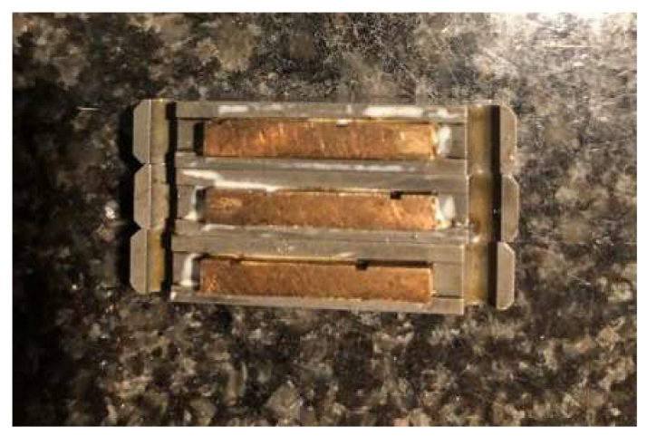
In this present study cBN honing stones with metallic bond were used, as can be observed in Figure 2.
Once the experiments were planned, the different honed conditions were employed to different cylinders, and then the surface roughness were measured on the manufactured parts, as explained in Section 2.2. From these results, a FIS was developed and then the parameters of the FIS’s membership functions were tuned by using an ANFIS. Then the obtained results were discussed and comparted with those reported by other researchers found in the specialized bibliography dealing with honing.

2.2. Surface Roughness Measurements

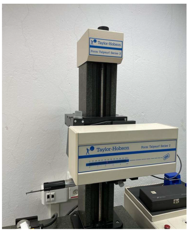
Roughness was measured with a Taylor Hobson Talysurf 2 contact roughness meter, as shown in Figure 3, with a Gaussian filter with cut-off value of 0.8 mm. Evaluation length was 4 mm. A diamond tip was used with tip radius of 2 µm and tip angle of 90°. Resolution of the inductive sensor was 18 nm and the measuring force was 1 mN.
Measurement results obtained in the honing test are presented in Table 2. The results for average roughness (Ra) are not included in this study and will be presented elsewhere.
The results shown in Table 2 were employed to develop the FIS and then optimized by an ANFIS as shown in the next section.

2.3. FIS Modeling

Figure 4 shows the membership functions for fuzzification of the five different inputs, which are based on a Gaussian function as Equation (1) shows:
μ = e x c 2 2 σ 2
To develop the FIS, the first sixteen results of the honing experiments shown in Table 2 were used. Figure 4 shows the membership functions for fuzzification of the inputs. These functions can be obtained after substituting the values shown in Table 3, in Equation (1), for each of the input variables considered in the present study, respectively. The membership functions’ values are show in Table 3. These values were selected from the procedure explained in [27]. In this study the Gaussian membership functions were implemented by using the Fuzzy Logic Toolbox™ of MatlabTM2020a [24].
The aggregation method employed is the sum of fuzzy sets. In this present case, the aggregated output is obtained from the weighted average of all output rules. Both the implication method and the output of the Sugeno FIS are shown in Equations (2) and (3) [27,28,29]:
w j x = A n d M e t h o d μ 1 x 1 , , μ n x n
o u t p u t j = j = 1 N u m b e r   o f   r u l e s w j z j j = 1 N u m b e r   o f   r u l e s w j
As previously mentioned, zero-order Sugeno FISs were developed for each of the output variables, where output corresponds to Rk, Rpk, Rvk, Mr1, Mr2, Rz, Rsk, Rku and RSm. Each of the FISs have a set of n rules of the form shown by Equation (4), where x i (i = 1,2,...5) corresponds to the independent variable, and z j corresponds to the output obtained in each experiment and two membership functions are selected for each of the independent variables (k = 1, 2), as previously mentioned.
i f   x 1   i s   x 1 k   a n d   x 2   i s   x 2 k   a n d a n d   x 5   i s   x 5 k   t h e n   o u t p u t j   i s   z j
Table 4 shows the rules that have been employed in this present study which have been developed from Equation (3) and from the experimental data shown in Table 3.
As previously mentioned, once the Sugeno FIS were developed an ANFIS was used to adjust the membership functions’ parameters by using the Fuzzy Logic Toolbox™ of MatlabTM2020a [28]. As an example, Figure 5 shows the output of the ANFIS for experiment number 10 in the case of Mr2. In order to optimize the values of the membership functions, the optimization type was “tuning” and the method “anfis”. To obtain these tuned FIS, all the experimental data were employed. Detailed information about the algorithm employed by the ANFIS can be found in the research study of Jang [30].

3. Discussion and Results

As can be seen in Table 2, as a general trend, lower (Rk), (Rpk), (Rvk) and (Rz) values were obtained in the first 8 experiments, corresponding to low grain size, than in experiments 9 to 16, corresponding to high grain size. In plateau-honing experiments with diamond stones, Lawrence et al. [9] reported higher (Rk) values up to 2.25 µm and higher (Rvk) values up to 2.06 µm. They also obtained lower (Rpk) values up to 0.55 µm, probably because the plateau operation smoothened the previous peaks.
As for skewness (Rsk), which measures the symmetry of the profile, mainly negative values were obtained, corresponding to profiles with higher valley depths than peak heights. Experiments 9 to 16, obtained with high grain size of 30, provided (Rsk) values that are closer to zero and, in some cases, slightly positive up to 0.237 for experiment 9. All the experiments carried out with low grain size of 15 (experiments 1 to 8) showed negative (Rsk) values, with a low value of -2.217 for experiment 5. As a general trend, a honed surface will show (Rsk) values that are negative or slightly positive (between −1.5 and 0.5 approx.) [31], while a plateau-honed surface will have negative skewness [31,32]. A negative (Rsk) value favors the retention of fluids by a certain surface [33].
Regarding kurtosis (Rku), which evaluates the peakedness of the roughness profile, higher values were obtained for the experiments with grain size 15 (up to more than 18 for experiment 3) than for grain size 30 (below 7 in all cases). High kurtosis is related to sharp peaks. For instance, in honing processes, Kang et al. [12] reported (Sku) values of around 3.2 for an unworn surface, which increased with the running-in operation up to more than 10. As a general trend, honing processes provide (Rku) ranging from approx. 3 to more than 10 [31], while in plateau-honing (Rku) will be higher than 3 [31,32].
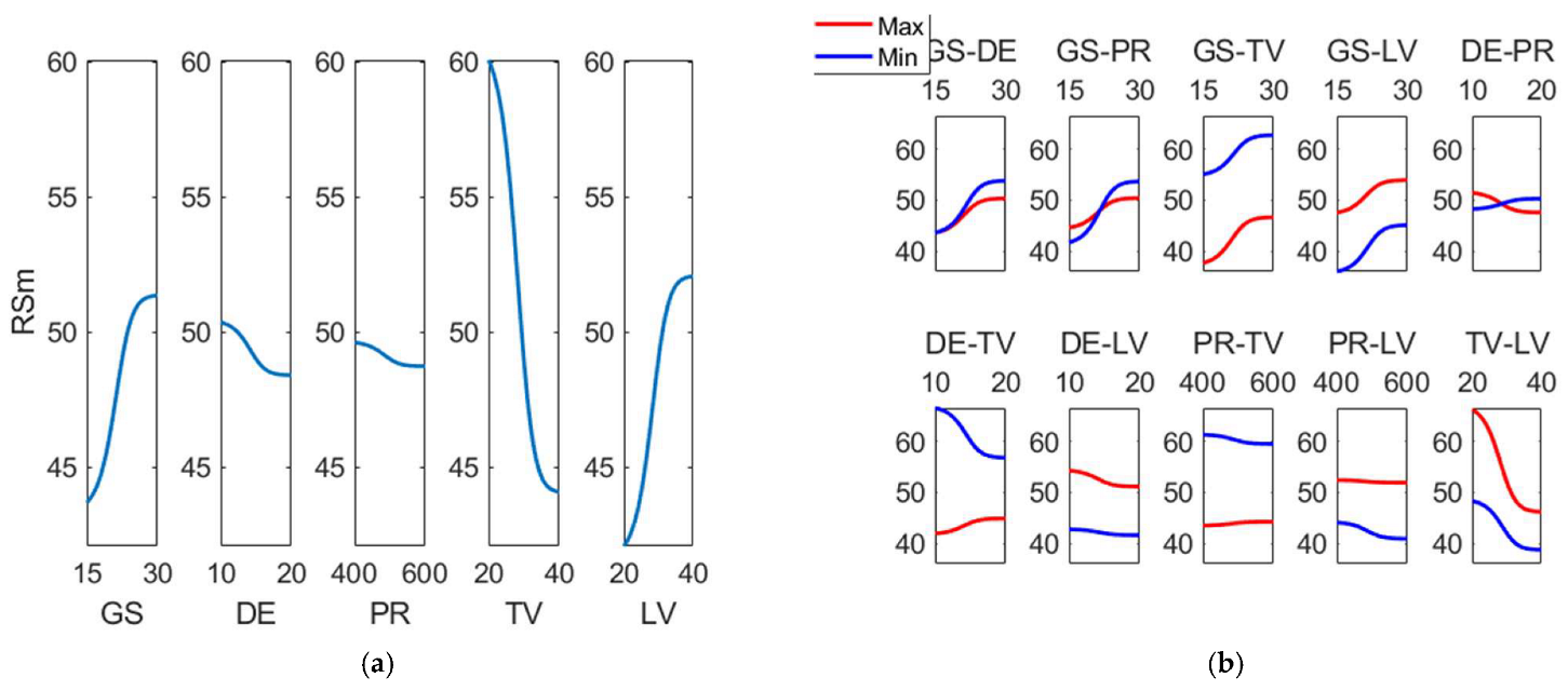
As for (Rsm), as a general trend higher values were reported in this work for grain size 30 (up to 75 μm) than for grain size 15 (up to 59 μm). The (Rsm) values obtained are similar to those of 62.3 µm reported by Grzesik et al. in turning + superfinishing operations [15]. In periodic roughness profiles, for example those obtained in turning and milling operations, (Rsm) is related to feed [34]. However, in more irregular profiles such as those obtained in abrasive machining processes, (Rsm) is related to grain size and depth of the grain [35].
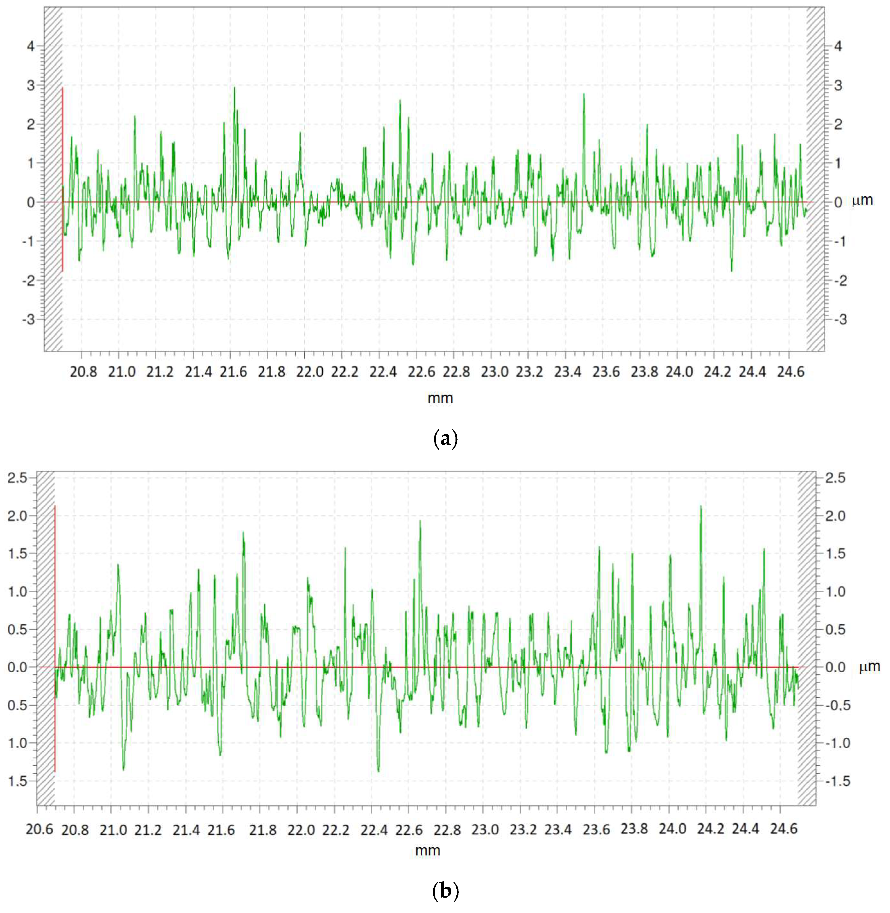
Figure 6 provides two different roughness profiles corresponding to experiments 9 and 11. They were both obtained with high grain size of 30 and high density of 20. However, experiment 9 was conducted at high pressure of 600 N/mm2, while experiment 11 was conducted at low pressure of 400 N/mm2.
Higher peaks (up to 3 µm high) and lower valleys (up to 1.8 µm deep) are obtained with high pressure (Figure 6a) than with low pressure (Figure 6b). This suggests that higher pressure leads to deeper scratch marks on the workpiece’s surface [36]. On the other hand, in rough honing processes pressure is known to affect not only roughness but also the cylindricity error of the parts [37].
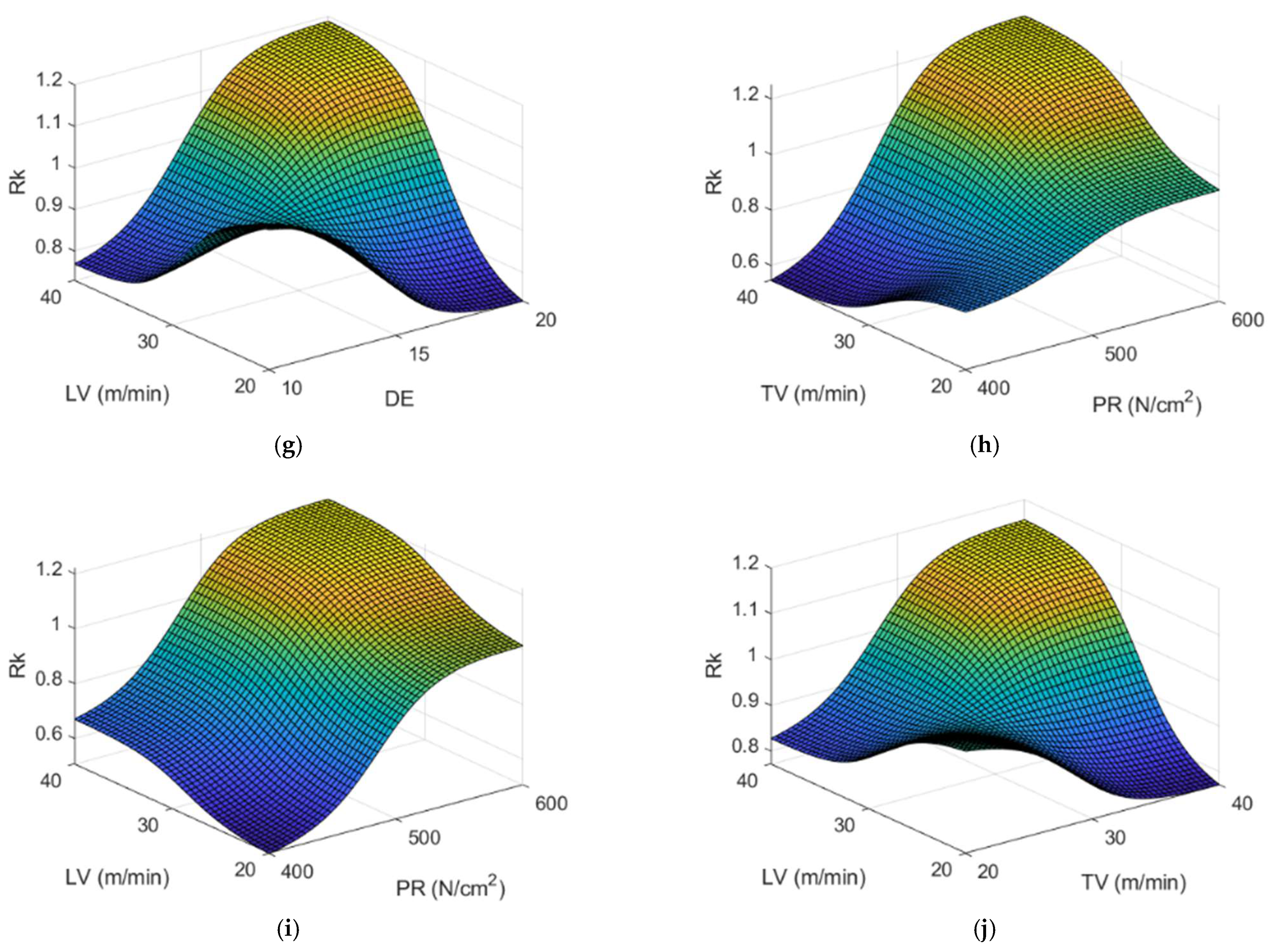
From the experimental values obtained after the design of experiments deployed in Table 2, a fuzzy inference system was developed for each of the response variables. Once these FISs were obtained, ANFISs were employed to adjust the values of the membership functions in order to obtain greater precision in the models thus obtained. The results obtained are shown below. As can be observed, Figure 7 shows the response surface plots for (Rk), for different pairs of variables, which have been obtained by using the ANFIS, where two independent variables are varied within their variation levels while the rest are kept at their central values.
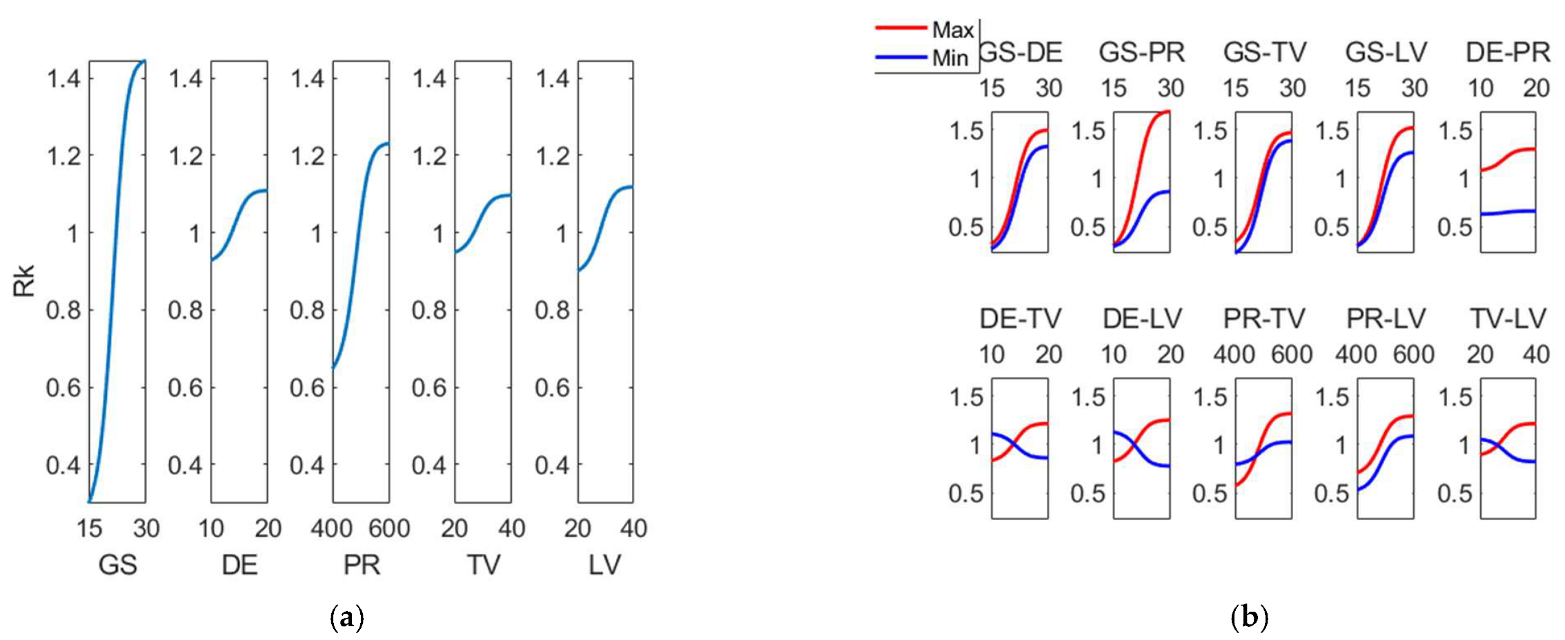
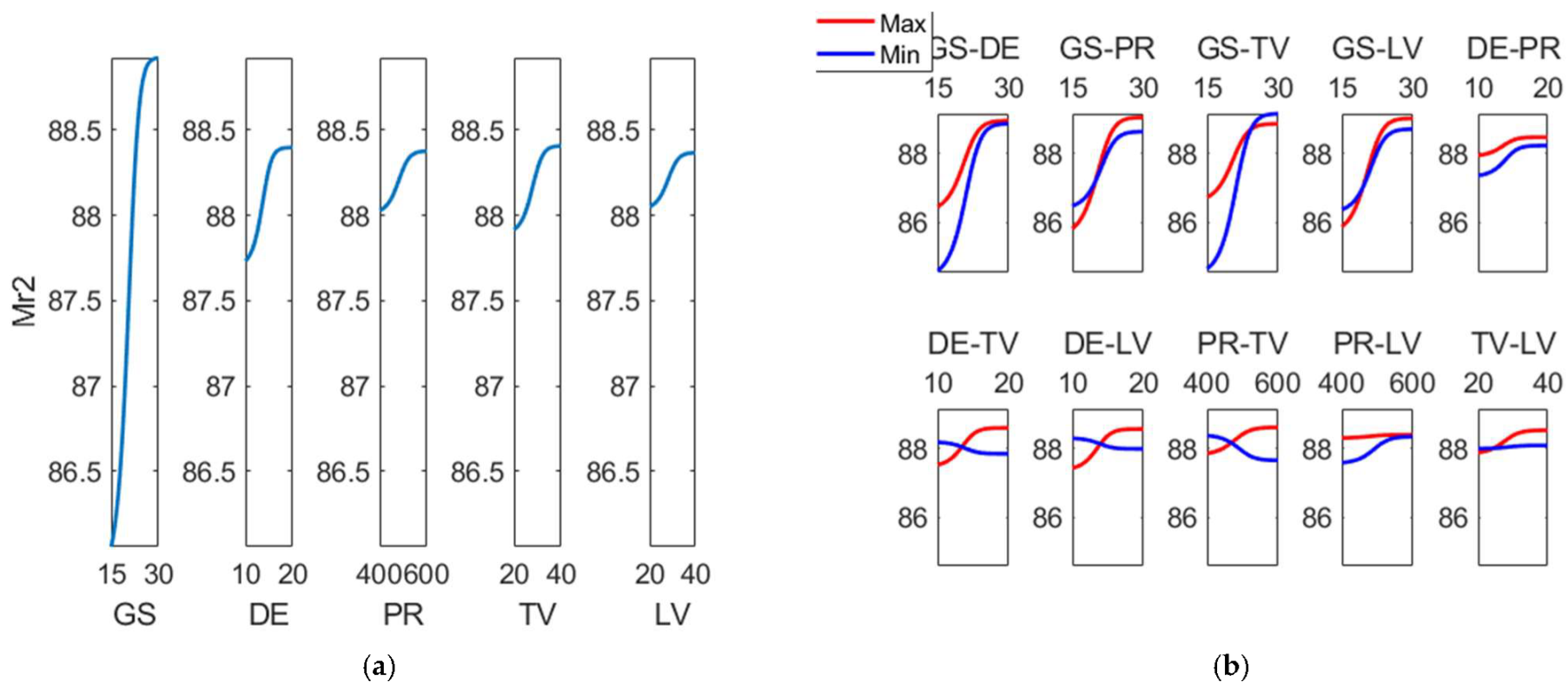
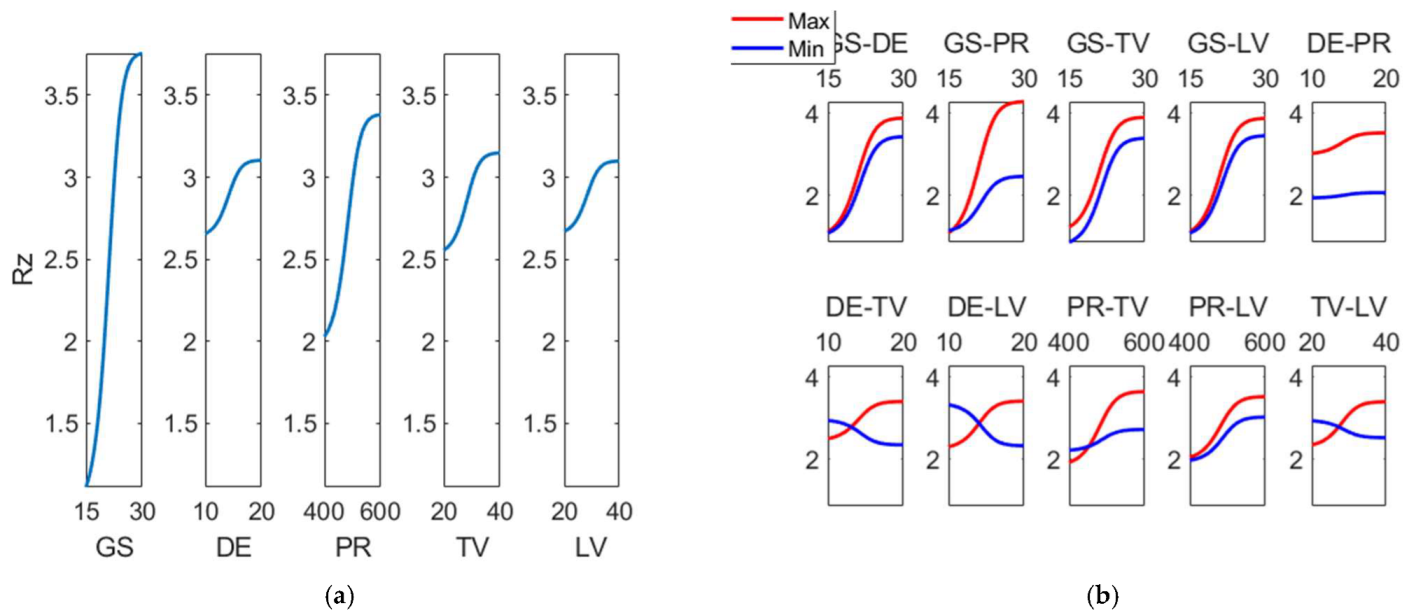
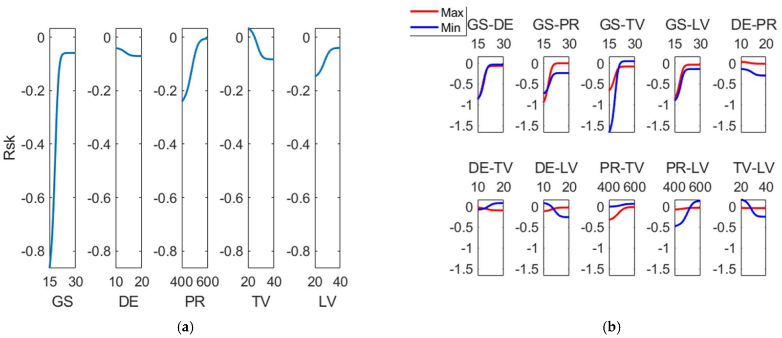
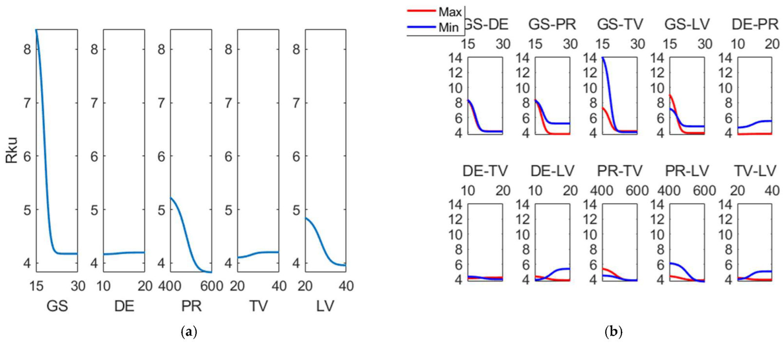
Similarly, Figure 8 depicts the main effects plot and the interaction plots for (Rk). The main effects plot is obtained from the variation in a variable between its lower and upper limits, while the remaining ones are kept at their central values and the interaction effects plot is obtained for each pair of variables, while the others are kept at their central values. This procedure is followed for all roughness parameters considered in the present study.
In Figure 8 it can be observed that the main factor influencing (Rk) parameter is grain size (GS), followed by pressure (PR). As for the interactions, most significant ones are related to parameter GS, for example, GS-DE, GS-PR, GS-TV and GS-LV. Caetano Barros et al. observed that (Rk) in honing processes is greatly dependent on grain size [6]. They used mesh sizes of 400 and 800, respectively. For example, mesh size of 400 in the Norton scale corresponds to particle size of around 46 µm (semifinishing honing).
Likewise, Figure 9 contains the main effects plot as well as the interaction effects plot for reduced peak height (Rpk). As can be observed, the main factors affecting roughness are grain size (GS) and pressure (PR), while main interactions are GS-DE, GS-PR, GS-TV and GS-LV. This behavior is similar to that of the (Rk) parameter. These results are in accordance with those of Caetano Barros et al. [6], who found a great influence of grain size on (Rpk) parameter. On the other hand, Figure 10 depicts the main effects plot and the interaction effects plot for (Rvk). Main effects for reduced peak height (Rvk) are grain size and pressure, and the most significant interactions are GS-DE, GS-PR, GS-TV and GS-LV. On the contrary, Caetano Barros et al. reported that (Rv) parameter remained almost unchanged when grain size was varied [6].
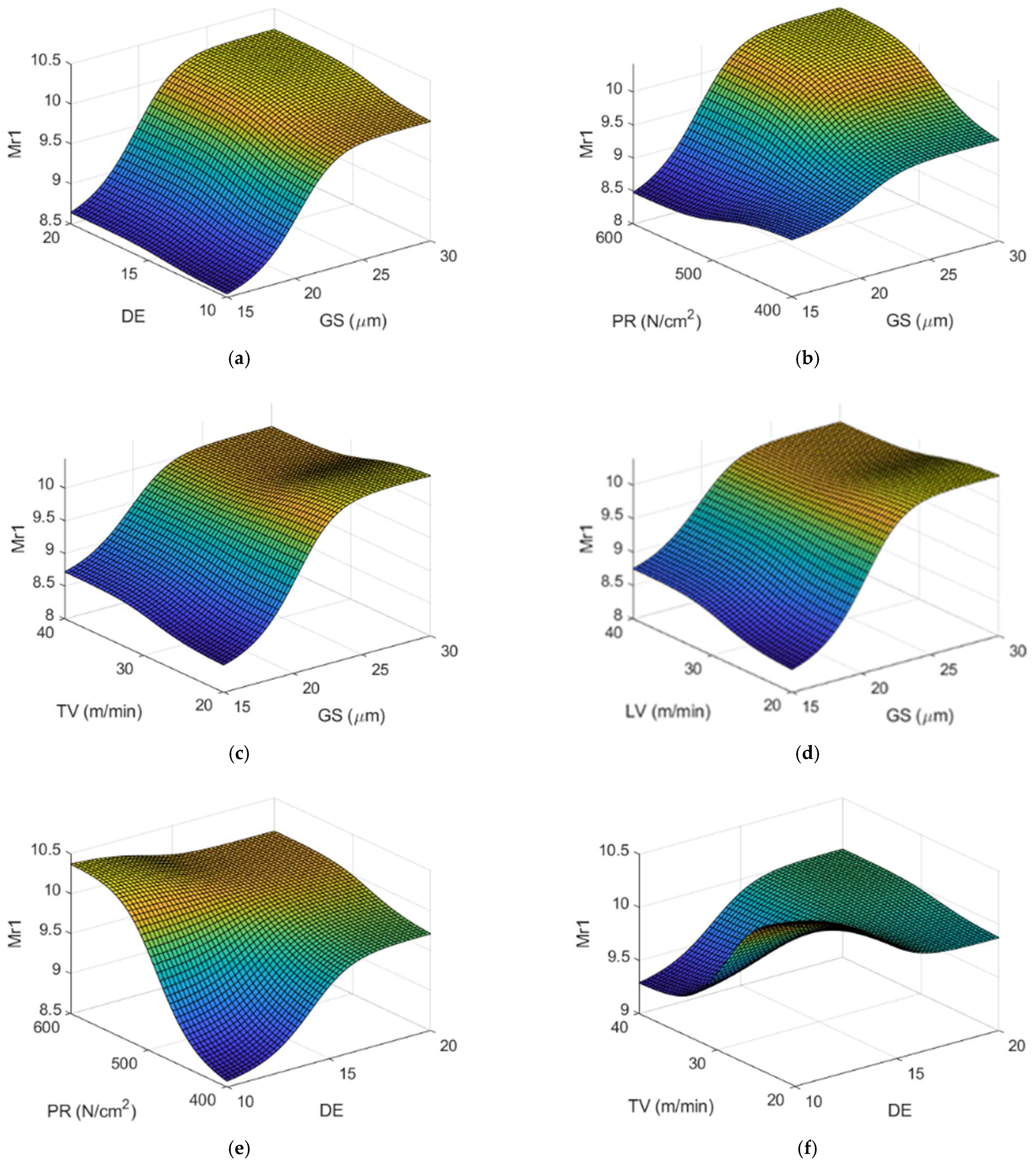
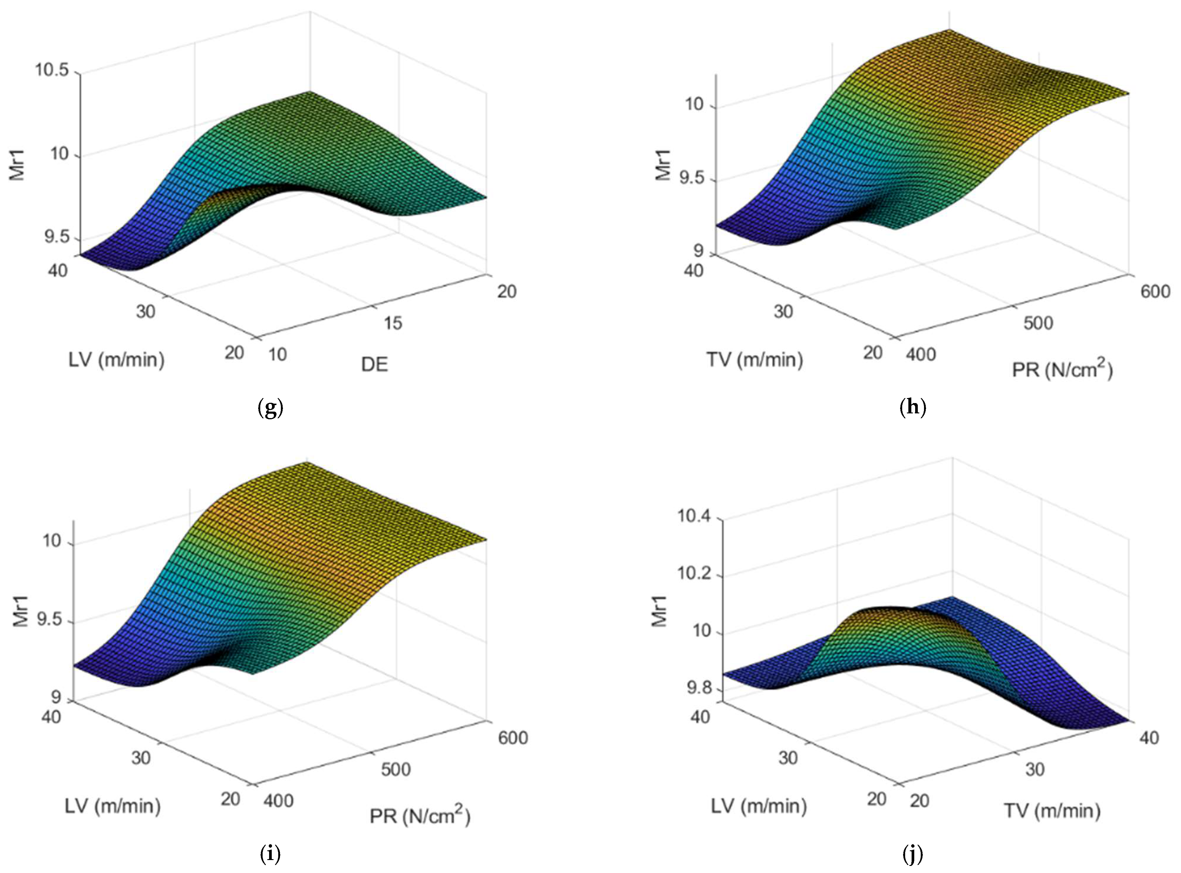
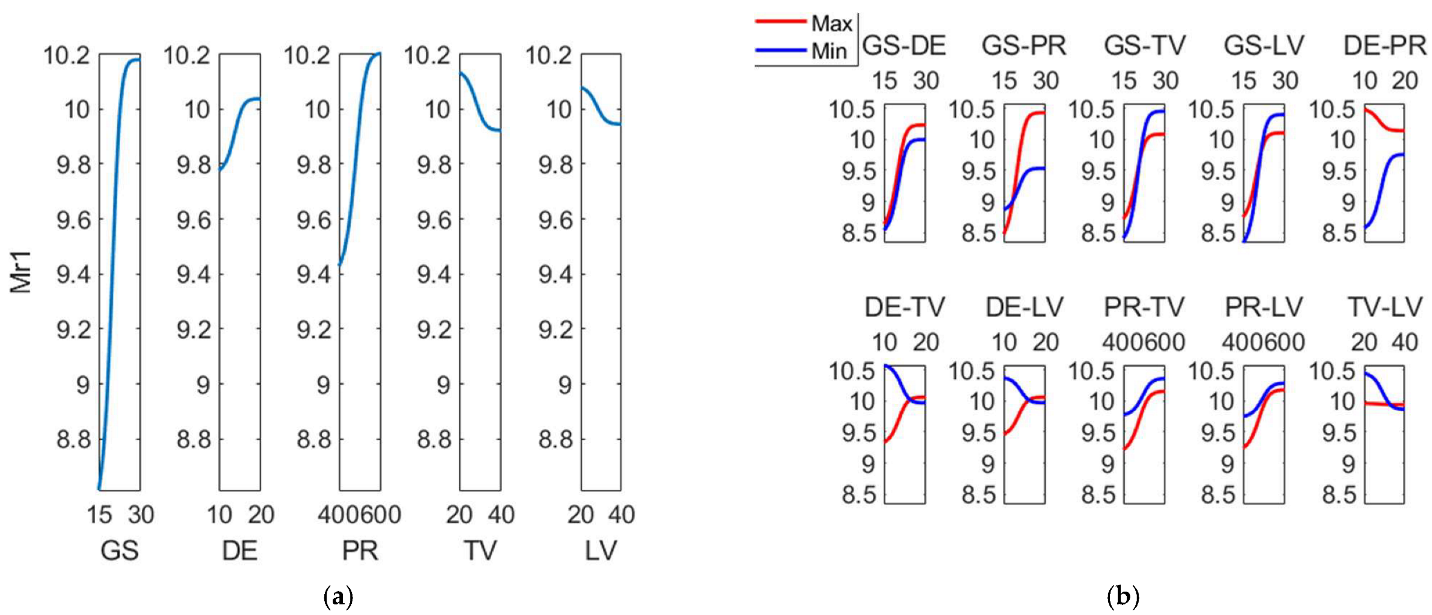
Figure 11 corresponds to the surface response plots for (Mr1) and Figure 12 depicts both the main effect plot and the interaction effects plot for (Mr1). It can be observed that the main effect for (Mr1) is grain size (GS), followed by pressure (PR). Most significant interactions correspond to GS with all the other variables, as well as DE-PR.
Figure 13 depicts the main effects and the interaction effects plot for (Mr2). As can be observed, the main effect for (Mr2) is grain size. On the other hand, most significant interactions correspond to GS-DE, GS-PR, GS-TV and GS-LV. Anderberg et al. found a great correlation between (Mr1) and (Mr2) in honing processes [38].
Figure 14 corresponds to the main effects plot and the interactions effect plot for (Rz). As with (Rk), the main factors are GS and PR, and the main interactions are those related to GS.
Figure 15 corresponds to the main effects plot and the main interactions plot for (Rsk). It can be observed that the main effect for (Rsk) is grain size, followed distantly by pressure. Most significant interactions correspond to those of (GS) with all the other variables. In this work, (Rsk) increases with grain size. Conversely, in the grinding processes of Inconel, (Rsk), a larger grit size results in lower (more negative) (Rsk) values [39]. In polishing operations of copper parts, the corresponding areal skewness parameter (Ssk) decreases slightly with grain size up to a certain grain size value from which it increases [40].
Figure 16 shows the main effects plot and the main interactions plot for skewness kurtosis (Rku). Main effect for (Rku) is grain size, followed by pressure. Most significant interactions correspond to (GS) with all the other variables. As a general trend, in grinding processes kurtosis is more related to grain size than to the cutting conditions [41]. In this work, (Rku) decreases with grain size. Conversely, in grinding processes of Inconel, (Rku) increases with grain size [39]. In polishing operations of copper parts, the corresponding areal kurtosis parameter (Sku) decreases slightly with grain size up to a certain grain size value and then increases [40].
The main effects plot and the main interactions plot for (RSm) can be observed in Figure 17. Contrary to what happens to the rest of the responses, in this case main effect is tangential velocity (TV), followed by linear velocity (LV) and by grain size (GS). Main interaction effects correspond to those related to TV, like GS-TV, DE-TV, PR-TV and TV-LV. Parameter (RSm) was reported to decrease after belt grinding and superfinishing (with honing stones) [15].

4. Conclusions

In this present study an analysis of all five bearing area parameters (Rpk), (Rk), (Rvk), (Mr1) and (Mr2), and additionally (Rz), (Rsk), (Rku) and (RSm) have been analyzed by using fuzzy inference systems and artificial neural fuzzy inference systems, where five design parameters were considered as input variables (GS, DE, PR, TV, LV).
It was found that the models thus obtained allow predicting the behavior of the response variables with a high degree of accuracy within the current range of variation and parameters considered.
On the other hand, it was shown that in all response variables except for (RSm) the main affecting parameter is grain size (GS), which could be related to the fact that the finishing honing operation is the main objective of this study. Grain Size of 30 and pressure of 600 N/cm2 lead to the highest values of core roughness (Rk) and reduced valley depth (Rvk), which were 1.741 µm and 0.884 µm, respectively. On the other hand, the maximum peak-to-valley height of the profile parameter (Rz) so obtained was 4.44 µm, which is close to the maximum value of 4.47 µm.
On the other hand, values of the grain size equal to 15 and density equal to 20, along with pressure 600 N/cm2 and both tangential and linear speed of 20 m/min and 40 m/min, respectively, lead to the minimum values of core roughness, reduce peak height, reduced valley depth and maximum peak-to-valley height of the profile within a sampling length; these were, respectively, 0.141 µm, 0.065 µm, 0.142 µm, and 0.584 µm.
In general, it has been observed that the main parameter affecting the results in this study, except for (RSm), is grain size (GS), followed by pressure (PR). As for the interactions, the most significant ones are related to the (GS) parameter, for example, GS-DE, GS-PR, GS-TV and GS-LV for both the case of (Rk) and (Rpk).
With regard to (RSm), the main affecting parameter is tangential velocity (TV), followed by linear velocity (LV) and by grain size (GS). A low value of the grain size equal to 15 along with 40 m/min for the tangential velocity and 20 m/min for the linear velocity led to a value of (RSm) equal to 31.468 µm, and contrarily, a value of the grain size of 30 along with 20 m/min for the tangential velocity and 40 m/min for the linear velocity led to the maximum value of (RSm), which was 75.64 µm. Moreover, main interaction effects correspond to those related to (TV), like GS-TV, DE-TV, PR-TV and TV-LV.
Future research will include selecting different finishing conditions. On the other hand, different tools will be included.

Author Contributions

Conceptualization, I.B.-C. and P.S.; methodology, I.B.-C. and C.J.L.-P.; software, C.J.L.-P. and P.S. All authors have read and agreed to the published version of the manuscript.

Funding

Financial support of these studies from Gdańsk University of Technology by the DEC-6/2021/IDUB/IV.2/EUROPIUM application number 035506 grant under the IDUB—‘Excellence Initiative—Research University’ program is gratefully acknowledged.

Data Availability Statement

Data available on request.

Acknowledgments

The authors would like to thank the company Honingtec S.A. and Alejandro Domínguez-Fernández for their help with the experimental tests.

Conflicts of Interest

The authors declare no conflict of interest.

References

  1. Mezghani, S.; Demirci, I.; Yousfi, M.; El Mansori, M. Mutual influence of crosshatch angle and superficial roughness of honed surfaces on friction in ring-pack tribo-system. Tribol. Int. 2013, 66, 54–59. [Google Scholar] [CrossRef] [Green Version]
  2. Jocsak, J.; Li, Y.; Tian, T.; Wong, V.W. Modeling and optimizing honing texture for reduced friction in internal combustion engines. SAE Tech. Pap. 2006, 115, 335–347. [Google Scholar]
  3. Baby, A.K.; Rajendrakumar, P.K.; Lawrence, K.D. Influence of honing angle on tribological behaviour of cylinder liner–piston ring pair: Experimental investigation. Tribol. Int. 2021, 167, 107355. [Google Scholar] [CrossRef]
  4. Buj-Corral, I.; Rodero-de-Lamo, L.; Marco-Almagro, L. Optimization and Sensitivity Analysis of the Cutting Conditions in Rough, Semi-Finish and Finish Honing. Materials 2021, 15, 75. [Google Scholar] [CrossRef] [PubMed]
  5. Kanthababu, M.; Shunmugam, M.S.; Singaperumal, M. Identification of significant parameters and appropriate levels in honing of cylinder liners. Int. J. Mach. Mach. Mater. 2009, 5, 80. [Google Scholar] [CrossRef]
  6. Barros, G.H.C.; Schramm, C.R.; Franco, S.D.; Arantes, L.J.; Arencibia, R.V. Effect of grain size and number of strokes on Rk parameters and emptiness coefficient in honing process. Int. J. Adv. Manuf. Technol. 2019, 103, 3717–3734. [Google Scholar] [CrossRef]
  7. Sadizade, B.; Araee, A.; Bavil Oliaei, S.N.; Farshi, V.R. Plateau honing of a diesel engine cylinder with special topography and reasonable machining time. Tribol. Int. 2020, 146, 106204. [Google Scholar] [CrossRef]
  8. Ma, S.; Liu, Y.; Wang, Z.; Wang, Z.; Huang, R.; Xu, J. The Effect of Honing Angle and Roughness Height on the Tribological Performance of CuNiCr Iron Liner. Metals 2019, 9, 487. [Google Scholar] [CrossRef] [Green Version]
  9. Deepak Lawrence, K.; Shanmugamani, R.; Ramamoorthy, B. Evaluation of image based Abbott–Firestone curve parameters using machine vision for the characterization of cylinder liner surface topography. Measurement 2014, 55, 318–334. [Google Scholar] [CrossRef]
  10. Pawlus, P.; Cieslak, T.; Mathia, T. The study of cylinder liner plateau honing process. Spec. Issue 1st Int. Conf. Abras. Process. 2009, 209, 6078–6086. [Google Scholar] [CrossRef]
  11. Stout, K.J.; Davis, E.J.; Sullivan, P.J. Honed Surfaces. In Atlas of Machined Surfaces; Springer: Dordrecht, The Netherlands, 1990; pp. 195–210. [Google Scholar]
  12. Kang, J.; Lu, Y.; Yang, X.; Zhao, X.; Zhang, Y.; Xing, Z. Modeling and experimental investigation of wear and roughness for honed cylinder liner during running-in process. Tribol. Int. 2022, 171, 107531. [Google Scholar] [CrossRef]
  13. Pawlus, P.; Reizer, R.; Wieczorowski, M. Characterization of the shape of height distribution of two-process profile. Meas. J. Int. Meas. Confed. 2019, 153, 107387. [Google Scholar] [CrossRef]
  14. Buj-Corral, I.; Álvarez-Flórez, J.; Domínguez-Fernández, A. Acoustic emission analysis for the detection of appropriate cutting operations in honing processes. Mech. Syst. Signal Process. 2018, 99, 873–885. [Google Scholar] [CrossRef]
  15. Grzesik, W.; Rech, J.; Wanat, T. Surface finish on hardened bearing steel parts produced by superhard and abrasive tools. Int. J. Mach. Tools Manuf. 2007, 47, 255–262. [Google Scholar] [CrossRef]
  16. Cherguy, O.; Elicegui, U.; Cabanettes, F.; Han, S.; Cici, M.; Pascal, H.; Rech, J. Effect of abrasive grains size on surface integrity during belt finishing of a 27MnCr5 carburized steel. Procedia CIRP 2022, 108, 305–310. [Google Scholar] [CrossRef]
  17. Pawlus, P.; Reizer, R.; Żelasko, W. Two-Process Random Textures: Measurement, Characterization, Modeling and Tribological Impact: A Review. Materials 2021, 15, 268. [Google Scholar] [CrossRef]
  18. Lalwani, V.; Sharma, P.; Pruncu, C.I.; Unune, D.R. Response surface methodology and artificial neural network-based models for predicting performance of wire electrical discharge machining of inconel 718 alloy. J. Manuf. Mater. Process. 2020, 4, 44. [Google Scholar] [CrossRef]
  19. Mirifar, S.; Kadivar, M.; Azarhoushang, B. First steps through intelligent grinding using machine learning via integrated acoustic emission sensors. J. Manuf. Mater. Process. 2020, 4, 35. [Google Scholar] [CrossRef]
  20. Buj-Corral, I.; Sivatte-Adroer, M.; Llanas-Parra, X. Adaptive indirect neural network model for roughness in honing processes. Tribol. Int. 2019, 141, 105891. [Google Scholar] [CrossRef]
  21. Aamir, M.; Tu, S.; Tolouei-Rad, M.; Giasin, K.; Vafadar, A. Optimization and modeling of process parameters in multi-hole simultaneous drilling using taguchi method and fuzzy logic approach. Materials 2020, 13, 680. [Google Scholar] [CrossRef] [Green Version]
  22. Alajmi, M.S.; Almeshal, A.M. Prediction and Optimization of Surface Roughness in a Turning Process Using the ANFIS-QPSO Method. Materials 2020, 13, 2986. [Google Scholar] [CrossRef] [PubMed]
  23. Shivakoti, I.; Rodrigues, L.L.R.; Cep, R.; Pradhan, P.M.; Sharma, A.; Kumar Bhoi, A. Experimental Investigation and ANFIS-Based Modelling During Machining of EN31 Alloy Steel. Materials 2020, 13, 3137. [Google Scholar] [CrossRef] [PubMed]
  24. Nguyen, D.T.; Yin, S.; Tang, Q.; Son, P.X.; Duc, L.A. Online monitoring of surface roughness and grinding wheel wear when grinding Ti-6Al-4V titanium alloy using ANFIS-GPR hybrid algorithm and Taguchi analysis. Precis. Eng. 2019, 55, 275–292. [Google Scholar] [CrossRef]
  25. ISO ISO 6106.2013; Abrasive Products—Checking the Grain Size of Superabrasives. International Organization for Standardization: Geneva, Switzerland, 2013.
  26. ISO ISO 6104:2005; Superabrasive products—Rotating Grinding Tools with Diamond or Cubic Boron Nitride—General Survey, Designation and Multilingual Nomenclature. International Organization for Standardization: Geneva, Switzerland, 2005.
  27. Luis Pérez, C.J. A proposal of an adaptive neuro-fuzzy inference system for modeling experimental data in manufacturing engineering. Mathematics 2020, 8, 1390. [Google Scholar] [CrossRef]
  28. The MathWorks Inc. Fuzzy Logic ToolboxTMUser’s Guide© Copyright 1995–2020; The MathWorks, Inc.: Natick, MA, USA, 2020. [Google Scholar]
  29. Versaci, M.; Calcagno, S.; Cacciola, M.; Morabito, F.C.; Palamara, I.; Pellicanò, D. Chapter 6: Standard Soft Computing Techniques for Characterization of Defects in Nondestructive Evaluation. In Ultrasonic Nondestructive Evaluation Systems. Industrial Application Issues; Burrascano, P., Callegari, S., Montisci, A., Ricci, M., Versaci, M., Eds.; Springer International Publishing: Cham, Switzerland, 2015; pp. 175–199. [Google Scholar]
  30. Jang, J.-S.R. ANFIS: Adaptive-network-based fuzzy inference system. IEEE Trans. Syst. Man. Cybern. 1993, 23, 665–685. [Google Scholar] [CrossRef]
  31. Bhushan, B. Modern Tribology Handbook: Volume One: Principles of Tribology; CRC Press: Boca Raton, FL, USA, 2000; ISBN 9780849377877. [Google Scholar]
  32. Pawlus, P.; Reizer, R.; Wieczorowski, M. Analysis of surface texture of plateau-honed cylinder liner—A review. Precis. Eng. 2021, 72, 807–822. [Google Scholar] [CrossRef]
  33. Klocke, F.; Brinksmeier, E.; Weinert, K. Capability profile of hard cutting and grinding processes. CIRP Ann.-Manuf. Technol. 2005, 54, 22–45. [Google Scholar] [CrossRef]
  34. Grzesik, W.; Wanat, T. Comparative assessment of surface roughness produced by hard machining with mixed ceramic tools including 2D and 3D analysis. J. Mater. 2005, 169, 364–371. [Google Scholar] [CrossRef]
  35. Wang, W.; Li, J.; Fan, W.; Zhao, C. Belt grinding mechanism-based method for roughness profile prediction of the rail surface. J. Braz. Soc. Mech. Sci. Eng. 2022, 44, 84. [Google Scholar] [CrossRef]
  36. Buj-Corral, I.; Rodero-De-Lamo, L.; Marco-Almagro, L. Use of results from honing test machines to determine roughness in industrial honing machines. J. Manuf. Process. 2017, 28, 60–69. [Google Scholar] [CrossRef] [Green Version]
  37. Lu, Y.; Li, J.; Liang, R.; Zhang, Y.; Luo, M.; Guo, C. Investigation on the effect of honing parameters on cylindricity of engine cylinder liner. Int. J. Adv. Manuf. Technol. 2020, 111, 3111–3122. [Google Scholar] [CrossRef]
  38. Anderberg, C.; Pawlus, P.; Rosén, B.-G.; Thomas, T.R. Alternative descriptions of roughness for cylinder liner production. J. Mater. Process. Technol. 2009, 209, 1936–1942. [Google Scholar] [CrossRef]
  39. Ruzzi, R.d.S.; de Paiva, R.L.; da Silva, L.R.R.; Abrão, A.M.; Brandão, L.C.; da Silva, R.B. Comprehensive study on Inconel 718 surface topography after grinding. Tribol. Int. 2021, 158, 106919. [Google Scholar] [CrossRef]
  40. Carneiro, K.; Jensen, C.P.; Jørgensen, J.F.; Garnœs, J.; McKeown, P.A. Roughness Parameters of Surfaces by Atomic Force Microscopy. CIRP Ann. 1995, 44, 517–522. [Google Scholar] [CrossRef]
  41. Ruzzi, R.d.S.; da Silva, L.R.R.; da Silva, R.B.; da Silva Junior, W.M.; Bianchi, E.C. Topographical analysis of machined surfaces after grinding with different cooling-lubrication techniques. Tribol. Int. 2019, 141, 105962. [Google Scholar] [CrossRef]
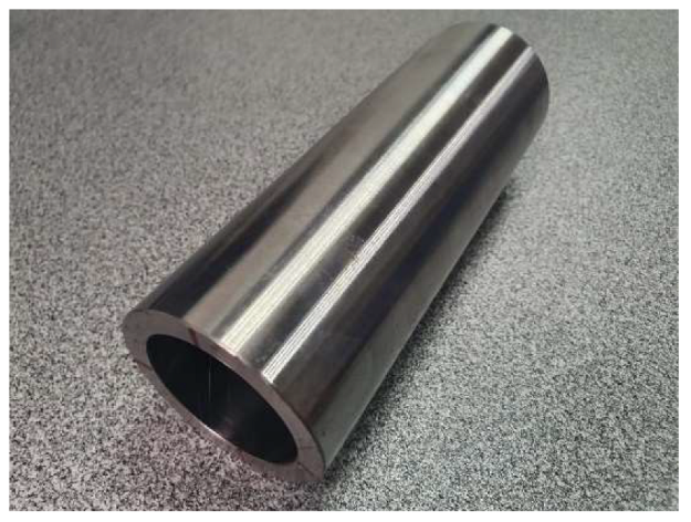
Figure 1. Steel St-52 cylinders.
Jmmp 07 00023 g001
Figure 2. cBN honing stones.
Jmmp 07 00023 g002
Figure 3. Taylor Hobson Talysurf 2 contact roughness meter.
Jmmp 07 00023 g003
Figure 4. Membership functions for fuzzification of the inputs for: (a) GS; (b) DE; (c) PR; (d) TV; (e) LV.
Jmmp 07 00023 g004
Figure 5. Output of the ANFIS model for experiment #10, in the case of Mr2.
Jmmp 07 00023 g005
Figure 6. Roughness profiles of: (a) Experiment 9, obtained with high pressure of 600 N/cm2; (b) Experiment 11, obtained with low pressure of 400 N/cm2.
Jmmp 07 00023 g006
Figure 7. Response surface for (Rk (µm)) versus each pair of input variables while the rest are kept at their central values, using the ANFIS developed for (Rk): (a) GS and DE; (b) GS and PR; (c) GS and TV; (d) GS and LV; (e) DE and PR; (f) DE and TV; (g) DE and LV; (h) PR and TV; (i) PR and LV; (j) TV and LV.
Jmmp 07 00023 g007aJmmp 07 00023 g007b
Figure 8. (a) Main effects plot and (b) interaction effects plot for (Rk (µm)).
Jmmp 07 00023 g008
Figure 9. (a) Main effects plot and (b) interaction effects plot for (Rpk (µm)).
Jmmp 07 00023 g009
Figure 10. (a) Main effects plot and (b) interaction effects plot for (Rvk (µm)).
Jmmp 07 00023 g010
Figure 11. Response surface for (Mr1 (%)) versus each pair of input variables while the rest are kept at their central values, using the ANFIS developed for (Mr1): (a) GS and DE; (b) GS and PR; (c) GS and TV; (d) GS and LV; (e) DE and PR; (f) DE and TV; (g) DE and LV; (h) PR and TV; (i) PR and LV; (j) TV and LV.
Jmmp 07 00023 g011aJmmp 07 00023 g011b
Figure 12. (a) Main effects plot and (b) interaction effects plot for Mr1 (%).
Jmmp 07 00023 g012
Figure 13. (a) Main effects plot and (b) interaction effects plot for (Mr2 (%)).
Jmmp 07 00023 g013
Figure 14. (a) Main effects plot and (b) interaction effects plot for Rz (µm).
Jmmp 07 00023 g014
Figure 15. (a) Main effects plot and (b) interaction effects plot for (Rsk).
Jmmp 07 00023 g015
Figure 16. (a) Main effects plot and (b) interaction effects plot for Rku.
Jmmp 07 00023 g016
Figure 17. (a) Main effects plot and (b) interaction effects plot for RSm (µm).
Jmmp 07 00023 g017
Table 1. Levels of the input variables.
Input VariablesLowCenterHigh
GS:Grain Size(ISO 6106 [25])152030
DE:Density(ISO 6104 [26])101520
PR:Pressure(N/cm2)400500600
TV:Tangential Speed(m/min)203040
LV:Linear Speed(m/min)203040
Table 2. Results of the honing tests.
#GSDEPRTVLVRkRpkRvkMr1Mr2RzRskRkuRSm
1152040020200.1750.0770.1758.38083.1680.768−1.2807.41735.558
2152060040200.2940.1000.1918.12087.1200.976−0.8176.68831.468
3152060020400.1410.0650.1428.16884.5080.584−2.06118.14559.563
4152040040400.3230.1430.2199.05087.3551.234−0.6348.47939.895
5151060020200.2310.1120.3228.19384.4851.222−2.21714.76652.478
6151040040200.1910.0800.1838.02584.3430.876−1.3339.00836.233
7151040020400.2320.1420.2648.61383.7250.923−1.1409.52656.975
8151060040400.2250.1310.2238.49084.2180.954−0.7528.25340.108
9302060020201.5520.7810.67410.77888.8753.8030.2373.59947.790
10302040040200.5880.2750.4009.88088.2052.211−0.5256.24144.748
11302040020401.0900.4930.4889.88589.4932.6600.0234.21669.445
12302060040401.7410.7500.88410.26088.9984.439−0.0253.83748.318
13301040020200.7370.4600.4669.94887.6052.504−0.0856.15755.480
14301060040201.6820.8070.75210.80889.4204.4700.1293.65139.013
15301060020401.6290.7190.75611.06089.4053.794−0.0794.01875.640
16301040040400.7570.3700.3858.18888.0002.127−0.1364.54647.088
17201550030300.5180.2800.3069.15087.4931.639−0.1934.79437.233
18201550030300.7150.3230.4119.92586.6132.104−0.1704.28250.043
19201550030300.7290.3530.4259.23387.6352.355−0.1474.78051.618
Table 3. Values of the membership functions employed to develop the FISs.
[Input1][Input2][Input3]
Name = ‘GS’
Range = [15 30]
MF1 = ‘x1’:‘gaussmf’, [4.2857 15]
MF2 = ‘x12’:‘gaussmf’, [6.4286 30]
Name = ‘DE’
Range = [10 20]
MF1 = ‘x21’:‘gaussmf’, [2.8571 10]
MF2 = ‘x22’:‘gaussmf’, [4.2857 20]
Name = ‘PR’
Range = [400 600]
MF1 = ‘x31’:‘gaussmf’, [57.1429 400]
MF2 = ‘x32’:‘gaussmf’, [85.7143 600]
[Input4][Input5]
Name = ‘TV’
Range = [20 40]
MF1 = ‘x41’:‘gaussmf’, [5.7143 20]
MF2 = ‘x42’:‘gaussmf’, [8.5714 40]
Name = ‘LV’
Range = [20 40]
MF1 = ‘x51’:‘gaussmf’, [5.7143 20]
MF2 = ‘x52’:‘gaussmf’, [8.5714 40]
Table 4. Rules of the FIS.
# Rule
1 (x1 = x11) & (x2 = x22) & (x3 = x31) & (x4 = x41) & (x5 = x51) => z1
2 (x1 = x11) & (x2 = x22) & (x3 = x32) & (x4 = x42) & (x5 = x51) => z2
3 (x1 = x11) & (x2 = x22) & (x3 = x32) & (x4 = x41) & (x5 = x52) => z3
4 (x1 = x11) & (x2 = x22) & (x3 = x31) & (x4 = x42) & (x5 = x52) => z4
5 (x1 = x11) & (x2 = x21) & (x3 = x32) & (x4 = x41) & (x5 = x51) => z5
6 (x1 = x11) & (x2 = x21) & (x3 = x31) & (x4 = x42) & (x5 = x51) => z6
7 (x1 = x11) & (x2 = x21) & (x3 = x31) & (x4 = x41) & (x5 = x52) => z7
8 (x1 = x11) & (x2 = x21) & (x3 = x32) & (x4 = x42) & (x5 = x52) => z8
9 (x1 = x12) & (x2 = x22) & (x3 = x32) & (x4 = x41) & (x5 = x51) => z9
10  (x1 = x12) & (x2 = x22) & (x3 = x31) & (x4 = x42) & (x5 = x51) => z10
11  (x1 = x12) & (x2 = x22) & (x3 = x31) & (x4 = x41) & (x5 = x52) => z11
12  (x1 = x12) & (x2 = x22) & (x3 = x32) & (x4 = x42) & (x5 = x52) => z12
13  (x1 = x12) & (x2 = x21) & (x3 = x31) & (x4 = x41) & (x5 = x51) => z13
14  (x1 = x12) & (x2 = x21) & (x3 = x32) & (x4 = x42) & (x5 = x51) => z14
15  (x1 = x12) & (x2 = x21) & (x3 = x32) & (x4 = x41) & (x5 = x52) => z15
16  (x1 = x12) & (x2 = x21) & (x3 = x31) & (x4 = x42) & (x5 = x52) => z16
Disclaimer/Publisher’s Note: The statements, opinions and data contained in all publications are solely those of the individual author(s) and contributor(s) and not of MDPI and/or the editor(s). MDPI and/or the editor(s) disclaim responsibility for any injury to people or property resulting from any ideas, methods, instructions or products referred to in the content.