Modeling Grinding Processes—Mesh or Mesh-Free Methods, 2D or 3D Approach?

Abstract

The objectives of this study are mainly two: (1) to validate whether a single grain scratch process can be modeled in two dimensions under the assumption of plane strain, and (2) to select the best discretization approach to model a single grain scratch process. This paper first focuses on the simulation of the orthogonal cutting process (aluminum alloy A2024 T351) using two mesh-based discretization approaches, the pure Lagrangian method (LAG) and the arbitrary Lagrangian–Eulerian method (ALE), and two particle-based approaches, the particle finite element method (PFEM) and smooth particle hydrodynamics (SPH), for both positive and negative rake angles. Benchmarking of the orthogonal cutting models at a rake angle of $\gamma ={20}^{\circ }$ is performed with the results of the process forces (cutting and passive forces) of a turning experiment from the literature. It is shown that all models are able to predict the cutting forces, but not the passive force. The orthogonal cutting model is further extended to simulate the cutting mechanism with negative rake tool geometries typically found in grinding and single grit scratching processes. The effects of the negative rake angles on the discretization approaches are studied. The calculated process forces are also compared to the measurements of the single grit scratch process performed at our laboratory. The 2D orthogonal cutting models significantly overestimate the process forces. One of the reasons why the orthogonal 2D cutting model is inadequate is that it cannot describe the complex mechanisms of material removal such as rubbing, plowing, and cutting. To account for these phenomena in LAG, ALE, and SPH discretization approaches, a 3D scratch model is developed. When comparing the process forces of the 3D model with the experimental measurements, all three discretization approaches show good agreement. However, it can be seen that the ALE model most closely matches the process forces with the experimental results. Finally, the ALE 3D scratch model was subjected to sensitivity analysis by changing the cutting speed, the depth of cut and the tool geometry. The results clearly show that the ALE method not only predicts the process forces and form the trends observed in the scratching experiments, but also predicts the scratch topography satisfactorily. Hence, we conclude that a 3D model is necessary to describe a scratch process and that the ALE method is the best discretization method.

1. Introduction

Simulation of dynamic machining processes by simplifying the real system is commonly used to predict machine behavior and understand the influence of machining parameters on the process. With advances in technology and the increasing availability of computing power, solving complex problems such as the interaction between abrasive grains and workpieces has become much easier [1,2,3,4,5]. Since grinding is one of the most complex machining processes [6], there is no universal model to comprehensively predict the machining behavior in terms of grinding forces, material removal, and surface finish [1,7,8]. Although there are different types of models, their validity is generally limited to specific process conditions or single effects. Empirical models or semi-empirical models are widely used because they take into account many application-specific influences. However, because they are based on experimental studies, they are valid only for the parameter settings tested. The advantage of regression analysis models [8] and neural network models [9,10,11] is the speed of the simulation; however, a physical meaning of the model is often not possible. Combinations of physical models and machine learning algorithms might help to overcome this issue [11,12]. In contrast, physics-based descriptions need a precise knowledge of the ongoing effects and models that can mathematically describe the phenomena. For a single grain engagement, Wang et al. could analytically solve for the elastic stress distribution and qualitatively predict different types of cracks [13]. In contrast, Setti et al. focused on the transition between plowing and cutting conditions and determined the minimum dynamic chip thickness values required by a kinematic simulation [14].

Often finite element methods are used for grinding models, even though there are technical limitations in developing a model that represents all the details such as material removal phenomena and practical difficulties in identifying model parameters [15,16]. Due to computational limitations, Zhao et al. only focused on the interaction on one single grain in contact with a representative volume element (100 µm × 100 µm × 100 µm) of the composite material 50 vol% SiCp/Al to evaluate the mechanism of surface defect formation [17]. For this purpose, they included effects of the particle–matrix interface behavior in a model of the 3D microstructure. To predict the temperature distribution during creep feed grinding, Orthega et al. simplified the grain engagement by a simplified geometric contact area but precisely modeled the heat flows in the workpiece, grinding wheel, chips, and cooling lubricant [18].

A well-designed simulation model of the grinding process could significantly reduce the cost of experiments and optimize the process [19]. A well-developed physical model can also help to successfully determine the behavior of the grinding process based on workpiece properties, material removal mechanisms, and tool wear. In addition, these simulations provide some invaluable information, such as stresses, strains, strain rates, and temperature gradients, that are otherwise very difficult to determine through experimental investigations [1,20,21]. Several studies on numerical simulations of machining processes under orthogonal cutting conditions and assuming plane strains were found in the literature [22,23,24,25,26]. Most of these simulations were performed using mesh-based methods; however, these simulations are prone to mesh distortions that can potentially lead to simulation failures. Mesh-free and particle-based methods are potential alternatives to mesh-based methods that overcome the previously mentioned challenge of mesh distortion [4]. Eder et al. compared three different mesh-free methods on length scales in the range of almost four orders of magnitude and found similar results in material removal rates and roughness values related to the size of the grain [21]. Despite the advantages of representable length scales and mesh-free description, mesh-free methods require more computational effort, and their accuracy in calculating process forces needs to be evaluated [27,28,29].

To study the performance of several discretization approaches and their ability to describe the material removal mechanisms occurring during grinding, a single grain scratch model is investigated. The setup reduces complexity and helps validate the models with simple scratch tests performed in our laboratory. Our goal is to identify to which extent a single grain scratching process and, hence, a grinding process can be described by a two-dimensional model and to propose the most appropriate discretization approach from the two commonly used mesh-based approaches (pure Lagrangian (LAG) and arbitrary Lagrangian–Eulerian (ALE)) and the two particle-based approaches (particle finite element method (PFEM) and smooth particle hydrodynamics (SPH)).

Section 2 describes characteristics of the four approaches and the simulation flow with modeling framework, material model, and contact model. This is followed by Section 3, which describes single grain scratch experiments performed at our laboratory to evaluate the results of the final 3D simulations. A 2D orthogonal cutting model with the four discretization approaches, LAG, ALE, SPH, and PFEM, is introduced in Section 4 to primarily describe the cutting mechanism. The simulation results are compared to the literature regarding orthogonal cutting. A 3D scratch model is finally developed to describe rubbing, plowing, and cutting mechanisms typically encountered in a grinding/single grain scratch process. The discretization approaches LAG, ALE, and SPH are used in the development of a 3D scratch model; PFEM is not considered in the scope of this study because the PFEM code for the simulation of oblique cutting is still under development. The simulation results of process forces and scratch topography are compared with experiments conducted in our laboratory and are explained in detail in Section 5. Section 6 finally summarizes the most important findings.

2. Simulation Procedure

In this section, we first give a brief overview of the used mesh-based (LAG, ALE) and mesh-free (SPH, PFEM) approaches. They were used to develop a 2D orthogonal cutting model (LAG, ALE, SPH, and PFEM) and a 3D scratch model (LAG, ALE, and SPH) for this study. MACH-PFEM, an implicit code developed by the authors themselves in Matlab^®, was used for the PFEM model [26,30]. For all other models, Abaqus/Explicit 2019 was chosen from the many commercial FEM software suites available (Abaqus, Ansys, Ls-Dyna, Deform, AdvantEdge) because it provides almost all discretization approaches studied in this work. The availability of the different discretization approaches (LAG, ALE, and SPH) makes it easy to compare them and to determine their advantages and disadvantages. This section also includes information on the choice of plasticity material model, damage model, and friction contact model used in the different discretization approaches.

2.1. Introduction to Simulation Approaches Used

The Lagrangian approach (LAG) has already been applied to numerical modeling of machining processes assuming orthogonal cutting and plane strain conditions [1,20,31]. The displacement vector follows the individual material points in the simulation. Normally, this approach is not able to follow large deformations, which may lead to simulation errors. Nevertheless, some feasible solutions have been implemented in [32,33,34], namely, element deletion and adaptive remeshing [1,35,36], although the disadvantage of the element deletion technique is the reduction of material mass. In the case of adaptive remeshing, the mapping of internal variables from an old mesh to a new mesh can lead to discrepancies in the numerical results of the simulation.

As a further development, in the arbitrary Lagrangian–Eulerian (ALE) approach, the mesh is neither bound to a fixed domain (Eulerian) nor moves together with the material points (LAG). This approach aims to maintain the mesh topology and prevent the splitting of the mesh elements. The relocation of the mesh’s node positions is performed using a mesh smoothing algorithm [37,38]. This algorithm prevents the mesh distortion and hourglass effect. Despite the fact that the ALE method is computationally efficient, its accuracy depends on the underlying mesh and the chosen smoothing algorithm [31,32].

In contrast to the mesh-based methods, the mesh-free methods fundamentally differ in their principle. In the smooth particle hydrodynamics (SPH) [39,40] method, the material domain is represented by spheres. A strong particle–particle connection represents a solid region, while a weak particle–particle connection represents fluids. The SPH method calculates a physical quantity of one particle based on the physical quantity of the neighboring particle and that of its own particle by using a weighted function. The weighted function takes into account the radius of the particle and the smoothing lengths [41]. Due to the breakable bonds between the particles, a failure criterion becomes unnecessary. As a result of the loss of cohesion between the particles, material separation occurs.

A further particle-based method is the particle finite element method (PFEM), which was first described by [42] for fluid–structure interaction problems. It is a combination of the advantages of discrete modeling techniques and continuum-based methods [42]. Therefore, it is suitable for describing large strain deformation problems, such as in metal cutting [26,30]. PFEM contradicts the classical finite element approximations by calculating the deformation of a body based on the underlying particle quantity. At the end of each time step, a mesh is approximated using the centers of the particles as nodes. A robust and fast algorithm for finding a new mesh is essential. In this work, the Delaunay tessellation method was chosen to connect the particles at each time step and generate a new mesh [43]. The PFEM simulation represents the particles as spheres and generates an unstructured 2D mesh with triangular elements. This resulting mesh serves as a support for the differential equations to be integrated. The generated mesh is also used to identify contacts and to track free surfaces. Surface tracking is realized using the alpha-shape technique implemented in [42,44].

2.2. Material Model

During material removal in ductile materials, large plastic strains and large deformation rates occur in the workpiece material. During grinding/scratching, complicated material removal mechanisms such as rubbing, plowing, and cutting appear. A material model describing such material behavior is the Johnson–Cook material model [45,46], with its mathematical description of the effective von Mises stress $\overline{\sigma }$:

$$\overline{\sigma }=\underset{f_1}{\underbrace{[A+B{\left(\epsilon \right)}^n]}}·\underset{f_2}{\underbrace{\left[1+Cln\left(\frac{\dot{\epsilon }}{{\dot{\epsilon }}_0}\right)\right]}}·\underset{f_3}{\underbrace{\left[1-{\left(\frac{T-T_{room}}{T_{melt}-T_{room}}\right)}^m\right]}}.$$

(1)

The effective von Mises stress is the product of components describing strain hardening ($f_1$) as a function of strain $\epsilon$, strain rate sensitivity ($f_2$) as a function of strain rate $\dot{\epsilon }$, and thermal softening ($f_3$) as a function of temperature T. The material parameters A, B, C, n, m, $T_{melt}$, and the room temperature $T_{room}$ are to be specified. In the previous equation, ${\dot{\epsilon }}_0$ represents the reference strain rate. In this work, the material parameters for A2024 T351 are taken from [32], as shown in

Table 1. Johnson–Cook material parameters, damage coefficients, and fracture toughness properties of A2024-T351, taken from [32].

Johnson–Cook material parameters
Initial yield strength	A	MPa	369
Strain hardening constant	B	MPa	684
Strengthening coefficient of strain rate	C	-	0.0083
Strain hardening coefficient	n	-	0.73
Thermal softening coefficient	m	-	1.7
Johnson–Cook damage parameters
Initial-stress-triaxiality-dependent parameter	$H_1$	-	0.13
Stress-triaxiality-dependent constant	$H_2$	-	0.13
Stress-triaxiality-dependent coefficient	$H_3$	-	1.5
Strain-rate-dependent parameter	$H_4$	-	0.011
Temperature-dependent parameter	$H_5$	-	0
Fracture toughness—mode I	$K_{IC}$	MPa$\sqrt{\mathrm{m}}$	37
Fracture toughness—mode II	$K_{IIC}$	MPa$\sqrt{\mathrm{m}}$	26
Poisson ratio	$\nu$	-	0.3
Young’s modulus	E	GPa	73

.

The Johnson–Cook damage model [46] is used in conjunction with the Johnson–Cook material model to calculate damage evolution in the 2D orthogonal cutting model and in the 3D scratch model. The plastic strain at failure ${\overline{\epsilon }}^f$

$${\overline{\epsilon }}^f=\underset{g_1}{\underbrace{\left(H_1+H_{2}exp\left(H_3\frac{{\sigma }_m}{\overline{\sigma }}\right)\right)}}·\underset{g_2}{\underbrace{\left(1+H_{4}ln\frac{\dot{\epsilon }}{{\dot{\epsilon }}_0}\right)}}·\underset{g_3}{\underbrace{\left[1-H_5{\left(\frac{T-T_{room}}{T_{melt}-T_{room}}\right)}^m\right]}}$$

(2)

is the product of the relationship between hydrostatic stress and von Mises stress ($g_1$), the relationship between strain rate and material ductility ($g_2$), and the effect of thermal softening on material ductility ($g_3$). In Equation (2), $H_1$–$H_5$ are damage parameters. In this work, we use a simplified Johnson–Cook damage model with neglected temperature-dependent effects and with the parameters fitted by [32]; see Table 1. The thermal softening on the material ductility ($H_5$) is neglected because it is quite difficult to determine this temperature-dependent parameter at high temperatures and high strain rates. Therefore, it is set to zero to simplify the comparison of the different discretization approaches. Furthermore, since the work of Johnson and Holmquist in 1989, in which the properties of 23 different materials were measured, $H_5$ was always given as 0 for aluminum. Other authors also used $H_5$ equal to zero in their work [22,23,47,48,49].

In this study, the damage evolution $\dot{D}$ is determined by the Hillerborg fracture energy model with linear softening [50]. Once the damage is initiated, the damage evolution $\dot{D}$ varies according to

$$\dot{D}=\frac{L\dot{\epsilon }}{u_f}=\frac{\dot{u}}{u_f},$$

(3)

where L is a characteristic length of the finite element and $u_f$ is the plastic displacement at failure, defined as

$$u_f=\frac{2G_f}{{\sigma }_{y0}},$$

(4)

where ${\sigma }_{y0}$ is the value of the field stress when the failure criterion is met and $G_f$ is the fracture energy. After damage initiation for $D>0$, the new yield strength value $\sigma$ and new Young’s modulus $\tilde{E}$ can be computed using $\sigma =(1-D)\tilde{\sigma }$ and $\tilde{E}=(1-D)E$. The fracture energy $G_f$, a material parameter that shows the required energy to open a unit area of crack [51], can be determined by

$$G_f=\frac{1-{\nu }^2}{E}{K_i}^2$$

(5)

for fracture mode i. In the literature, there are two types of crack development, an opening mode and a sliding mode. The fracture energy is determined by the corresponding fracture toughness ($K_{IC}$ and $K_{IIC}$) [22]. The fracture toughness of A2024 T351 aluminum for these two modes are provided in Table 1. It is to be noted that the SPH and PFEM model do employ the Hillerborg fracture energy model as the material separation occurs due to the lack of cohesion between the particle–particle connection. Hence, an additional chip separation criteria is not required in these methods.

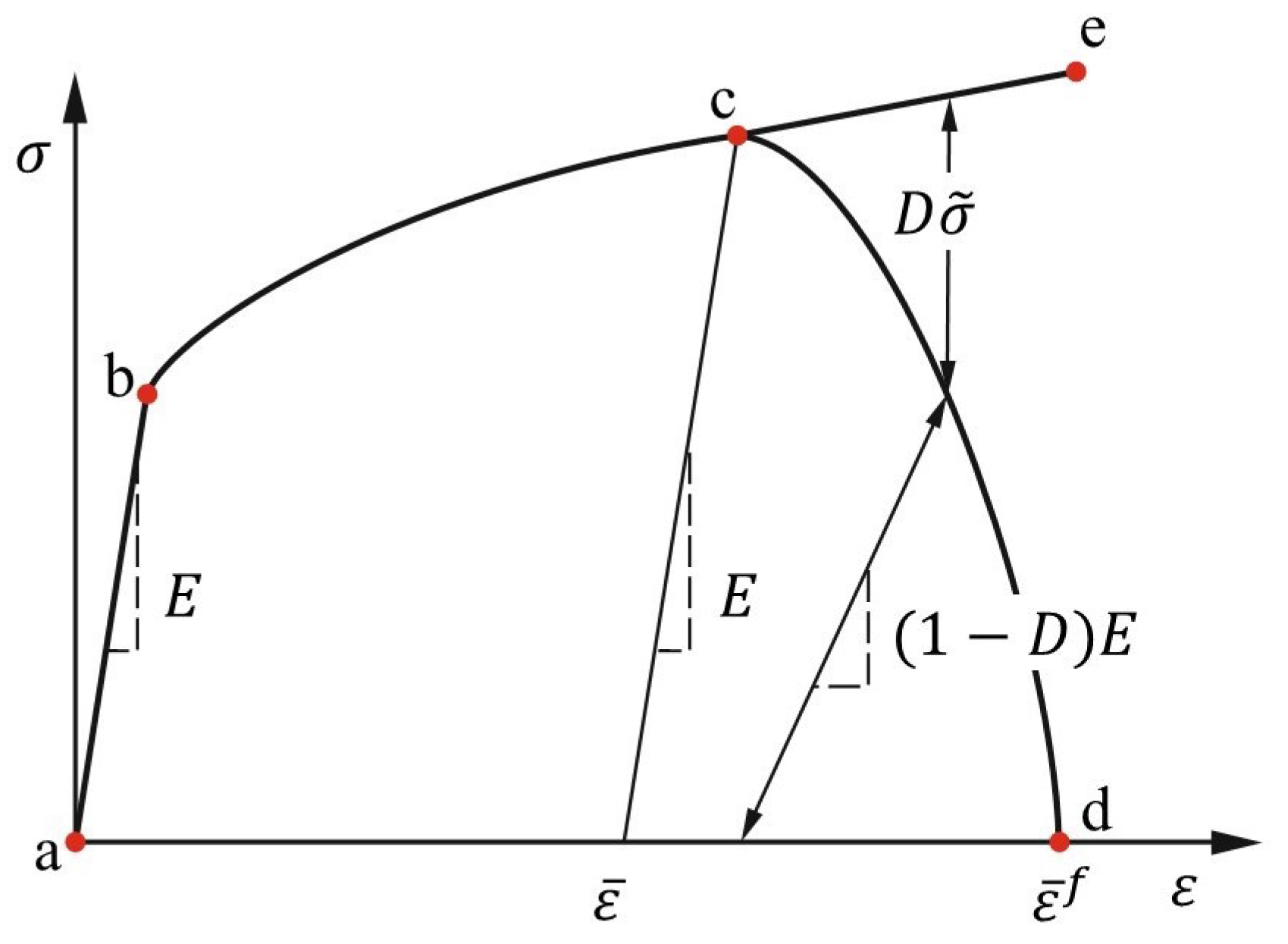
Figure 1 illustrates the Johnson–Cook material model and the Johnson–Cook damage model of an elastoplastic behavior with linear elasticity (a–b), strain hardening and thermal softening (b–c), damage initiation at (c), damage evolution (c–d), and eventually fracture (d). The stress–strain response in the absence of a damage model (c–e) is illustrated additionally.

2.3. Contact Model

During orthogonal cutting and scratching, the workpiece and tool are in constant contact. Friction occurs in the contact interface when both parts move relative to each other. A penalty-based contact algorithm defines the tool and the workpiece contact interface. Here, the master surface refers to the tool, and the slave surface to the workpiece. It is important to keep the workpiece mesh fine enough that no penetration of the tool occurs during contact.

The classic Coulomb friction law is the simplest of the friction models and is applied in the contact model. In the Coulomb friction model, the frictional stress ${\tau }_f$ is related to the normal stress ${\sigma }_n$ times a constant coefficient of friction $\mu$:

$${\tau }_f=\mu \tilde{\sigma }.$$

(6)

Both the 2D orthogonal cutting model and the 3D scratch model employ the Coulomb friction model, where the coefficient of friction is set to $\mu =0.23$ according to the investigation of [25]. Even though different coefficient of friction may be present in the contact interfaces, we chose a constant value to facilitate the comparison between the different models.

3. Experimental Setup of Scratch Experiments

For quantitative statements about the reliability of the developed models, the comparison of simulation results with measurements is indispensable. Therefore, in our laboratory we performed single grit scratch tests on samples of aluminum alloy (A2024-T351). The indenter is a diamond cone with cone angle 105^∘ and 120^∘. We kept the depth of cut constant at $a_p=$ 50 µm and varied the cutting speeds $v_c$ between 200–1000 mm/s in steps of 200 mm/s.

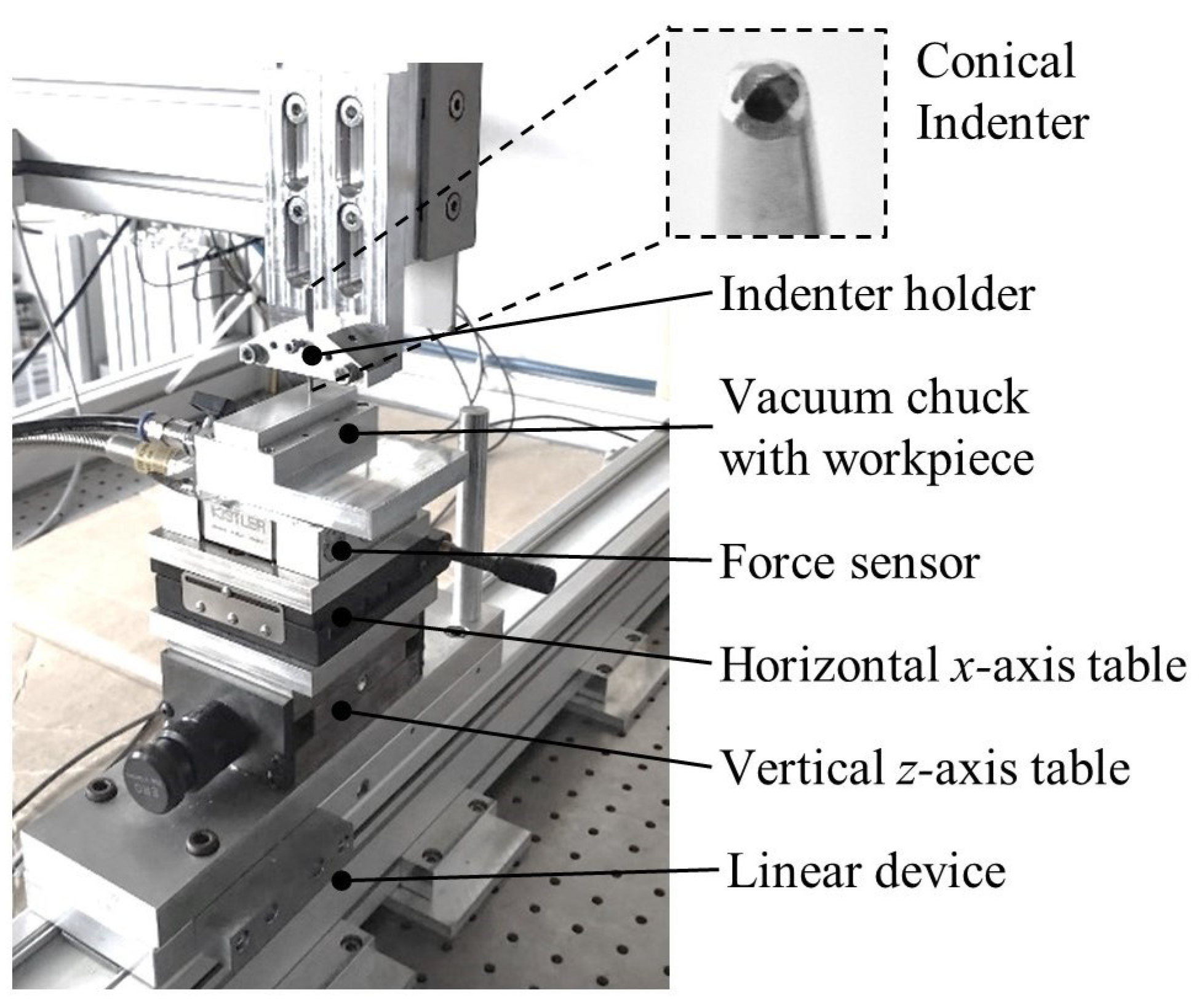
Figure 2 shows the experimental setup with a linear belt drive motion device (stroke length = 850 mm) on which a vertical z-axis table, a horizontal x-axis table, and a high-pressure vacuum chuck for the samples are mounted. With the z-axis table, the depth of cut can be adjusted in the range of 1 µm, and with the x-axis table, the scratches can be demarcated with spacing of 0.1 mm. A Kistler 3-axis force sensor (Type: 9119AA1) is placed under the vacuum chuck and workpiece to measure the process forces in the range of 0 to 400 N. The workpiece itself has the dimensions 75 mm × 20 mm × 2 mm. Above the linear device, on a vertical gantry, the specimen holder is mounted to fix the indenter.

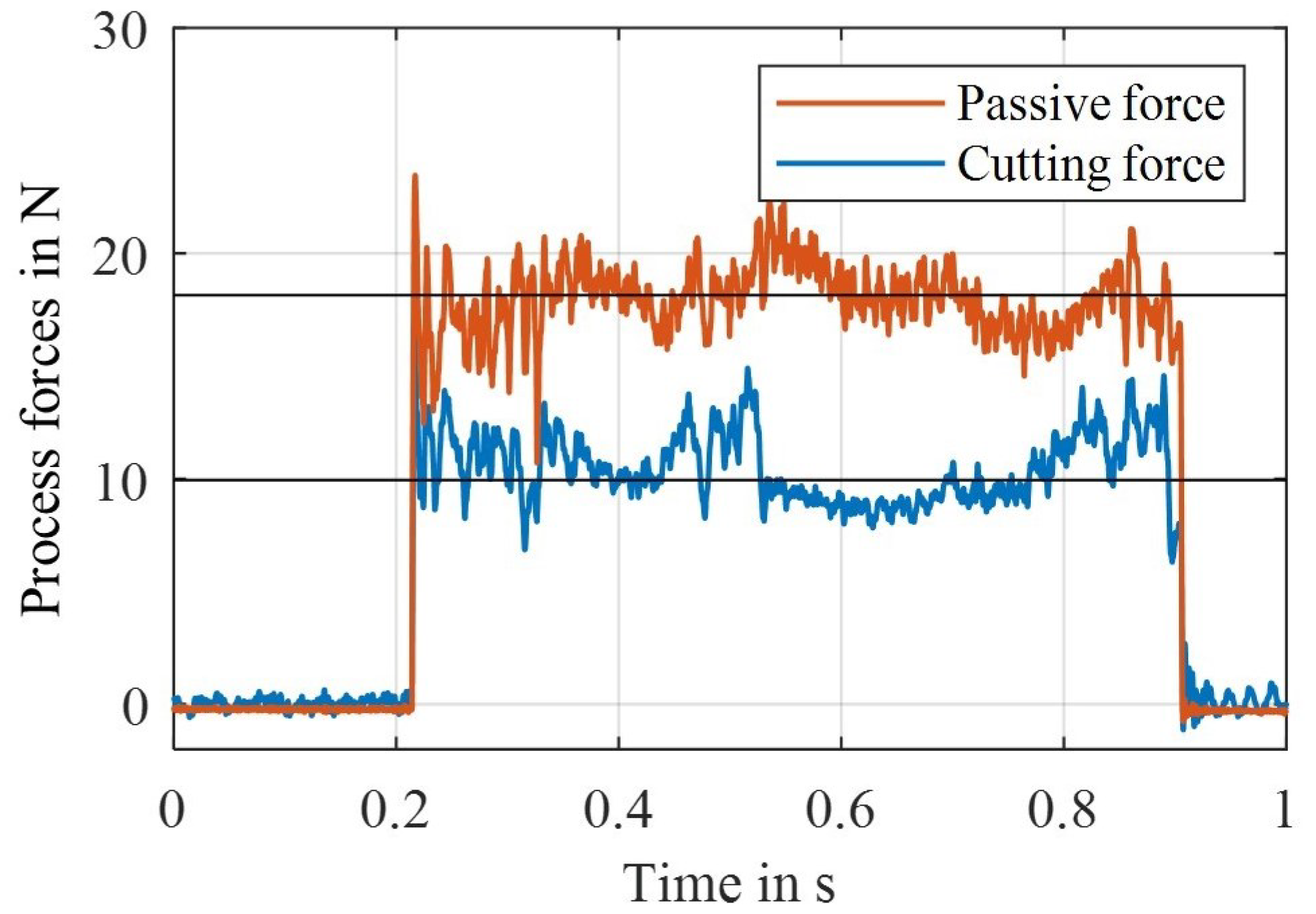
The process forces are acquired using the software suite LabView 2018, cf. Figure 3. This software also helps in controlling the cutting speed of the linear device. The sampling rate for the force measurement acquisition is set to 10,000 samples/s.

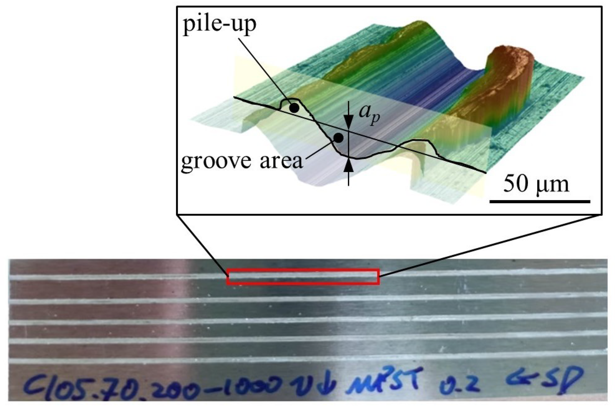
The scratch test is performed by positioning the workpiece. First, a zero position is determined and a desired cutting depth is set by adjusting the z-axis table. A distance-measuring laser is used to verify that the desired depth of cut is accurately achieved. Once the cutting depth is set, the linear device is moved to its reference position with the indenter in its fixed position. For scratching, the linear device is first accelerated to the final cutting speed, then moves at a constant speed during scratching, and is finally decelerated again. For each parameter combination (depth of cut and cutting speed), five repetitions of the single-grit scratch experiments and force measurements are performed. An example of a scratched workpiece with a conical indenter (cone angle = ${105}^{\circ }$) shows Figure 4. The surface of the workpiece was scanned after the experiments to compare the topography with simulations. The measured groove depth was found to be less than the previously specified depth of cut due to elastic deformation of the test setup. After some analysis, it was observed that the deviation is due to the combined effect of the elastic deformation of the indenter holder and workpiece holder as well as the elastic deformation of the workpiece.

Consequently, the simulations in Section 5 were performed with a reduced depth of cut with $a_{p,\mathrm{sim}}=35$ µm, which corresponds to the predefined depth of cut $a_p$ = 50 µm during experiments.

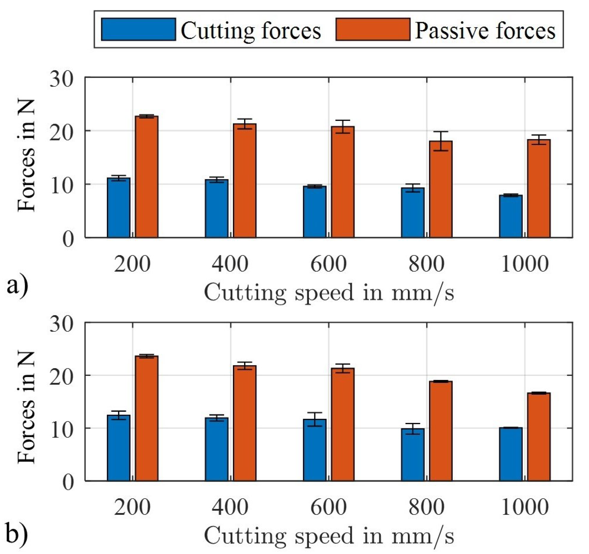
Figure 5a,b show that the measured passive forces are higher than the cutting forces for all tested speeds ($v_c$ = 200–1000 mm/s) and cone angles (${105}^{\circ }$ and ${120}^{\circ }$). The standard deviation of the passive forces and cutting forces measured are almost the same (±0.7 N), with no large deviations between the single experiments. Similarly to already published investigations [52,53], we also observed that the process forces reduce with increased cutting speed, which shows that we can reproduce major trends with the experimental setup.

The results obtained from these experimental investigations are used in the following to validate and analyze the 3D scratch models with LAG, ALE, and SPH discretization approaches.

4. Orthogonal Cutting Model as 2D Approach

In this section, the simulation framework, benchmark simulations, and study on the effect of tool rake angle $\gamma$ are described for the 2D orthogonal cutting model and the four discretization approaches: LAG, ALE, SPH, and PFEM.

4.1. Simulation Framework of 2D Cutting Model

To benchmark the 2D models we chose orthogonal cutting with a positive rake angle $\gamma$ (equivalent to a turning process), and in contrast to our experiments, a cutting speed of 3000 mm/s. The model parameters are taken from [32] and are listed in

Table 2. Parameters of the 2D orthogonal cutting models with A2024 T351 aluminum, as per [32].

Parameters of workpiece (A2024 T351 aluminum)
Young’s modulus $E_{\mathrm{wp}}$	GPa	73
Poisson ratio ${\nu }_{\mathrm{wp}}$	-	0.3
Density ${\rho }_{\mathrm{wp}}$	kg/m${}^3$	2780
Parameters of tool (high speed steel (HSS))
Young’s modulus $E_{\mathrm{tool}}$	GPa	210
Poisson ratio ${\nu }_{\mathrm{tool}}$	-	0.33
Density ${\rho }_{\mathrm{tool}}$	kg/m${}^3$	7830
Orthogonal rake angle $\gamma$	degree	20
Clearance angle $\alpha$	degree	5
Cutting edge radius r	µm	4
Depth of cut $a_p$	µm	50
Cutting speed $v_c$	mm/s	3000

. The results from our simulation are also verified with these turning experiments.

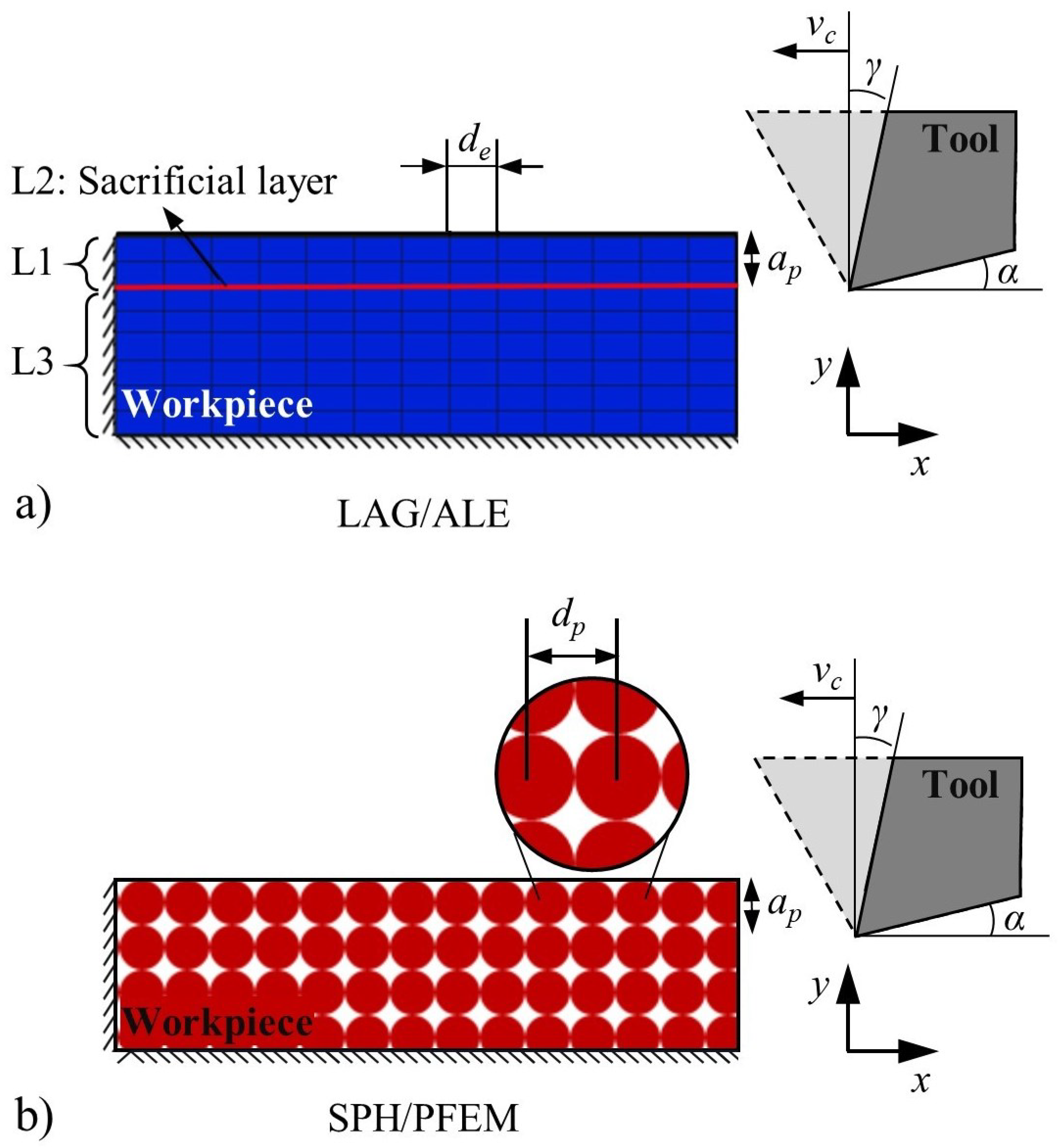
Similar to the experiment, the simulation model consists of an aluminum workpiece and a rigid tool performing an orthogonal cutting operation; see Figure 6. The LAG, ALE, SPH, and PFEM models consist of a tool (meshed body) and a workpiece (FEM/SPH elements). The tool is given an imposed motion with constant cutting velocity $v_c$ in negative x-direction, and the workpiece is fixed along its left and bottom nodes. The tool is positioned with a depth of cut $a_p=50$ µm along the y-axis (for turning, this corresponds to the feed per revolution f). The element sizes for the simulation models were previously investigated and chosen based on recommendations of [22,23,31,32] to reduce the influence of the element size or particle size and distance on the calculated reaction forces. The element discretizations $d_e$ for LAG and ALE models and the particle discretizations $d_p$ for the SPH and PFEM models were set to $d_e=d_p=3$ µm.

In the LAG and ALE simulations, the workpiece elements are divided into three layers, L1, L2, and L3, as shown in Figure 6a. The region L2 consists of a narrow line of sacrificial elements, to separate the chip region (L1) from the workpiece elements (L3). When an element in the sacrificial layer (L2) reaches the predetermined critical damage value according to the Hillerborg fracture energy model with linear softening [50], the element deletion is activated and the element is removed to prevent mesh distortion. The failure criterion is calculated based on the opening and sliding fracture modes. The failure criterion for regions L1 is calculated based on $K_{IIC}$, and for L2 elements is calculated based on $K_{IC}$ (see Equation (5)). These values were kept constant for the mesh-based models in this study.

Unlike in the LAG model, in the ALE model the chip region L1 is assigned as the ALE domain with adaptive remeshing. According to [51], in each adaptive mesh increment a new smoother mesh is created and the nodes in the domain are relocated to reduce element distortion. The higher the number of mesh sweeps, the more intense the adaptive meshing in each increment. In this study, the number of mesh sweeps was set to five. The number of increments of adaptive meshing affects the quality of the mesh and the computational efficiency. As the mesh quality is of prime importance to achieve steady-state cutting conditions, this value is set to 50,000, as in [31,51]. In the case of the LAG model, the chip region L1 is simply modeled with Lagrangian elements without activating element deletion.

In the case of the particle-based methods SPH and PFEM, no sacrificial layer is assigned, as the chip–workpiece separation occurs due to the lack of cohesion between the particle–particle connections.

4.2. Results of Benchmark Simulation in 2D

Benchmark simulations are used to validate the considered discretization approaches LAG, ALE, SPH, and PFEM, and the results are compared to the dry-turning process on aluminum alloy (A2024 T351) from [32].

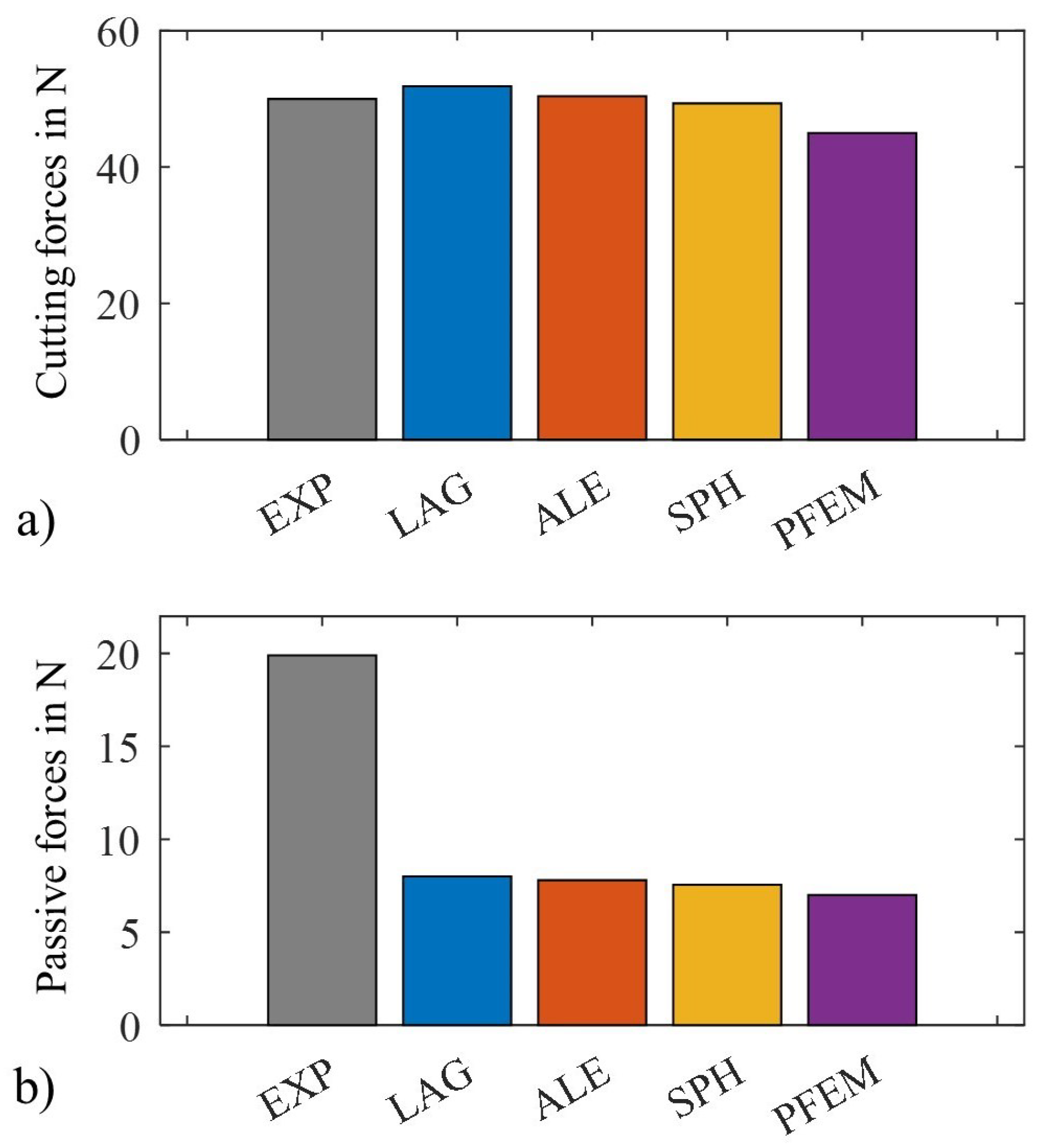
The process forces calculated from the simulation and the forces measured from [32] are illustrated in Figure 7.

In the steady state of the experiment, the measured average cutting force in the x-direction is 50 N. The LAG, ALE, and SPH methods predict the cutting force with a minor error of $1\%$. On the contrary, the PFEM approach shows a higher discrepancy in predicting the cutting force at an error of $8\%$.

Interestingly, for all discretization approaches, the passive force does not agree with the experimental results and is significantly underestimated. This miscalculation has a high error of $40\%$. For the mesh-based methods, this error can be attributed to the deletion of elements during material separation. The deletion of deformed elements occurs when a threshold value is reached and causes reduced contact between the tool and workpiece, and with this, decreased passive forces. Unlike the mesh-based methods, the mesh-free methods make use of a weighted function to determine the cohesive bonds between the particles. Within a region of influence, the cohesive forces between the particles decrease in a bell-shaped manner, which could lead to premature separation of the particles. Besides the material separation, the choice of the coefficient of friction [1,31] and the friction models could help to reduce the error in the calculation of the passive forces [54].

Nonetheless, all discretization approaches show similar results for the cutting and passive forces and are consequently considered as equivalent modeling options which need to be further examined.

4.3. Sensitivity Analysis of Negative Tool Rake Angle

To evaluate whether the four developed orthogonal 2D cutting models can simulate scratching with high negative rake angles, similarly to contact conditions occurring during grinding, we successively changed the rake angle from $\gamma ={20}^{\circ }$ (orthogonal cutting) to $\gamma =-{60}^{\circ }$ (grinding) and compared the process forces. The investigated rake angles in the range ${20}^{\circ }>\gamma >-{60}^{\circ }$ are typical in grinding. At the same time, we want to evaluate whether a two-dimensional description is sufficient for scratching with negative rake angle.

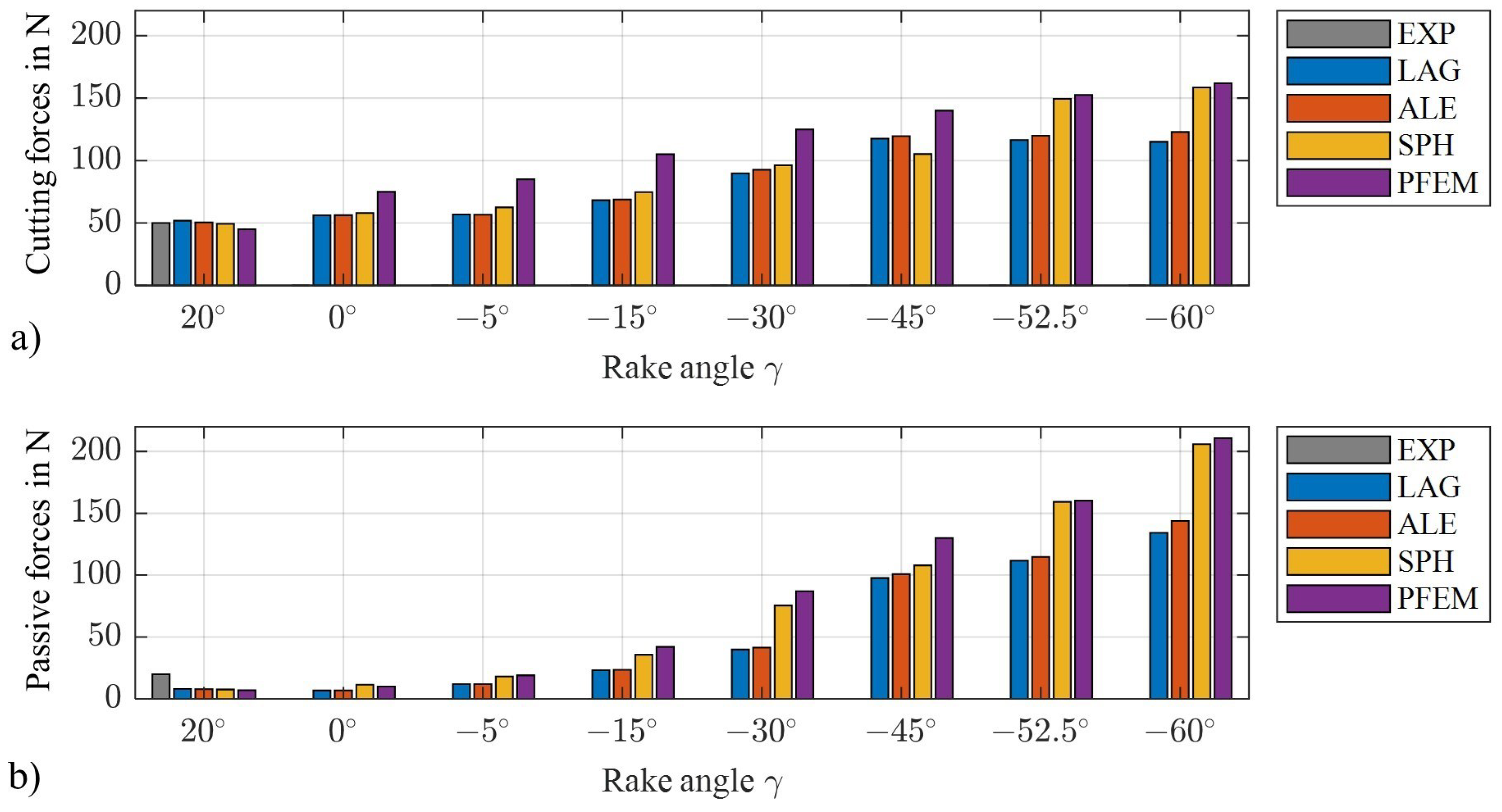
For stability reasons in the LAG and ALE simulations, the threshold value of the failure model had to be decreased for $\gamma \le -{52.5}^{\circ }$, which explains why the cutting forces do not increase further for these angles, cf. Figure 8. Comparing the results of all discretization approaches in Figure 8, it is obvious that both cutting forces and passive forces increase and the values converge more and more as the absolute value of the angle becomes higher. This trend can be attributed to the increased tool–workpiece interface for higher negative rake angles, which result in higher compressive forces on the workpiece. A similar tendency to increase process forces was found in an experimental study conducted by [55,56,57]. The comparison of the discretization approaches with each other shows that the mesh-based methods and the particle-based methods behave similarly in each case, but the particle-based methods calculate significantly higher forces. The main reason for this could be the failure model included in the mesh-based methods, for which the threshold values have to be set manually.

The verification of the process forces with scratch experiments performed at our laboratory with rake angles of $\gamma =-{52.5}^{\circ }$ and $\gamma =-{60}^{\circ }$ and various speeds (cf. Figure 5) shows that the passive forces should tend to be twice as high as the cutting forces. By observing a real single scratch experiment, it becomes clear that different interaction mechanisms prevail, which influence the process forces. The interaction between the cutting tool and the workpiece occurs in all directions, unlike the 2D cutting model where a single surface interacts with the workpiece. Spatial contact with plowing and lateral material flow, which cannot be represented in the 2D model, changes the force components. Therefore, if not only tendencies but also absolute force values are to be investigated, cutting must be modeled in 3D. Consequently, in the following section, we describe a 3D model for single grit scratching and compare the results of the LAG, ALE, and SPH approaches. The goal is to verify whether the differences in the force relation between the 2D model and the experiments are due to the fact that the problem cannot be simplified to 2D or that the material model or the friction model needs to be improved.

5. Single Grit Scratch Model as 3D Approach

A 3D single grit scratch model is developed to investigate the material flow mechanisms and to compare the geometrically more complex model with experimental studies on the grit geometry and speed of cut. Besides the analysis of the process forces, the topography is also studied. First, the simulation framework and the differences to the 2D model are explained, followed by the description of the experimental setup and results. A benchmark simulation is used to verify the models, and finally a sensitivity analysis on the indenter cone angle and the cutting speeds helps to evaluate the models with respect to predicted forces and scratch topography.

5.1. Simulation Framework of 3D Scratch Model

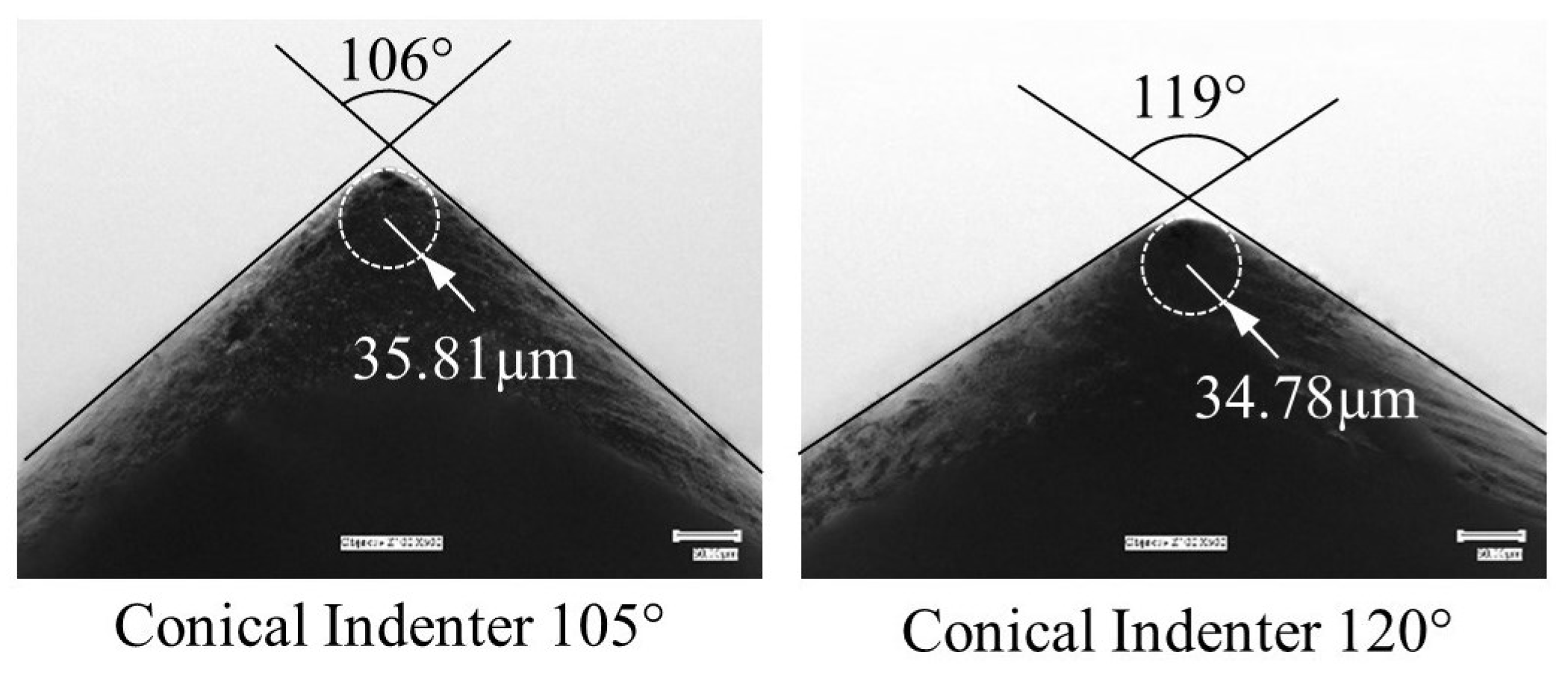
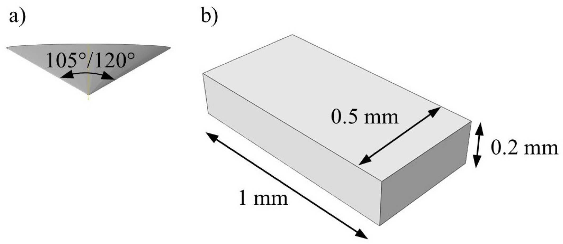
For the discretization approaches LAG, ALE, and SPH, the 3D scratch model is also developed in Abaqus/Explicit 2019. Unlike in the 2D model, the tool is now modeled as a rigid cone with cone angle 105^∘ and 120^∘ and a tool radius of 35 µm, which was calculated from microscopic images as shown in Figure 9.

The conical tool is modeled as a rigid body and meshed as coarsely as possible with an element size of about 10 µm at the apex to reduce computation time. Since the experimental tool is a diamond indenter, it is much harder than the aluminum workpiece (A2024 T351), and the simplification in the model is acceptable. A rigid point is used to tie the nodes of the tool, onto which the velocity boundary conditions are applied. Because of the reduced measured cutting depth due to elastic deformations of the experimental setup, a constant cutting depth of $a_{p,\mathrm{sim}}=35$ µm was simulated in the models, corresponding to a preset cutting depth of $a_p=50$ µm during the scratch tests in the laboratory. The cutting speeds were varied between $v_c$ = 200–1000 mm/s, analogous to the experiments.

The cuboid workpiece is modeled as a deformable body with the same material parameters for A2024 T351 aluminum as in the 2D model; see Table 2. Figure 10 shows the dimensions of the workpiece with 1 mm × 0.5 mm × 0.2 mm. In the LAG and ALE models, unlike the 2D model, there is no sacrificial layer included. The energy-based failure criterion (calculated based on $K_{IIC}$) and the Johnson–Cook material and damage model are assigned to all workpiece elements, as described in Section 2.2. In case of the SPH methods, no failure criterion is applied, as the material removal takes place based on the lack of cohesion between the particles.

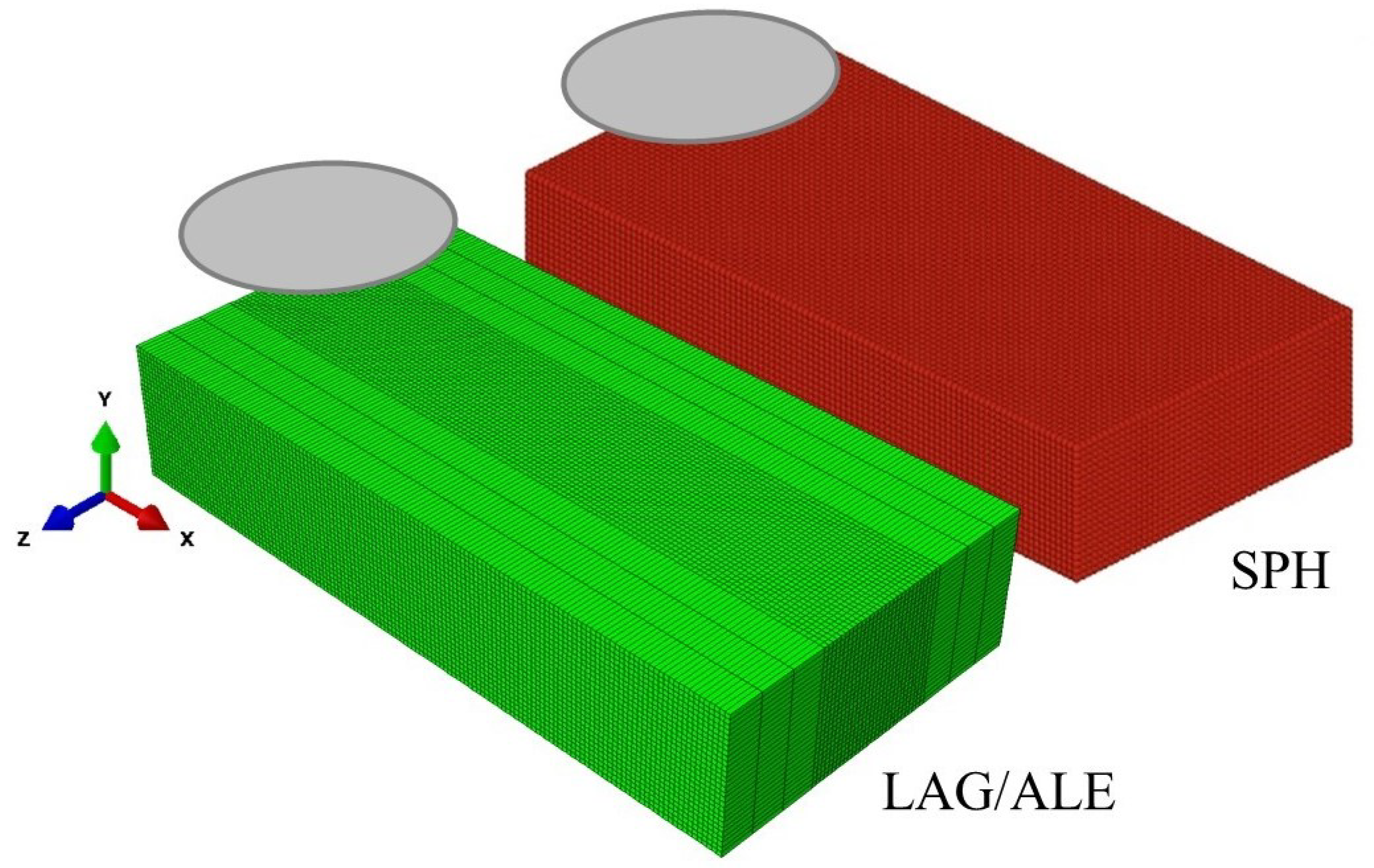
Figure 11 shows the discretized workpiece with the element spacing $d_e$ for the LAG/ALE models and particle spacing $d_p$ for the SPH model, similar to those of the 2D model with $d_e=d_p=3$ µm. The element size is small enough to capture the topography changes of the workpiece during simulation.

5.2. Results of Benchmark Simulation in 3D

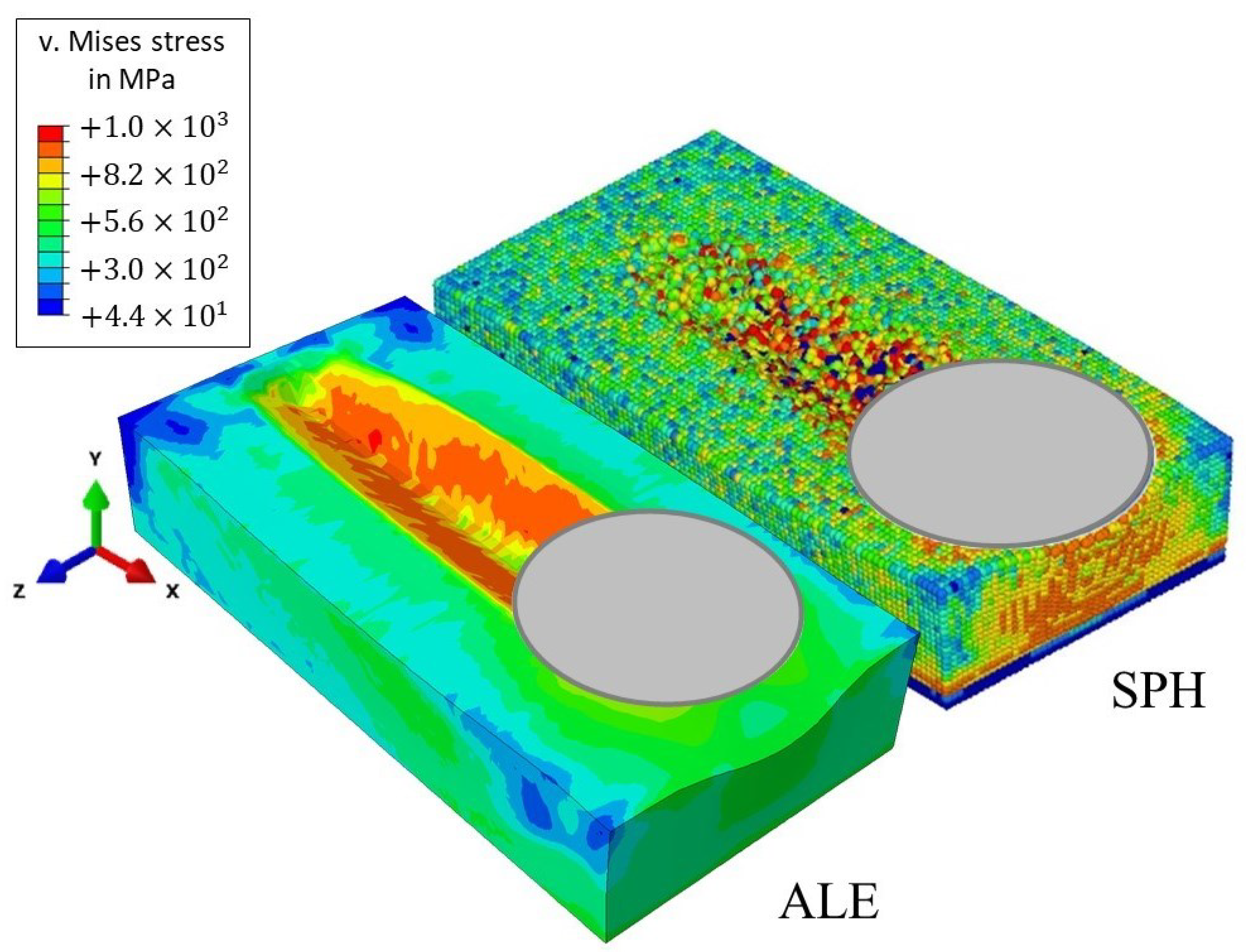
With the three discretization approaches (LAG, ALE, and SPH), 3D simulations of a single grit scratch were performed. Representative stress distribution of the ALE and SPH simulations are shown in Figure 12. The LAG model has a similar scratch profile to the ALE model. It can be observed that the von Mises stresses are highest for the elements along the path of the scratch and the stresses are more uniform for the ALE model than for the SPH model. The scratch topography is also better described by the ALE model, with a good demarcation of the groove and pile-up areas when compared to the SPH model.

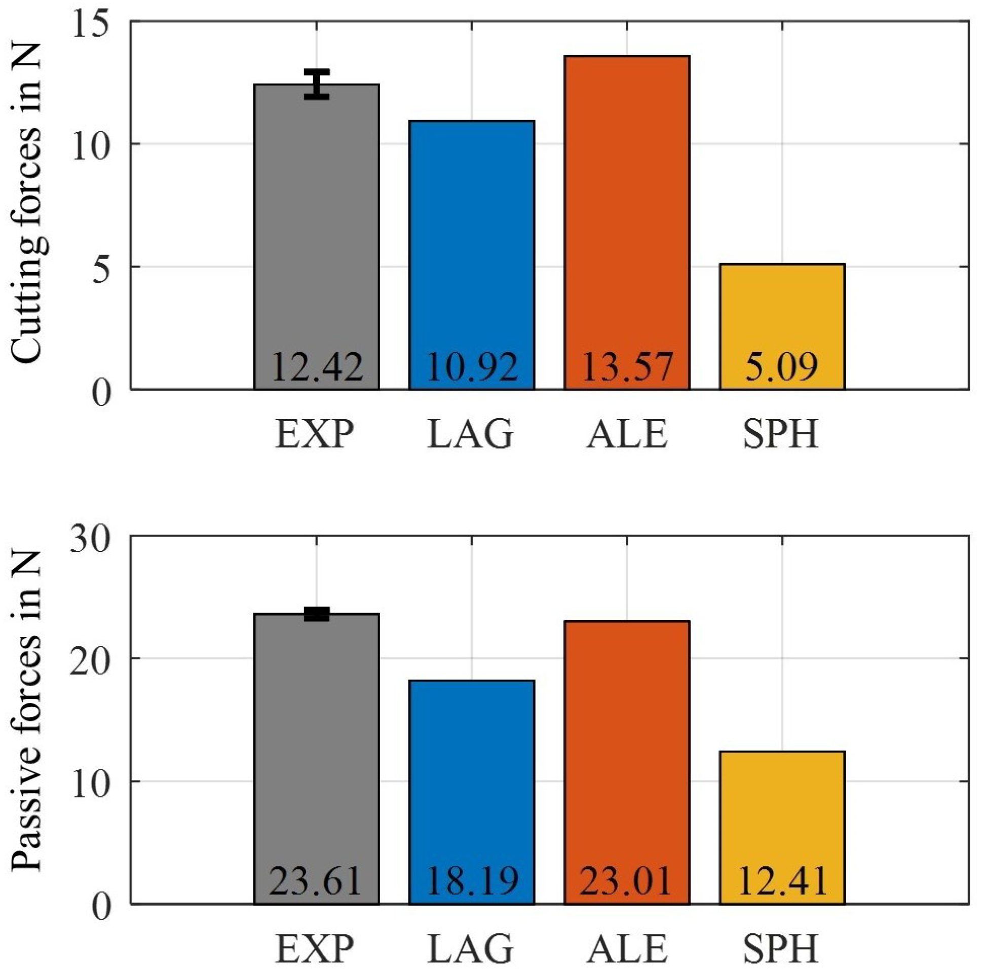
To verify the LAG, ALE, and SPH models, the process forces calculated by the 3D simulations are compared to the data obtained from the scratch experiments performed at our laboratory. Figure 13 shows the comparison of the experimental measurement of the process forces to the three discretizational approaches for a cutting speed of 200 mm/s and depth of cut of $a_p$ = 50 µm (corresponding to $a_{p,\mathrm{sim}}$ = 35 µm) and an indenter with cone angle of 105.

The average cutting force measured along the x-direction is 12.12 ± 0.8 N at steady state. The ALE model overestimates the cutting force with 13.57 N, whereas the LAG and SPH models underestimate the cutting force with 10.92 N and 5.09 N, respectively.

Similarly, the ALE model predicts the passive forces much better than the other discretization approaches. The average measured passive forces along the y-direction is 23.61 ± 0.32 N at steady state, which can be well reproduced with the ALE model and a value of 23.01 N. The other approaches again underestimate the passive forces, with 18.19 N (LAG) and 12.41 N (SPH).

Comparing details in the LAG and ALE approaches, both models have activated built-in element deletion algorithms. However, the elements in the LAG model do not employ a smoothing algorithm, which the ALE approach, by default, has. Hence, the elements in the LAG model are deleted prematurely, which leads to reduced process forces. In contrast, even though the SPH model does not employ any failure theory or element deletion technique, it underestimates the process forces as well. The error may be attributed to the cohesion model to connect particles. The SPH model does not consider the size effect (low depth of cuts), which is present in a micro-cutting process such as scratching [58,59]. Further additions may be necessary to the material model, and employment of a complex contact model can help alleviate the problem.

From the benchmark analysis, we can conclude that the ALE approach is best suited to model a scratch and the occurring forces. In the next section, we additionally show to what extent trends and dependencies on cutting speed and depth of cut can be mapped with the three discretization approaches.

5.3. Validation with Experiments

In this section, parameter studies are performed to compare the discretization approaches and their ability to represent measured trends in forces and changes in the workpiece topography. The process forces are investigated for five different cutting speeds ($v_c$ = 200–1000 mm/s) and two indenter geometries (cone angle = ${105}^{\circ }$ and ${120}^{\circ }$). Again, a reduced depth of cut $a_{p,\mathrm{sim}}$ = 35 µm was used in the simulation to represent the groove depth when scratching with a depth of cut $a_p$ = 50 µm during experiments. Additionally, for both indenter geometries, the resultant workpiece topographies of the ALE model are compared to measurements.

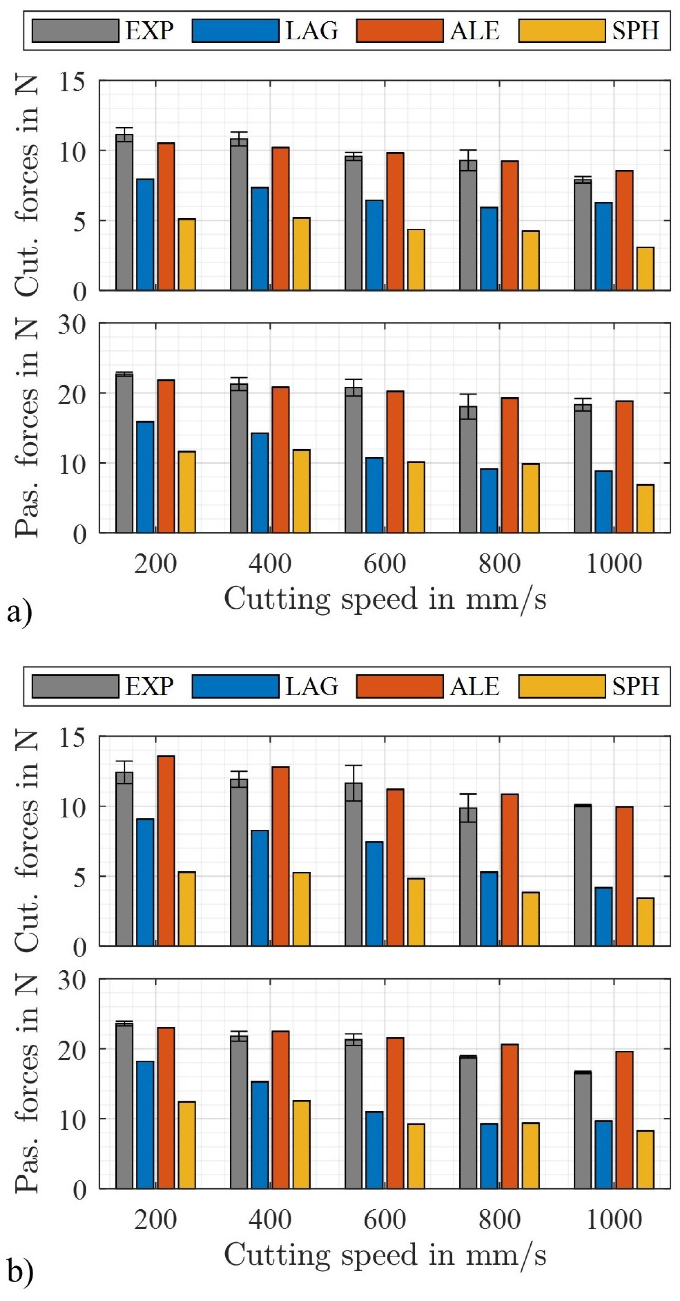
In Figure 14, the simulated averaged process forces are shown in comparison to the measurements. In addition, the values of the process forces and errors to the measurements for the cone angle $\gamma ={105}^{\circ }$ are shown in

Table 3. Comparison of measured cutting and passive force in a single grit scratch experiment with different numerical methods with an indenter cone angle of ${105}^{\circ }$. In the table, $F_c$ represents the experimental measured cutting force, $F_p$ represents the experimental measured passive force, $F_{c,\mathrm{sim}}$ represents the predicted cutting force, and $F_{p,\mathrm{sim}}$ represents the predicted passive force.

${\mathit{v}}_{\mathit{c}}$	Model	$\mathit{\gamma }$	${\mathit{F}}_{\mathit{c}}$	${\mathit{F}}_{\mathit{c},\mathbf{sim}}$	Error	${\mathit{F}}_{\mathit{p}}$	${\mathit{F}}_{\mathit{p},\mathbf{sim}}$	Error
mm/s		deg	N	N	%	N	N	%
200	LAG	105	11.12	7.92	28.77	22.68	15.88	29.98
200	ALE	105	11.12	10.51	5.49	22.68	21.88	3.53
200	SPH	105	11.12	5.09	54.21	22.68	11.59	48.90
400	LAG	105	10.81	7.32	32.28	21.27	14.25	33.00
400	ALE	105	10.81	10.20	5.64	21.27	20.80	2.21
400	SPH	105	10.81	5.19	52.04	21.27	11.84	44.33
600	LAG	105	9.571	6.44	32.77	20.75	10.63	48.77
600	ALE	105	9.571	9.83	2.65	20.75	20.20	2.65
600	SPH	105	9.571	4.36	54.45	20.75	10.11	51.30
800	LAG	105	9.28	5.93	36.08	18.04	9.13	49.41
800	ALE	105	9.28	9.23	0.59	18.04	19.25	6.71
800	SPH	105	9.28	4.24	54.28	18.04	9.86	45.35
1000	LAG	105	7.906	6.28	20.56	18.31	8.83	51.75
1000	ALE	105	7.906	8.55	8.10	18.31	18.80	2.68
1000	SPH	105	7.906	3.08	61.04	18.31	6.86	62.56

and for the cone angle $\gamma ={120}^{\circ }$ in

Table 4. Comparison of measured cutting and passive force in a single grit scratch experiment with different numerical methods with an indenter cone angle of ${120}^{\circ }$. In the table, $F_c$ represents the experimental measured cutting force, $F_p$ represents the experimental measured passive force, $F_{c,\mathrm{sim}}$ represents the predicted cutting force, and $F_{p,\mathrm{sim}}$ represents the predicted passive force.

${\mathit{v}}_{\mathit{c}}$	Model	$\mathit{\gamma }$	${\mathit{F}}_{\mathit{c}}$	${\mathit{F}}_{\mathit{c},\mathbf{sim}}$	Error	${\mathit{F}}_{\mathit{p}}$	${\mathit{F}}_{\mathit{p},\mathbf{sim}}$	Error
mm/s		deg	N	N	%	N	N	%
200	LAG	120	12.42	9.07	26.98	23.61	18.19	22.96
200	ALE	120	12.42	13.57	9.24	23.61	23.01	2.53
200	SPH	120	12.42	5.29	57.42	23.61	12.41	47.42
400	LAG	120	11.92	8.26	30.69	21.78	15.29	29.80
400	ALE	120	11.92	12.80	7.38	21.78	22.45	3.08
400	SPH	120	11.92	5.25	55.97	21.78	12.56	42.35
600	LAG	120	11.65	7.45	36.09	21.29	10.97	48.48
600	ALE	120	11.65	11.20	3.86	21.29	21.54	1.17
600	SPH	120	11.65	4.83	58.51	21.29	9.23	56.63
800	LAG	120	9.87	5.28	46.46	18.83	9.26	50.84
800	ALE	120	9.87	10.84	9.85	18.83	20.57	9.24
800	SPH	120	9.87	3.84	61.13	18.83	9.34	50.38
1000	LAG	120	10.05	4.17	58.46	16.62	9.65	41.97
1000	ALE	120	10.05	9.95	1.00	16.62	19.58	17.81
1000	SPH	120	10.05	3.43	65.85	16.62	8.27	50.25

. It is obvious that the ALE approach best represents the process forces. Nevertheless, all models correctly predict the tendency for process forces to decrease with increasing cutting speed. At high speeds, cutting is the predominant mechanism compared to rubbing and plowing [14], which leads to reduced process forces. In addition, when scratching at high cutting speeds, thermal softening is more significant than strain hardening, which leads to a further decrease in process forces. This tendency is also confirmed by experimental studies of [60,61].

Comparison of the results for the two cone angles (105^∘ and 120^∘) shows that the process forces increase with larger angle; compare with Figure 14a,b. This effect is especially visible at low cutting speeds of 200 mm/s and can be attributed to a larger contact length between tool and workpiece, which leads to higher compressive stresses, as already reported in [1,55,56]. All three discretization approaches reflect this tendency, although the ALE model is closest to the experimentally measured process forces. To further improve the results, optimization of strain rate sensitivity and thermal softening parameters in the Johnson–Cook model are recommended.

However, comparing the process forces between the discretization approaches and the experiments, we can see that the ALE approach is the most accurate, with an average error of 5.4% for the cutting forces and 5.2% for the passive forces (see Table 3 and Table 4), while the errors for the other numerical methods are over 30%.

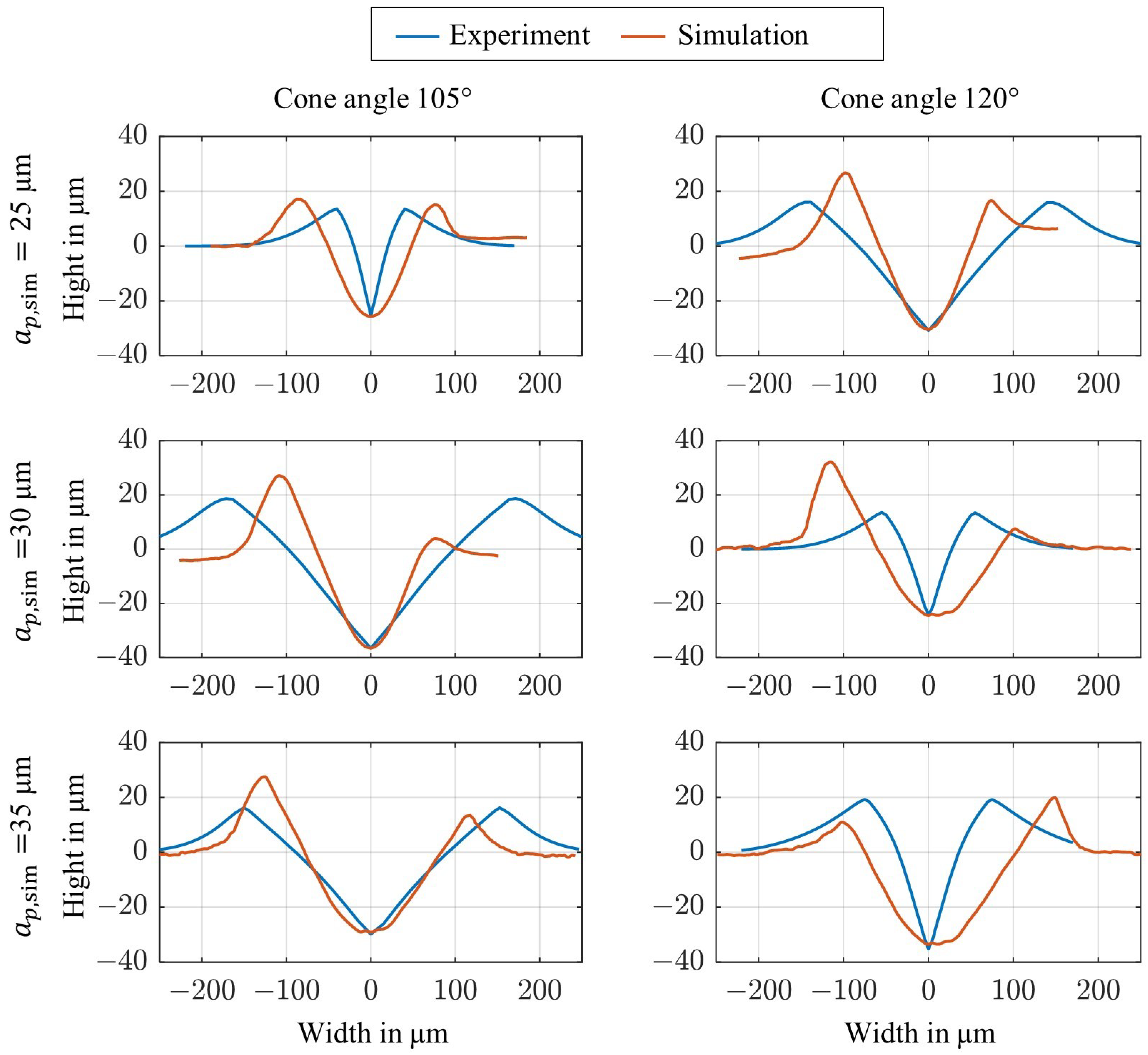
Therefore, we evaluated the surfaces of the scratches only for the ALE approach. Besides the evaluation of both indenter geometries, we also varied the depth of cut in the simulation $a_{p,\mathrm{sim}}$ about 25 µm, 30 µm, and 35 µm, which correspond to the three depths of cut in the experiments of $a_p=$ 40 µm, 45 µm, and 50 µm. Figure 15 shows the comparison of the 2D scratch topography between experiments and simulations. The ALE approach agrees well with the experimental results for all tested depths of cuts. It is observed that the model is quite robust in predicting both the groove area and the pile-up area. Thus, the ALE model is quite capable of predicting both the process forces and the scratch topography. This clearly proves that the ALE model is well suited to describe a single grain scratching process.

6. Conclusions

In this work, two numerical studies were conducted to evaluate the most appropriate discretization approach for a single grit scratching process and to determine if scratching can be represented by a simplified 2D model.

In the initial study, four discretizational approaches, LAG, ALE, SPH, and PFEM, were used for a 2D orthogonal cutting model. The models were initially benchmarked with a turning experiment for a positive orthogonal rake angle of $\gamma ={20}^{\circ }$. All of the discretizational approaches showed a good agreement with the experimental results in predicting the cutting forces, but had a high margin of error in predicting the passive forces. The 2D models were further extended to higher negative rake angles of $\gamma =0^{\circ }$ to $\gamma =-{60}^{\circ }$ to represent single grit scratching or grinding, respectively. In 2D, a total of 32 simulations were performed, resulting from four different numerical methods, eight different rake angles, and one cutting speed. Although the models qualitatively show an increase in the process forces with increase in negative rake angle, the simulation results do not match the experimental results of the scratch tests performed at our laboratory.

From the first study, we can conclude that due to the complex material removal mechanisms such as plowing, rubbing, and cutting, a single grit scratching process cannot be modeled in two dimensions.

To better capture these material removal mechanisms, a 3D benchmark model was developed for the three discretization approaches LAG, ALE, and SPH. With the 3D model, the trend that the passive forces are higher than the cutting forces was correctly reproduced. In general, the ALE model predicted the process forces much closer to the experimental results than the LAG and SPH models. Performing a parameter study using two indenters with cone angles of 105^∘ and 120^∘ for cutting speeds $v_c$ = 200–1000 mm/s revealed that the prediction of process forces by the ALE model best matches the experimental results and confirms the benchmark simulation results. A total of 50 scratch tests were performed with five repetitions for each cutting speed and cone angle, while 30 three-dimensional simulations were performed for the three different numerical models, five different speeds, and two different cone angles. The ALE approach showed the best correlation with experiments, with an average error of 5.4% for the cutting force and 5.2% for the passive force, while the other approaches showed errors above 30%. Furthermore, the ALE model was investigated based on the scratch topography with two indenter geometries for different depths of cut. It was shown that the ALE model is able to reliably predict both the groove and pile-up area.

In summary, we can conclude that the best discretization approach is the ALE formulation and that a 3D model is necessary because it not only predicts the process forces close to the experimentally measured values, but also is able to represent the trends observed when performing the individual scratch experiments and scratch topography.

The research carried out in this article opens up new lines of research in both numerical modeling and experimental design. In terms of numerical modeling, new techniques for solving the differential equations describing mechanical and thermal phenomena can be applied to grinding models. Among them, we find the particle finite element method [30,62,63], the material point method [64,65], the element-free Galerking [66], and stabilized optimal transportation mesh-free (OTM) method [67,68,69]. These techniques have been successfully applied to 2D orthogonal cutting simulation; however, the application to 3D simulation of grinding is a field of research to be explored, since there is no available literature, and the numerical methods mentioned are not implemented in commercial software yet.

In addition, the constitutive model used can be improved with models based on physics, for example, models based on dislocations [70,71,72]. These models have been successfully applied to the numerical simulation of orthogonal cutting [70,71,72], showing a better prediction of cutting and feed forces.

At the same time, in a large number of numerical orthogonal cutting investigations, it has been identified that the difference between numerical models and experimental tests is due to the use of Coulomb’s law of friction. For this reason, the use of friction values depending on temperature [73], or relative sliding velocity between chip and tool [73], among other friction models [54,74,75,76], has been proposed. We expect future research to study the influence of friction models in the simulation of the grinding process.

Still, using the same numerical models discussed in the present work, the grinding process can be investigated with different indenter geometries, at different cutting speeds, at different depths of cut, with new workpiece and tool materials, and including the effect of the coolant to further enhance the existing models for a closer match with experiments.