Article

Top Surface Roughness Modeling for Robotic Wire Arc Additive Manufacturing

1
Ingram School of Engineering, Texas State University, San Marcos, TX 78666, USA
2
Department of Electrical and Computer Engineering, University of Kentucky, Lexington, KY 40506, USA
*
Author to whom correspondence should be addressed.
J. Manuf. Mater. Process. 2022, 6(2), 39; https://doi.org/10.3390/jmmp6020039
Submission received: 2 February 2022 / Revised: 8 March 2022 / Accepted: 17 March 2022 / Published: 21 March 2022
(This article belongs to the Special Issue Machine Intelligence in Welding and Additive Manufacturing)

Abstract

:
Wire Arc Additive Manufacturing (WAAM) has many applications in fabricating complex metal parts. However, controlling surface roughness is very challenging in WAAM processes. Typically, machining methods are applied to reduce the surface roughness after a part is fabricated, which is costly and ineffective. Therefore, controlling the WAAM process parameters to achieve better surface roughness is important. This paper proposes a machine learning method based on Gaussian Process Regression to construct a model between the WAAM process parameters and top surface roughness. In order to measure the top surface roughness of a manufactured part, a 3D laser measurement system is developed. The experimental datasets are collected and then divided into training and testing datasets. A top surface roughness model is then constructed using the training datasets and verified using the testing datasets. Experimental results demonstrate that the proposed method achieves less than 50 μm accuracy in surface roughness prediction.

1. Introduction

Wire Arc Additive Manufacturing (WAAM) is an additive manufacturing process for fabricating metal parts which has been used in many production processes in industries such as automotive, aerospace, nuclear, oil and gas, shipbuilding, and heavy equipment manufacturing [1,2,3]. Controlling the surface roughness of the manufactured parts is one of the challenging problems in WAAM processes. The surface roughness evaluation can be categorized into the top surface roughness evaluation [4,5] and side surface roughness evaluation [6,7]. Both are important for WAAM because the roughness will affect the properties of the final product. Yehorov et al. [7] evaluated the side surface waviness of thin walls produced by varying the current, wire feed speed, and travel speed. The experimental results show that a suitable range of travel speed can mitigate the roughness of the produced surfaces. Li et al. [8] developed a WAAM process to manufacture a thin-walled structure. The side surface roughness is about 5 μm, which is much better than that of other research methods. However, the proposed technique used small-power metal fine wire feeding, which is not feasible for most additive manufacturing applications when manufacturing large parts.
The top surface roughness or waviness is also worth investigating [1,4]. As we know, the top surface roughness is affected by the deposition pattern and welding process parameters. In order to improve the fabrication efficiency and accuracy, industrial robots have been widely used in the WAAM processes [9]. Various robot path planning methods such as weaving, zigzag, raster, and Medial Axis Transformation have been used in WAAM [10]. Using these different path patterns, the roughness of the produced layers is different. Typically, machining is needed to reduce the surface roughness [1,4]. Most researchers model the weld bead using a parabolic function for a straight path [4,11] and reasonable results are achieved. Aldalur etc. [12] compared the performance of an overlapping path with that of a weaving path and they found that the weaving path achieved better surface roughness; they also mentioned that similar mechanical properties including tensile strength, hardness and Charpy were obtained. Therefore, we will investigate the surface roughness for WAAM using a robotic weaving path. Besides the robot welding path, WAAM process parameters will also affect the surface roughness [4]. In order to reduce the machining cost and improve WAAM efficiency and properties of the final product, the top surface roughness must be minimized during the WAAM processes. Thus, robot path parameters and WAAM process parameters should be investigated in order to minimize the surface roughness.
In order to control the surface roughness, a model which establishes a relationship between the robotic WAAM parameters (path and process parameters), and top surface roughness must be constructed.
The Response Surface Methods have been implemented in the top surface roughness modeling [13,14]. However, it is difficult for these methods to accurately model the complex welding process to predict the surface roughness because only polynomial fittings are used. Recently machine learning methods have been implemented to model top surface roughness. Different machine learning methods have been proposed [4,15,16]. Xia et al. [16] explored surface roughness modeling and prediction methods based on Adaptive Neuro-fuzzy Inference System (ANFIS), Extreme Learning Machine and Support Vector Regression. They compared the performances of these methods and found that ANFIS achieved better results in terms of mean absolute percentage error (MAPE) which is about 14.15%. Yaseer et al. [5] proposed a machine learning method based on Random Forest to model the surface roughness. Their results show that the MAPE is 5.64%. Even though this method achieves better MAPE, the computation is quite complex. Therefore, more investigation about predicting the top surface roughness with high accuracy is needed, especially for robotic WAAM processes using a weaving path.
Machine learning methods based on Gaussian Process Regression (GPR) have been widely used to model some very complex processes in different applications [17,18,19,20]. These methods can deal with system uncertainties and noisy observations in complex system modeling [21]. Therefore, it is desirable to develop a modeling method based on GPR for complex WAAM roughness modeling.
In this paper, we propose a machine learning method based on GPR to establish a relationship between the robotic WAAM parameters and produced surface roughness using a weaving path. The procedures to collect training and testing datasets are detailed. A surface roughness measurement method is presented. After the model based on GPR is constructed, the testing datasets are used to test the accuracy of the generated model. The experimental results are presented, and analysis is detailed. The results demonstrate that the proposed machine learning method based on GPR achieves about 50 μ m accuracy in WAAM surface roughness modeling. The main contributions of this paper are:
  • A machine learning method based on GPR is developed to model the top surface roughness for robotic weaving path;
  • The proposed method is tested experimentally, and the results demonstrate that about 50 μ m accuracy of the top surface roughness is achieved.

2. Materials and Methods

WAAM is a very complex process and it is difficult to predict the surface roughness. Therefore, a method based on GPR is proposed to establish the relationship between the robotic WAAM parameters and surface roughness. An industrial robot is programmed to perform the WAAM process using a weaving path. A 3D measurement system is used to collect the surface dimensional data. Using the collected datasets, a model based on GPR is then constructed.

2.1. Robotic WAAM Process

For robotic WAAM processes, there are two major problems: robot trajectory planning and WAAM process parameter control. Different methods have been developed for robotic WAAM path generation such as raster, grid, zigzag, contour offset, spiral, and weaving [22,23,24]. In this paper, we will study the roughness for robotic WAAM process using a weaving path as shown in Figure 1.
As we can see in Figure 1, there are three parameters to be determined: travel speed, weaving wavelength, and weaving amplitude. These parameters will affect the surface roughness. The WAAM process parameters include wire feed speed, welding current, welding voltage, wire electrode size, type of shielding gas, electrode extension and electrode angle, etc. [25]. In this paper, only four parameters are considered: wire feed speed F S , travel speed ( T S ), weaving wavelength ( W W ), and weaving amplitude ( W A ). Other parameters are fixed in the experiments.

2.2. Data Collection and Roughness Measurement

For a robotic WAAM process, the input parameters can be defined as:
θ = [ F S T S W W W A ]
where θ  is a vector of the robotic WAAM parameters. The surface roughness R can be modeled using the input parameters as:
R = ρ ( θ ) + ν
where ν N 0 , σ is Gaussian noise with mean 0 and variance σ . ρ ( θ ) is a Gaussian Process. Constructing a physical model for a robotic WAAM process to predict the roughness is almost impossible because the complexity of the system which a includes robotic system and a welding system, etc. However, we can collect experimental data to construct a model using machine learning methods. By performing experiments, we can obtain the experimental data ( θ , R ) in Equations (1) and (2). The input vector θ can be set before experiments and recorded. After an experiment is performed, a part can be fabricated. A fabricated part surface is shown in Figure 2.
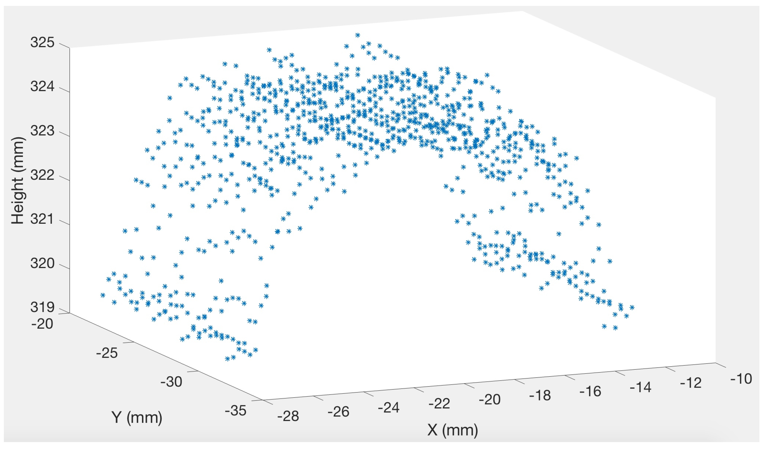
In order to measure the surface roughness shown in Figure 2, a 3D laser scanning system is used. After the surface is scanned, point cloud data can be collected. The collected point cloud data must be processed in order to obtain the top surface roughness. Because the 3D laser scanning system measures a larger area than the top surface area of a fabricated part, the extra point cloud data must be removed. In order to explain the method we developed to obtain the top surface roughness, we use an example of the collected point cloud data of a fabricated part surface as shown in Figure 3.
In order to remove the extra data points, we fit several planes to the point cloud data. Because the top surface roughness is computed using data points on the top surface, the edge data in the point cloud should be removed first. We fit a plane to the point cloud data and remove all data points below the plane. Using the data points above the plane, another plane is fitted again and the data points below the plane are removed again. The process continues until all edge data points are removed. Using all data points above the final plane, a final plane is fitted to find the top surface roughness. Suppose the fitted plane is:
a x + b y + c z + 1 = 0
where a , b , c are coefficients and x , y , z are coordinates. The roughness is then calculated using the following equation:
R = 1 K k = 1 K | a x k + b y k + c z k + 1 | a 2 + b 2 + c 2
where K is the total number of points used to calculate the roughness; ( x k , y k , z k ) are the coordinates of the k t h  point.
After n experiments are performed, n sets of experimental data ( θ , R ) can be obtained. These n datasets can be used as training datasets:
θ = [ θ 1 , θ 2 , . . . , θ n ] R = [ R 1 , R 2 , . . . , R n ]

2.3. Modeling Method

Once the experimental datasets are obtained, we can construct a model between the input parameters and output surface roughness. GPR is a machine learning method which has been used to construct a model for a complex process in many applications. In Equation (2), ρ ( θ ) is defined using mean and covariance function:
ρ ( θ ) GP ( m ( θ ) , k ( θ , θ ) )
where GP represents the Gaussian Process; θ is a set of arbitrary input WAAM parameters; m ( θ ) and k ( θ , θ ) are mean and covariance function, respectively.
The covariance function k θ , θ is defined as:
k θ , θ = E [ ( m ( θ ) R ( θ ) ) ( m ( θ ) R ( θ ) ) ]
Different covariance functions can be used for model construction as shown in Table 1.
The covariance functions have hyperparameters which should be determined in order to construct a model. For example, the Gaussian Radial Basis function has one hyperparameter β . Because different covariance function may have different number of hyperparameters, we denote the hyperparameters using vector h .
The covariance functions can also be combined to generate a new covariance function for model construction; for example,
k ( θ , θ ) = p = 1 P w p k p ( θ , θ )
where k p ( θ , θ ) is the p t h covariance function and w p is its weight. For the combined covariance function, more hyperparameters should be determined.
For a training dataset ( θ , R ) , the posterior probability of ρ ( θ ) can be calculated:
p ρ θ , R , h = p R θ , ρ , h p ρ θ , h p R θ , h
We can then compute the marginal likelihood:
p R θ , h = p R θ , ρ , h p ρ θ , h d ρ
As we can see that p R θ , h is the likelihood of hyperparameters h . The log marginal likelihood can then be derived:
log p R θ , h = 1 2 R T Γ 1 R 1 2 log Γ n 2 log 2 π
where Γ is defined as:
Γ = K θ , θ + σ 2 I
The hyperparameters can then be optimized by maximizing the log marginal likelihood:
h * = argmax h log p R θ , h
After the optimal hyperparameters are obtained, the covariance function can be determined, and a roughness prediction model can be established. For a given set of input parameters θ * , the output roughness R * can be predicted. For m sets of given input parameters
θ * = [ θ 1 * , θ 2 * , . . . , θ m * ] ,
let the predicted output parameters be
R * = [ R 1 * , R 2 * , . . . , R m * ] .
The joint marginal likelihood of output parameters can be expressed as:
p ( R , R * ) N 0 , K
where
K = K θ , θ + σ 2 I K θ , θ * K θ * , θ K θ * , θ *
where K ( θ , θ ) ( θ and θ represent θ and θ * ) is a matrix defined using covariance function k ( θ i , θ j ) :
K i j ( θ , θ ) = k ( θ i , θ j )
where K i j ( θ , θ ) is the element in the matrix K ( θ , θ ) .
We can then calculate the output surface roughness R * using the conditional distribution:
p ( R * θ , R , θ * ) N μ ( R * ) , V R *
μ ( R * ) = K θ * , θ Γ 1 R V R * = K θ * , θ * K θ * , θ Γ 1 K θ , θ *
where μ ( R * ) and V R * are the predicted mean and variance of R * , respectively. Therefore, given a set of input parameters θ * , the mean and variance of the output surface roughness R * can be predicted.

3. Results and Discussions

To validate the proposed modeling method using GPR, a WAAM system and a measurement system were developed.
Figure 4 shows the developed WAAM system which includes an ABB IRB140 robot with IRC5 controller, a welding machine (Thermal Arc PowerMaster 500 by Thermadyne Industries, Inc., West Lebanon, NH, USA), a Miller r-115 wire feeder and a shielding gas tank.
The flow rate of the shielding gas (90% Argon and 10% CO2) was 31.78 f t 3 /h, and 1.2 mm diameter steel wire (ER70S-6) was used. Direct current reverse polarity (DCRP) was used for connecting the welding machine with the MIG gun and substrate.
Thirty trial experiments were performed using different robotic WAAM process parameters, and we found that the bead cross-section tends to be parabolic instead of flat with the increase in travel speed and wire feed speed using a weaving path. Higher wire feed speed causes more spatter. Considering these issues, we chose the values of input parameters as shown in Table 2 to perform the experiments.
As we can see from Table 2, there were four input parameters. The ABB robot was programmed to perform the experiments. We totally fabricated 45 parts. Figure 5 shows some examples of the fabricated parts.
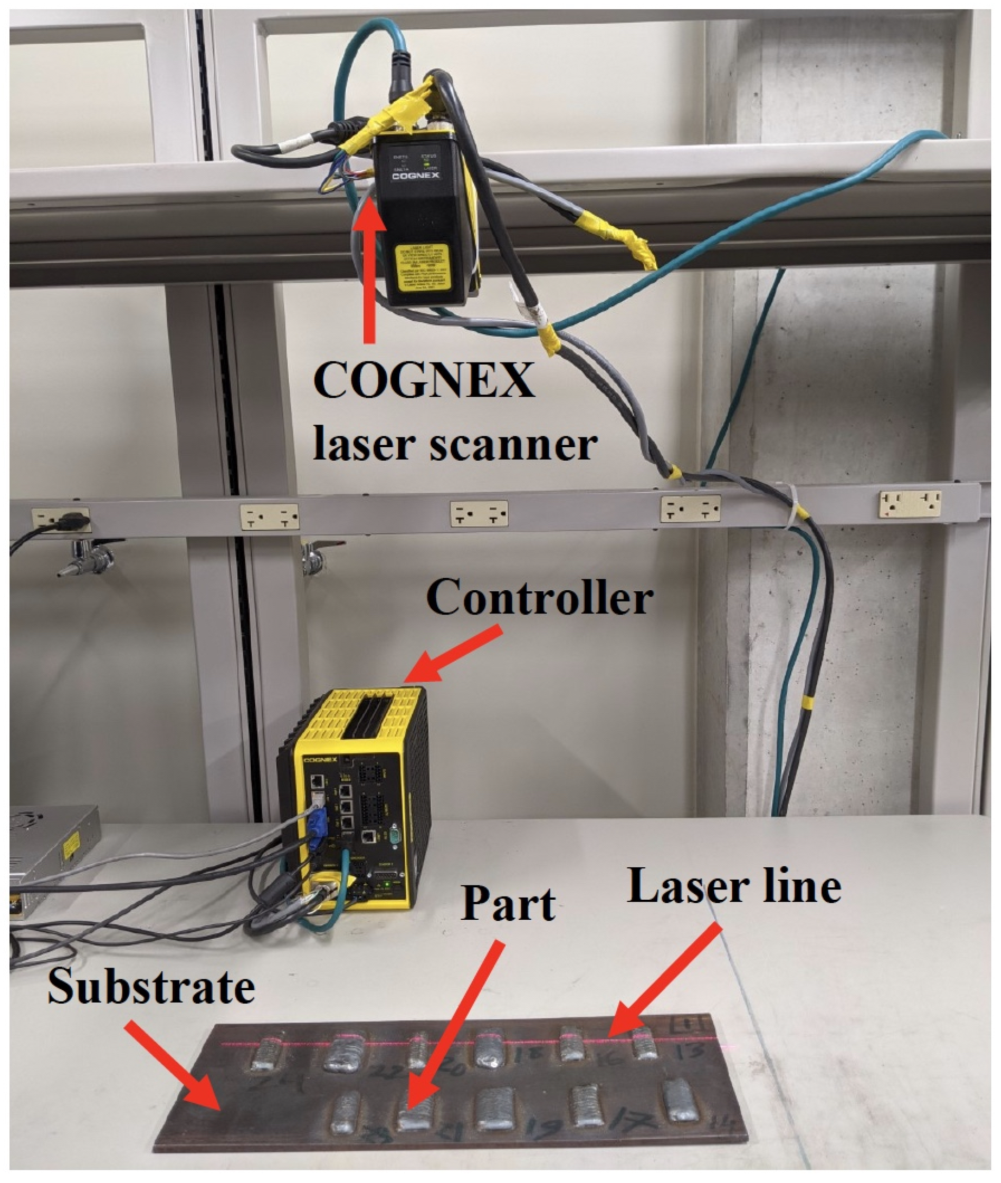
In order to measure the surface roughness of the fabricated parts, a measurement system is developed and shown in Figure 6.
The measurement system includes a Cognex 3D laser scanner with measurement accuracy 10 μ m. After scanning the manufactured part, point cloud data can be obtained. We processed the data using MATLAB by fitting a series of planes. In this research, we found that fitting two planes was good enough to compute the surface roughness. Figure 7 shows the results after fitting the first plane and the second plane. The data above the first fitted plane were used to calculate the surface roughness.
For the 45 parts, we collected the point cloud data and computed the surface roughness. We obtained a total of 45 datasets. Figure 8 shows one example of the relationship between the robotic WAAM parameters ( T s and F s ) and the surface roughness. From the figure, we can see that their relationship is quite nonlinear.
The learning method based on GPR was then implemented to construct a model to establish the relationship between the robotic WAAM process parameters and the top surface roughness. In the training process, we combined three covariance functions to generate a covariance function for model construction: noise, Squared Exponential Function and Gaussian Radial Basis Function. Therefore, there were four hyperparameters to be optimized. The weight w p for the three covariance functions was set to be 1.
We divided the recorded 45 datasets into 40 training datasets and 5 testing datasets randomly. We constructed a model using the training datasets based on the proposed GPR method. We then used the five testing datasets to test the model. The software flowchart is shown in Algorithm 1.
Algorithm 1: Model Construction and Testing Procedures Based on GPR.
procedure
    Read experimental datasets from a file
    Randomly divide the datasets into 40 training datasets and 5 testing datasets
    Construct a model based on GPR using the training datasets
    loop the 40 training datasets:
    Input the robotic WAAM process parameters in the training dataset into the constructed model and obtain the predicted top surface roughness
    Compute RMS error using the predicted top surface roughness and the actual top surface roughness
    Record the maximum top surface roughness
    goto loop.
    loop the 5 testing datasets:
    Input the robotic WAAM process parameters in the testing dataset into the constructed model and obtain the predicted top surface roughness
    Compute the RMS error using the predicted top surface roughness and the actual top surface roughness
    Record the maximum top surface roughness
    goto loop.
    close
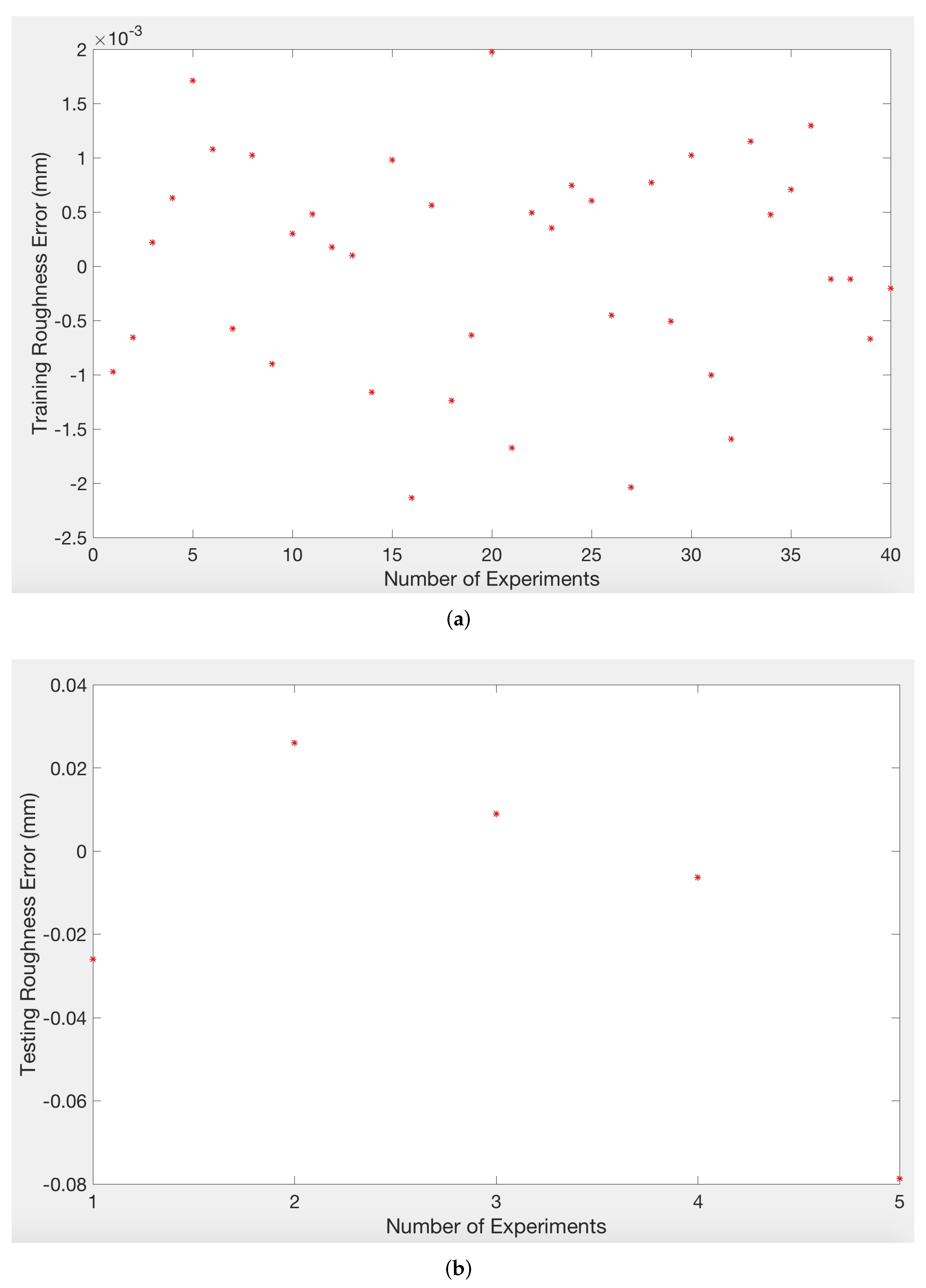
Figure 9a shows one of the results of training errors of the 40 training datasets and Figure 9b one of the results of the five testing datasets.
This model construction and testing process was performed about 100 times using the randomly generated training and testing datasets and the results were recorded. Table 3 summarizes the maximum errors and root mean square (RMS) errors of the training datasets and testing datasets in four trials.
As we can see in Table 3, the maximum error of the training datasets is less than 2.5 μ m and the RMS error is less than 1 μ m. The results mean that the modeling accuracy is very high using the training datasets. In order to demonstrate the modeling accuracy, we also used the random testing datasets to validate the model. Table 3 shows the maximum prediction error is less than 50 μ m and the RMS error is less than 30 μ m. The testing results demonstrate that the modeling method using GPR can accurately predict the surface roughness given a set of robotic WAAM parameters.

4. Conclusions and Future Work

One of the challenges in the WAAM process is to control the surface roughness, which is affected by the WAAM process parameters. A machine learning method based on Gaussian Process Regression was developed to model the relationship between the WAAM process parameters and top surface roughness. Experiments were performed and the surface roughness was measured using a 3D laser scanning system. After the datasets were collected, they were divided into the training and testing datasets. A model was then generated using the training datasets and tested using the testing datasets. The experimental results show that the maximum prediction error was less than 50 μ m, which demonstrates the effectiveness of the modeling method using Gaussian Process Regression. Our future work will focus on modeling the surface height and surface width together with the top surface roughness. Once the model is created, we can explore an optimal set of WAAM process parameters such that desired surface height, surface width, and minimal top surface roughness can be achieved, which is useful for variable layer thickness and printing width in additive manufacturing.

Author Contributions

Conceptualization, H.C.; methodology, H.C.; software, H.C. and A.Y.; validation, A.Y. and H.C.; formal analysis, H.C. and A.Y.; investigation, H.C.; resources, H.C. and Y.Z.; data curation, A.Y. and H.C.; writing—original draft preparation, H.C.; writing—review and editing, H.C.; visualization, H.C. and A.Y.; supervision, H.C. and Y.Z.; project administration, H.C.; funding acquisition, H.C. and Y.Z. All authors have read and agreed to the published version of the manuscript.

Funding

The research is partially supported by the Research Enhancement Program, Texas State University.

Data Availability Statement

Not applicable.

Conflicts of Interest

The authors declare no conflict of interest.

References

  1. Chaturvedi, M.; Scutelnicu, E.; Rusu, C.C.; Mistodie, L.R.; Mihailescu, D.; Subbiah, A.V. Wire Arc Additive Manufacturing: Review on Recent Findings and Challenges in Industrial Applications and Materials Characterization. Metals 2021, 11, 939. [Google Scholar] [CrossRef]
  2. Li, Y.; Su, C.; Zhu, J. Comprehensive review of wire arc additive manufacturing: Hardware system, physical process, monitoring, property characterization, application and future prospects. Results Eng. 2022, 13, 100330. [Google Scholar] [CrossRef]
  3. Popov, V.V.; Fleisher, A. Hybrid additive manufacturing of steels and alloys. Manuf. Rev. 2020, 7, 6. [Google Scholar] [CrossRef] [Green Version]
  4. Ding, D.; He, F.; Yuan, L.; Pan, Z.; Wang, L.; Ros, M. The first step towards intelligent wire arc additive manufacturing: An automatic bead modelling system using machine learning through industrial information integration. J. Ind. Inf. Integr. 2021, 23, 100218. [Google Scholar] [CrossRef]
  5. Yaseer, A.; Chen, H. Machine learning based layer roughness modeling in robotic additive manufacturing. J. Manuf. Process. 2021, 70, 543–552. [Google Scholar] [CrossRef]
  6. Dordlofva, C.; Torlind, P. Evaluating design uncertainties in additive manufacturing using design artefacts: Examples from space industry. Des. Sci. 2020, 6, e12. [Google Scholar] [CrossRef]
  7. Yehorov, Y.; da Silva, L.J.; Scotti, A. Balancing WAAM Production Costs and Wall Surface Quality through Parameter Selection: A Case Study of an Al-Mg5 Alloy Multilayer-Non-Oscillated Single Pass Wall. J. Manuf. Mater. Process. 2019, 3, 32. [Google Scholar] [CrossRef] [Green Version]
  8. Li, B.; Wang, B.; Zhu, G.; Zhang, L.; Lu, B. Low-Roughness-Surface Additive Manufacturing of Metal-Wire Feeding with Small Power. Materials 2021, 14, 4265. [Google Scholar] [CrossRef]
  9. Urhal, P.; Weightman, A.; Diver, C.; Bartolo, P. Robot assisted additive manufacturing: A review. Robot. Comput.-Integr. Manuf. 2019, 59, 335–345. [Google Scholar] [CrossRef]
  10. Yaseer, A.; Chen, H. A Review of Path Planning for Wire Arc Additive Manufacturing (WAAM). J. Adv. Manuf. Syst. 2021, 20, 589–609. [Google Scholar] [CrossRef]
  11. Suryakumar, S.; Karunakaran, K.; Bernard, A.; Chandrasekhar, U.; Raghavender, N.; Sharma, D. Weld bead modeling and process optimization in Hybrid Layered Manufacturing. Comput.-Aided Des. 2011, 43, 331–344. [Google Scholar] [CrossRef]
  12. Aldalur, E.; Veiga, F.; Suarez, A.; Bilbao, J.; Lamikiz, A. Analysis of the Wall Geometry with Different Strategies for High Deposition Wire Arc Additive Manufacturing of Mild Steel. Metals 2020, 10, 892. [Google Scholar] [CrossRef]
  13. Deng, Y.; Mao, Z.; Yang, N.; Niu, X.; Lu, X. Collaborative Optimization of Density and Surface Roughness of 316L Stainless Steel in Selective Laser Melting. Materials 2020, 13, 1601. [Google Scholar] [CrossRef] [PubMed] [Green Version]
  14. Tian, H.; Lu, Z.; Li, F.; Chen, S. Predictive Modeling of Surface Roughness Based on Response Surface Methodology after WAAM. In Proceedings of the International Conference on Electronical, Mechanical and Materials Engineering (ICE2ME 2019), Wuhan, China, 20–21 January 2019. [Google Scholar] [CrossRef] [Green Version]
  15. Charles, A.; Elkaseer, A.; Thijs, L.; Hagenmeyer, V.; Scholz, S. Effect of Process Parameters on the Generated Surface Roughness of Down-Facing Surfaces in Selective Laser Melting. Appl. Sci. 2019, 9, 1256. [Google Scholar] [CrossRef] [Green Version]
  16. Xia, C.; Pan, Z.; Polden, J.; Li, H.; Xu, Y.; Chen, S. Modelling and prediction of surface roughness in wire arc additive manufacturing using machine learning. J. Intell. Manuf. 2021, 1–16. [Google Scholar] [CrossRef]
  17. Vasudevan, S.; Ramos, F.; Nettleton, E.; Durrant-Whyte, H. Gaussian process modeling of large-scale terrain. J. Field Robot. 2009, 26, 812–840. [Google Scholar] [CrossRef]
  18. Frank, B.; Stachniss, C.; Abdo, N.; Burgard, W. Using Gaussian Process Regression for Efficient Motion Planning in Environments with Deformable Objects. In Proceedings of the Twenty-Fifth AAAI Conference on Artificial Intelligence, San Francisco, CA, USA, 7–8 August 2011. [Google Scholar]
  19. Schneider, M.; Ertel, W. Robot Learning by Demonstration with local Gaussian process regression. In Proceedings of the 2010 IEEE/RSJ International Conference on Intelligent Robots and Systems, Taipei, Taiwan, 18–22 October 2010; pp. 255–260. [Google Scholar]
  20. Jadaliha, M.; Xu, Y.; Choi, J.; Johnson, N.; Li, W. Gaussian Process Regression for Sensor Networks Under Localization Uncertainty. Signal Process. IEEE Trans. 2013, 61, 223–237. [Google Scholar] [CrossRef]
  21. Grancharova, A.; Kocijan, J.; Johansen, T.A. Explicit stochastic predictive control of combustion plants based on Gaussian process models. Automatica 2008, 44, 1621–1631. [Google Scholar] [CrossRef] [Green Version]
  22. Jiang, J.; Ma, Y. Path Planning Strategies to Optimize Accuracy, Quality, Build Time and Material Use in Additive Manufacturing: A Review. Micromachines 2020, 11, 633. [Google Scholar] [CrossRef]
  23. Ma, G.; Zhao, G.; Li, Z.; Xiao, W. A Path Planning Method for Robotic Wire and Arc Additive Manufacturing of Thin-Walled Structures with Varying Thickness. IOP Conf. Ser. Mater. Sci. Eng. 2019, 470, 012018. [Google Scholar] [CrossRef]
  24. Ding, D.; Pan, Z.; Cuiuri, D.; Li, H. Process Planning Strategy for Wire and Arc Additive Manufacturing. In Robotic Welding, Intelligence and Automation. RWIA 2014. Advances in Intelligent Systems and Computing; Springer: Cham, Switzerland, 2014; Volume 363. [Google Scholar]
  25. Chen, H.; Zhang, B.; Fuhlbrigge, T. Welding Process Optimization Methods: A Review. Trans. Intell. Weld. Manuf. 2020, 3–21. [Google Scholar] [CrossRef]
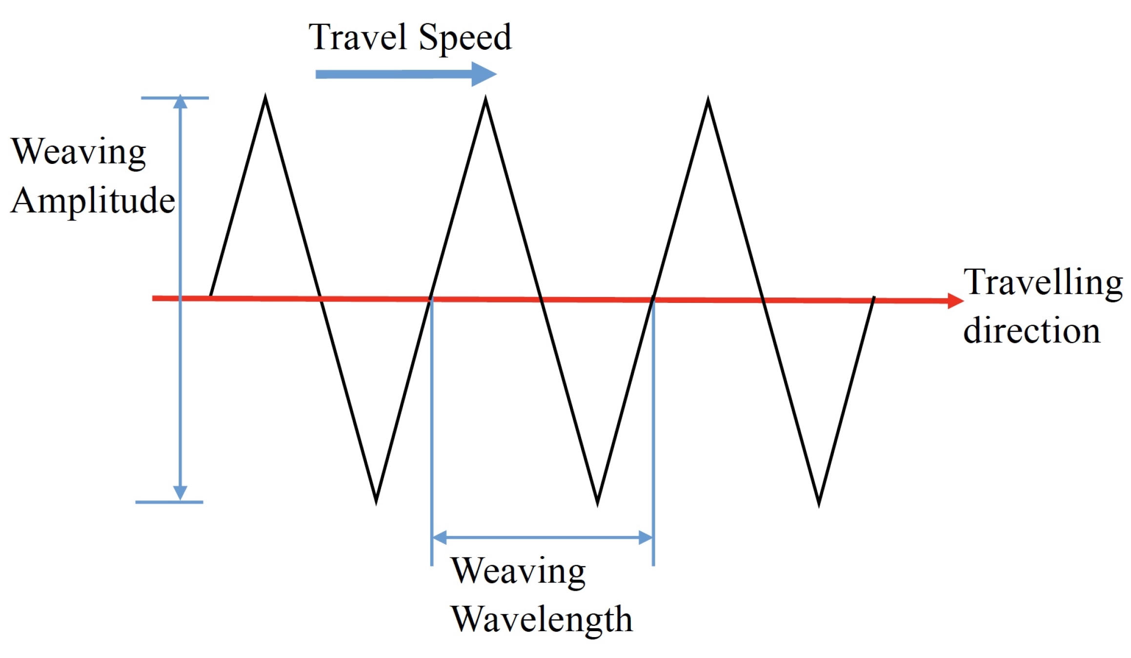
Figure 1. A robotic weaving path. There are three trajectory parameters: travel speed, weaving wavelength, and weaving amplitude.
Jmmp 06 00039 g001
Figure 2. A fabricated part on a substrate.
Jmmp 06 00039 g002
Figure 3. One example of the measured point cloud data of a fabricated part. The height is measured relative to the frame of the 3D laser scanning system. * in the figure represents data points.
Jmmp 06 00039 g003
Figure 4. The developed experimental system.
Jmmp 06 00039 g004
Figure 5. The fabricated parts using different parameters.
Jmmp 06 00039 g005aJmmp 06 00039 g005b
Figure 6. The developed measurement system for surface roughness.
Jmmp 06 00039 g006
Figure 7. Fitted planes to the point cloud data to obtain surface roughness. The points below the plane will be removed and the points above the plane are used to fit the next plane. • represents data points.
Jmmp 06 00039 g007
Figure 8. The relationship between the robotic WAAM parameters and surface roughness. * represents data points.
Jmmp 06 00039 g008
Figure 9. The errors of the training datasets and testing datasets: (a) errors of the 50 training datasets; (b) errors of the 5 testing datasets. * represents data points.
Jmmp 06 00039 g009
Table 1. Covariance functions k ( θ , θ ) .
NameEquation
Noise Function σ 2
Linear Function θ · θ
Squared Exponential Function σ 2 exp | θ θ | 2 2 l 2
Gaussian Radial Basis Function exp ( β θ θ 2 )
Sigmoid Function tanh β ( θ · θ ) + c
Polynomial Function β ( θ · θ ) + c α
Note: σ, l, β, c and α are hyperparameters.
Table 2. The range of the input parameters used in experiments.
Input ParametersMinimum ValuesMaximum Values
F S (inches/minute)6090
T S (mm/s)35
W W (mm)24
W A (mm)612
Table 3. The Testing Results.
TrialRMS1 ( μ m)Max1 ( μ m)RMS2 ( μ m)Max2 ( μ m)
10.0640.17822.83041.001
20.0960.26927.10245.626
30.8342.15322.23834.499
40.0650.14928.40746.845
Note: Max1 and RMS1 are the maximum error and RMS error of the training datasets, respectively; Max2 and RMS2 are the maximum error and RMS error of the testing datasets, respectively.
Publisher’s Note: MDPI stays neutral with regard to jurisdictional claims in published maps and institutional affiliations.