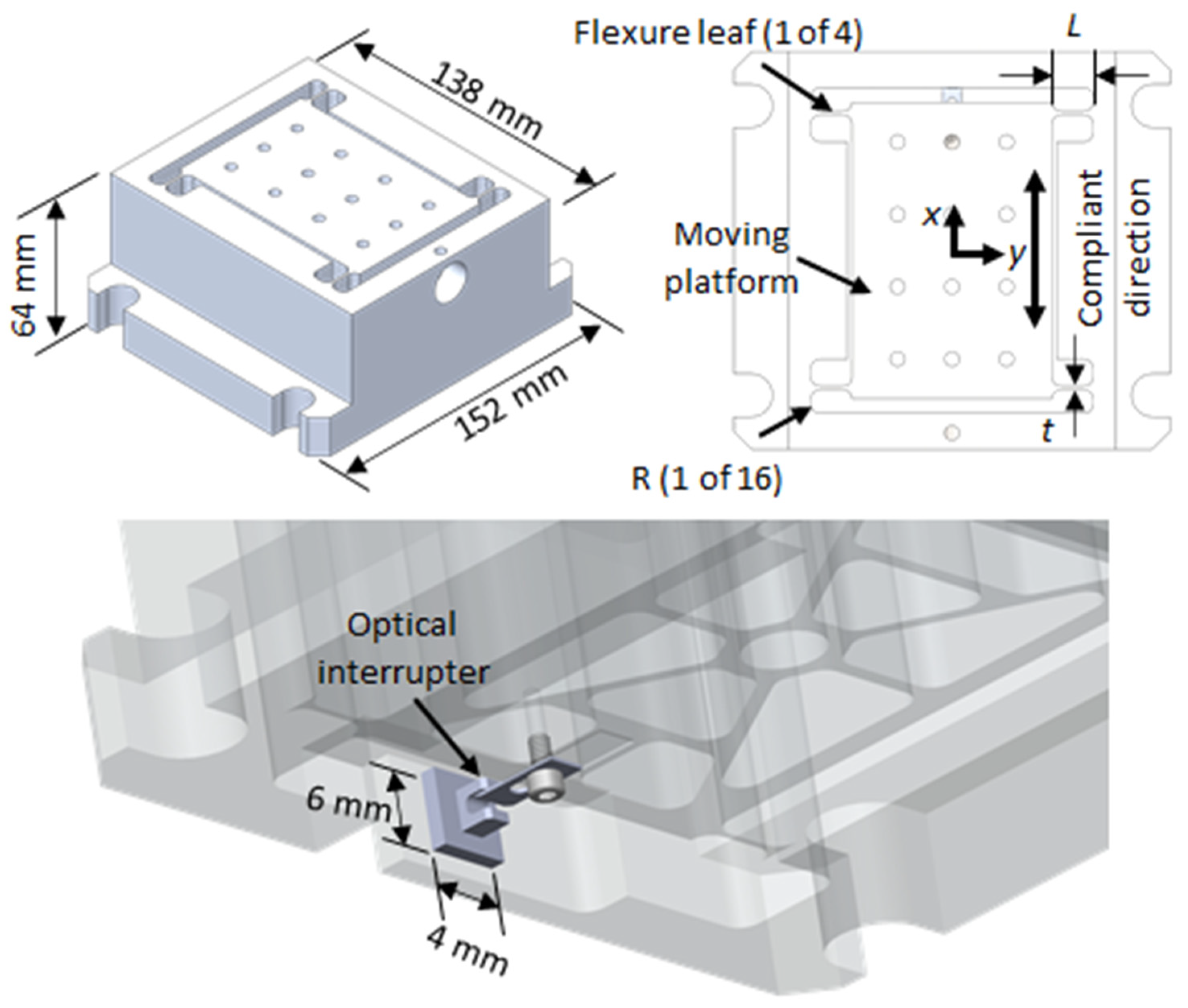
Figure 1.
Constrained-motion dynamometer design and optical interrupter placement for displacement measurement.
Figure 1.
Constrained-motion dynamometer design and optical interrupter placement for displacement measurement.
Figure 2.
Chip regeneration in milling. The feed direction is identified, and the tool rotation is assumed to be clockwise with respect to the fixed x-y coordinate system.
Figure 2.
Chip regeneration in milling. The feed direction is identified, and the tool rotation is assumed to be clockwise with respect to the fixed x-y coordinate system.
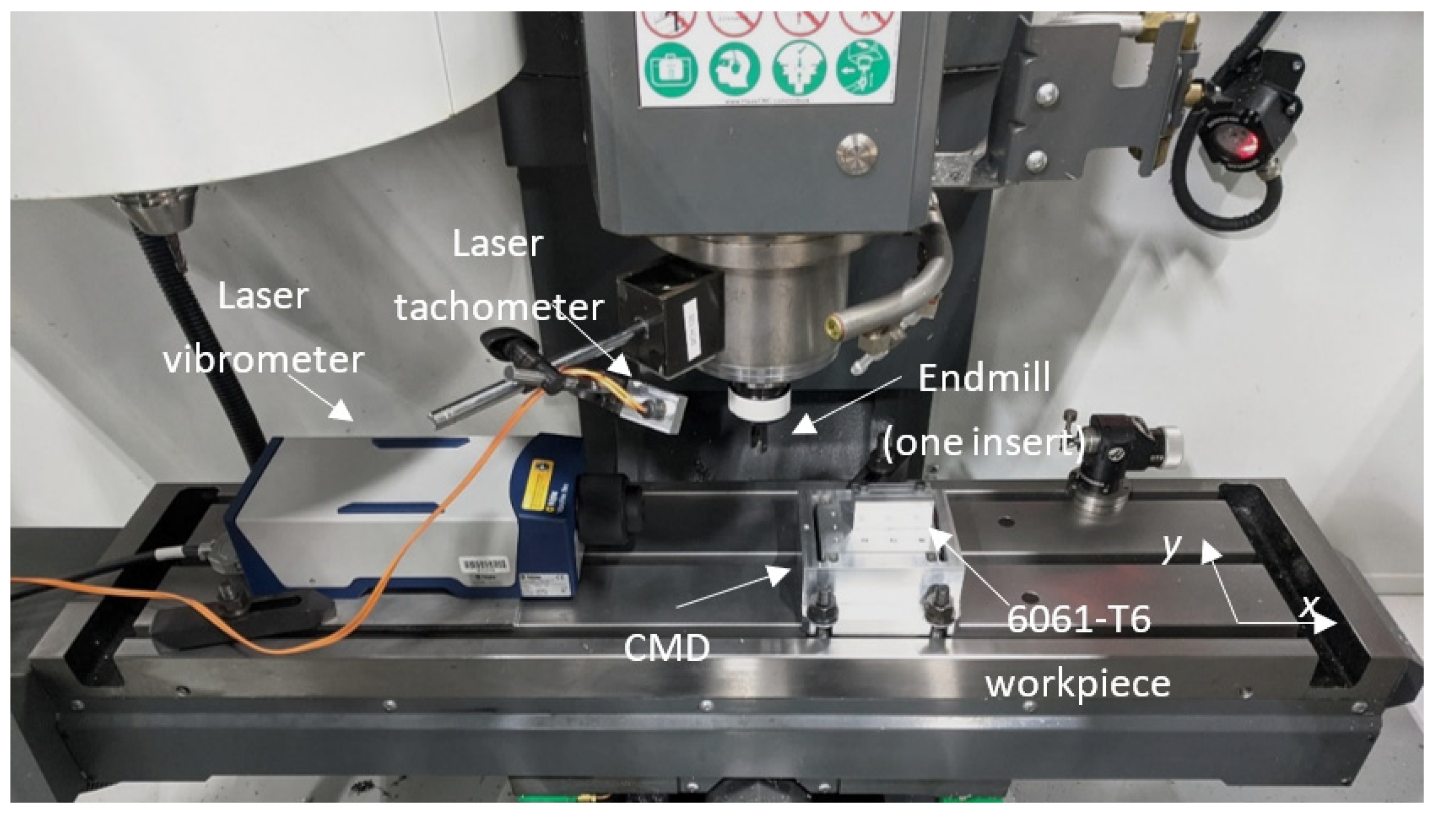
Figure 3.
Experimental setup for the milling stability validation tests.
Figure 3.
Experimental setup for the milling stability validation tests.
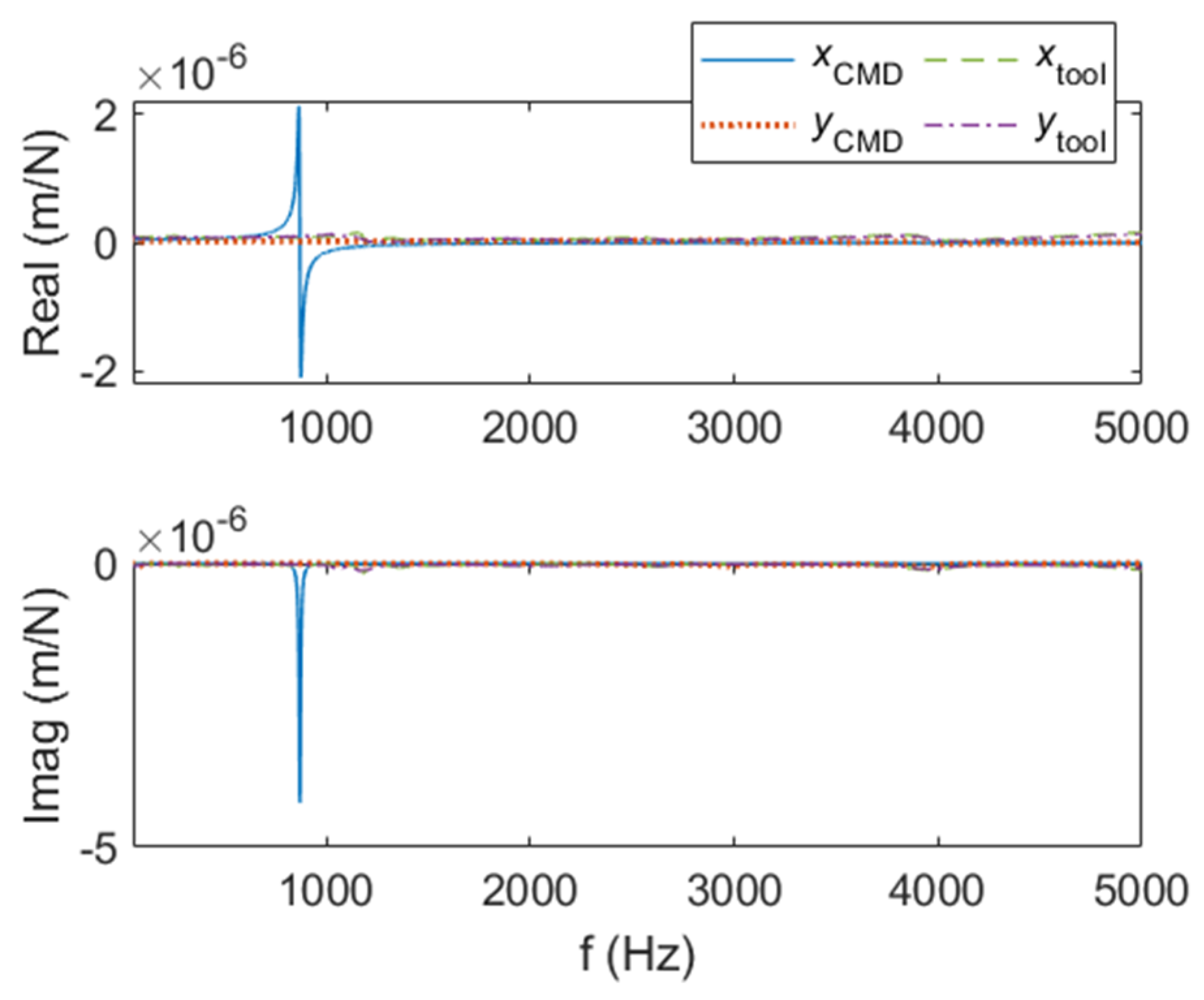
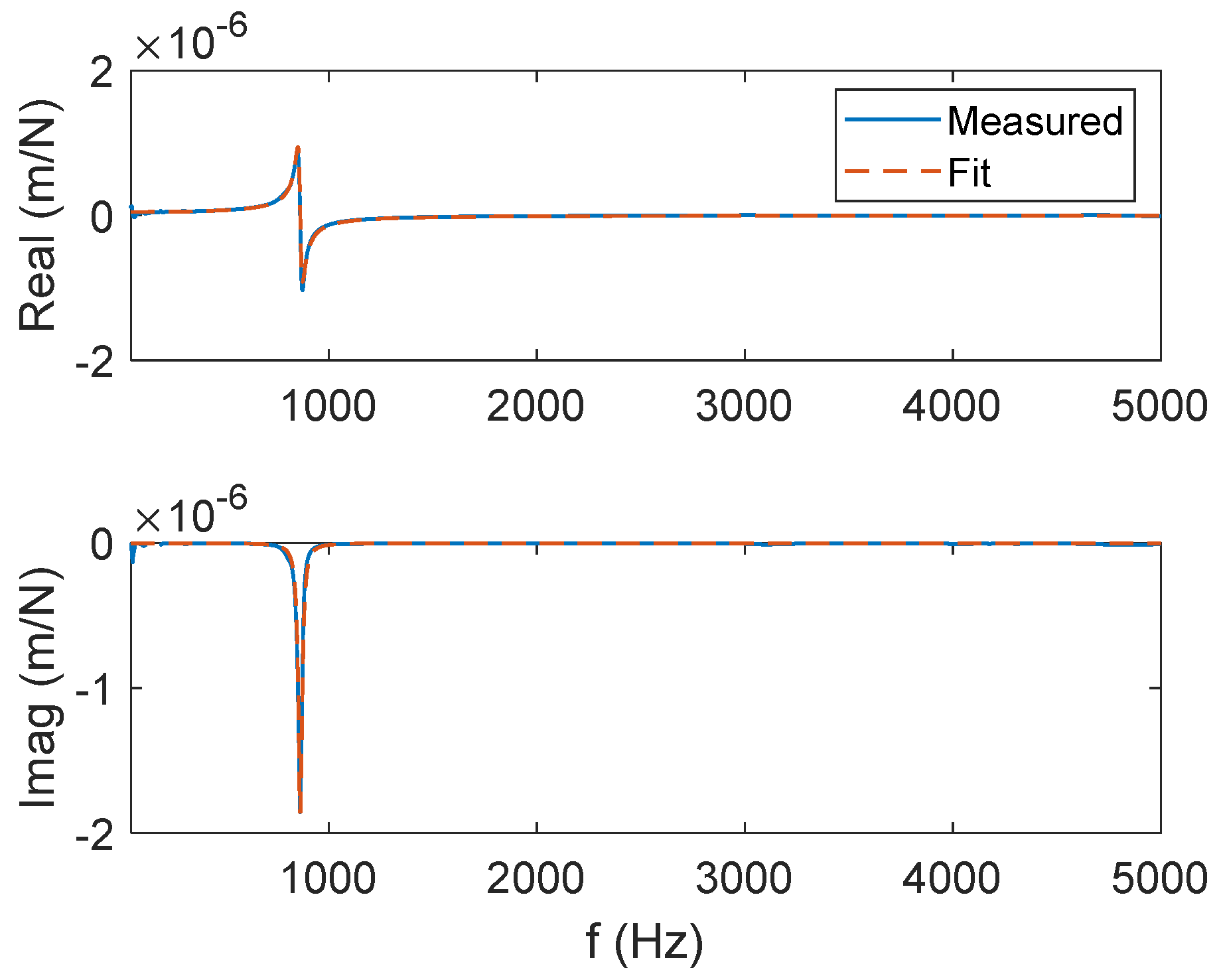
Figure 4.
Modal fit FRFs of the tool and CMD (no damping) for the stability validation setup.
Figure 4.
Modal fit FRFs of the tool and CMD (no damping) for the stability validation setup.
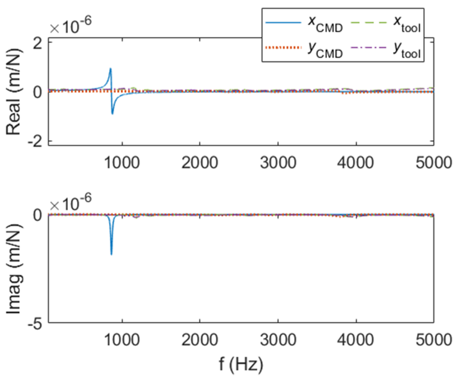
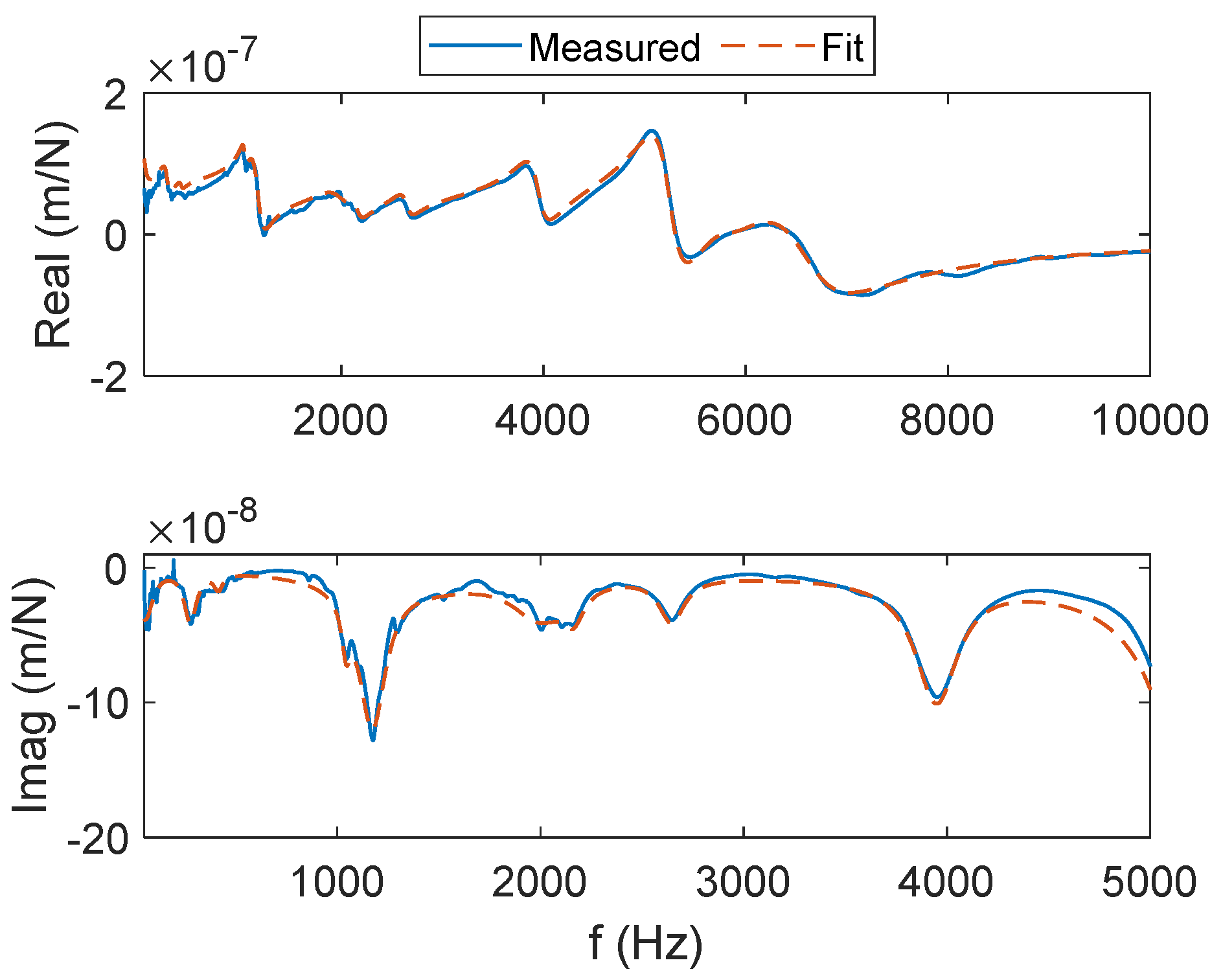
Figure 5.
Modal fit FRFs of the tool and CMD (with damping) for the stability validation setup.
Figure 5.
Modal fit FRFs of the tool and CMD (with damping) for the stability validation setup.
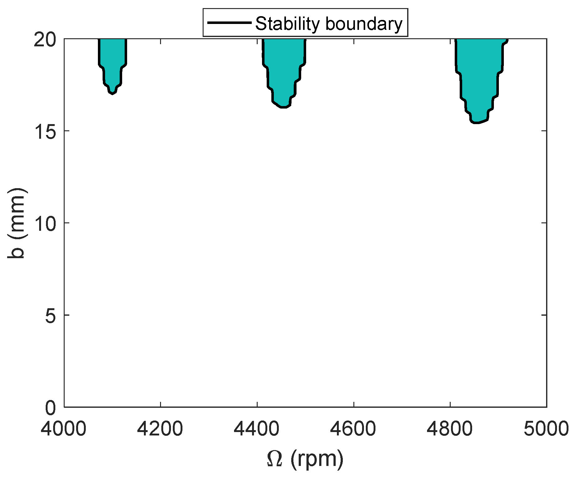
Figure 6.
Time-domain stability limit (TDS), solid black line with teal infill, expressed as a function of spindle speed, Ω, for the CMD (no damping).
Figure 6.
Time-domain stability limit (TDS), solid black line with teal infill, expressed as a function of spindle speed, Ω, for the CMD (no damping).
Figure 7.
Time-domain stability limit (TDS), solid black line with teal infill, expressed as a function of spindle speed, Ω, for the CMD (with damping).
Figure 7.
Time-domain stability limit (TDS), solid black line with teal infill, expressed as a function of spindle speed, Ω, for the CMD (with damping).
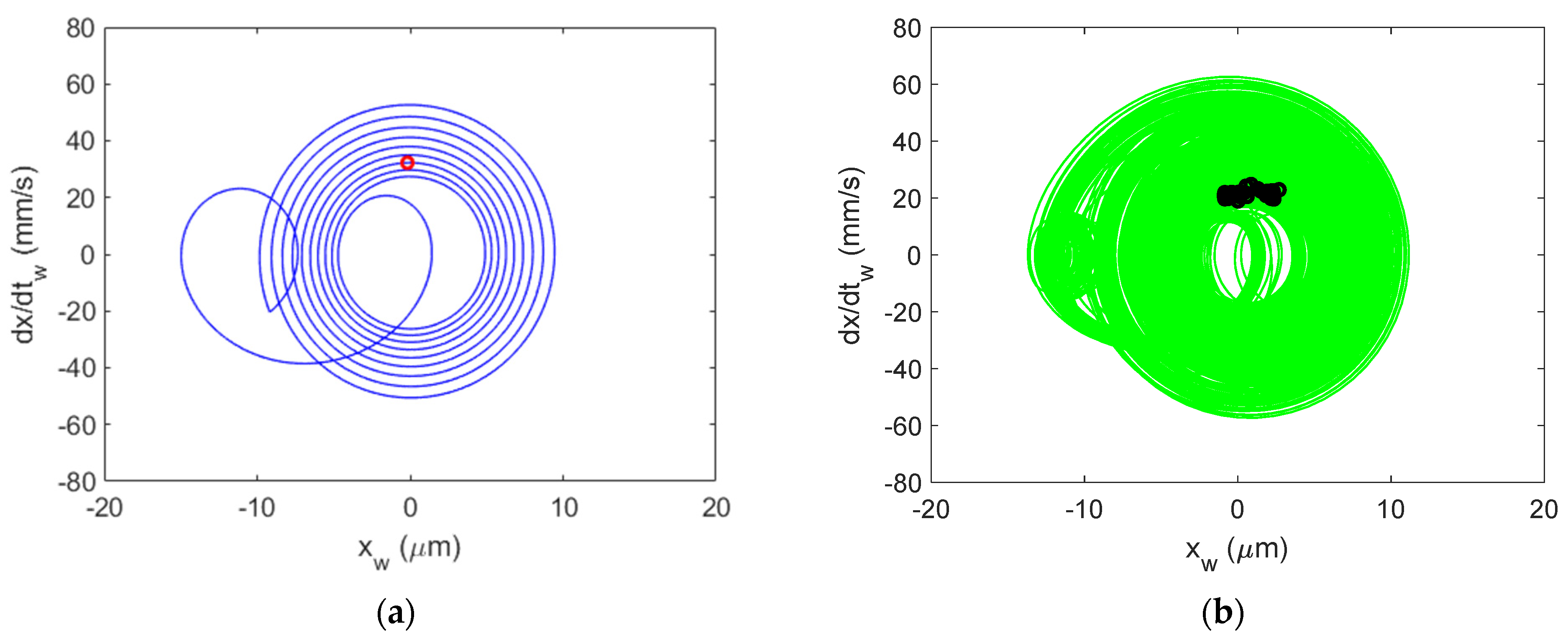
Figure 8.
Al-6061-T6 CMD (no damping) vibration behavior for stable cutting at {4900 rpm, 1 mm}. Predicted displacement (a), velocity (b), and once-per-tooth (OPT) Poincaré map (c) and measured displacement (d), velocity (e), and OPT Poincaré map (f).
Figure 8.
Al-6061-T6 CMD (no damping) vibration behavior for stable cutting at {4900 rpm, 1 mm}. Predicted displacement (a), velocity (b), and once-per-tooth (OPT) Poincaré map (c) and measured displacement (d), velocity (e), and OPT Poincaré map (f).
Figure 9.
Al 6061-T6 CMD (no damping) Poincaré maps for stable cutting at {4900 rpm, 2 mm}. Predicted (a) and measured (b).
Figure 9.
Al 6061-T6 CMD (no damping) Poincaré maps for stable cutting at {4900 rpm, 2 mm}. Predicted (a) and measured (b).
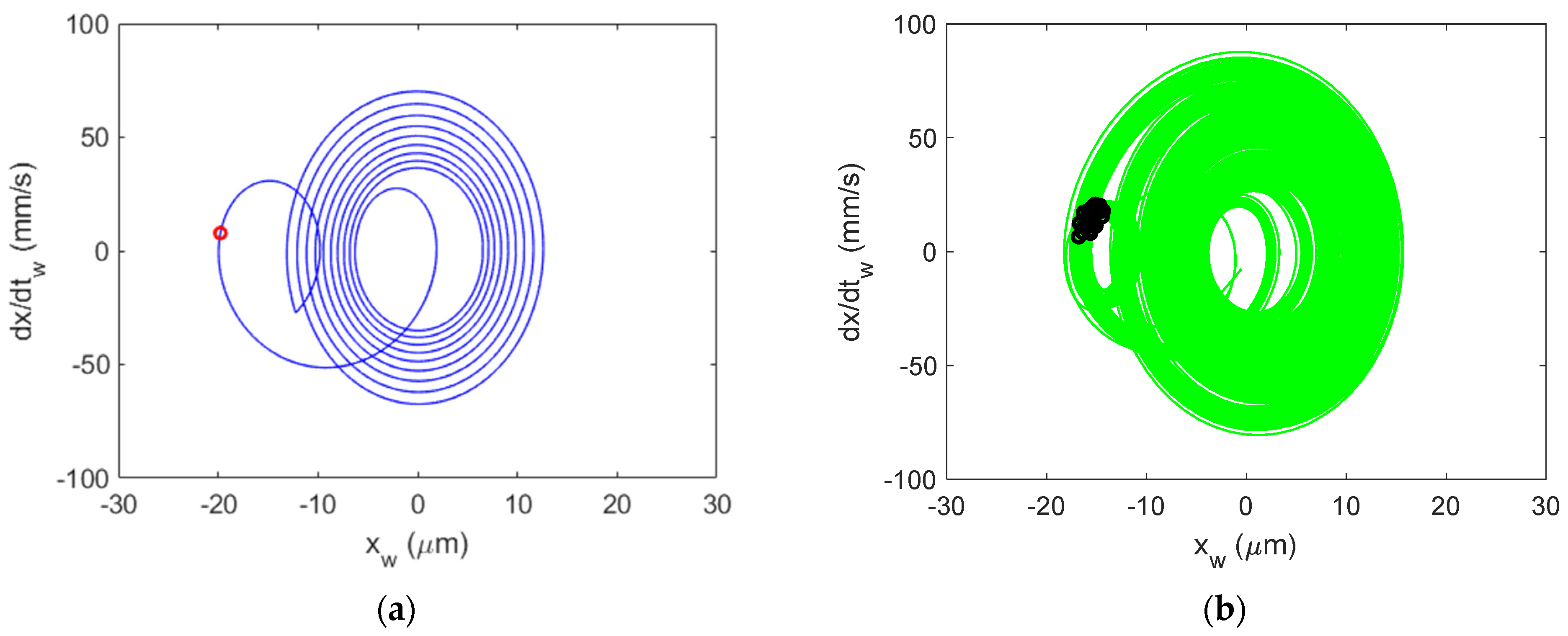
Figure 10.
Al 6061-T6 CMD (no damping) Poincaré maps for stable cutting at {4900 rpm, 3 mm}. Predicted (a) and measured (b).
Figure 10.
Al 6061-T6 CMD (no damping) Poincaré maps for stable cutting at {4900 rpm, 3 mm}. Predicted (a) and measured (b).
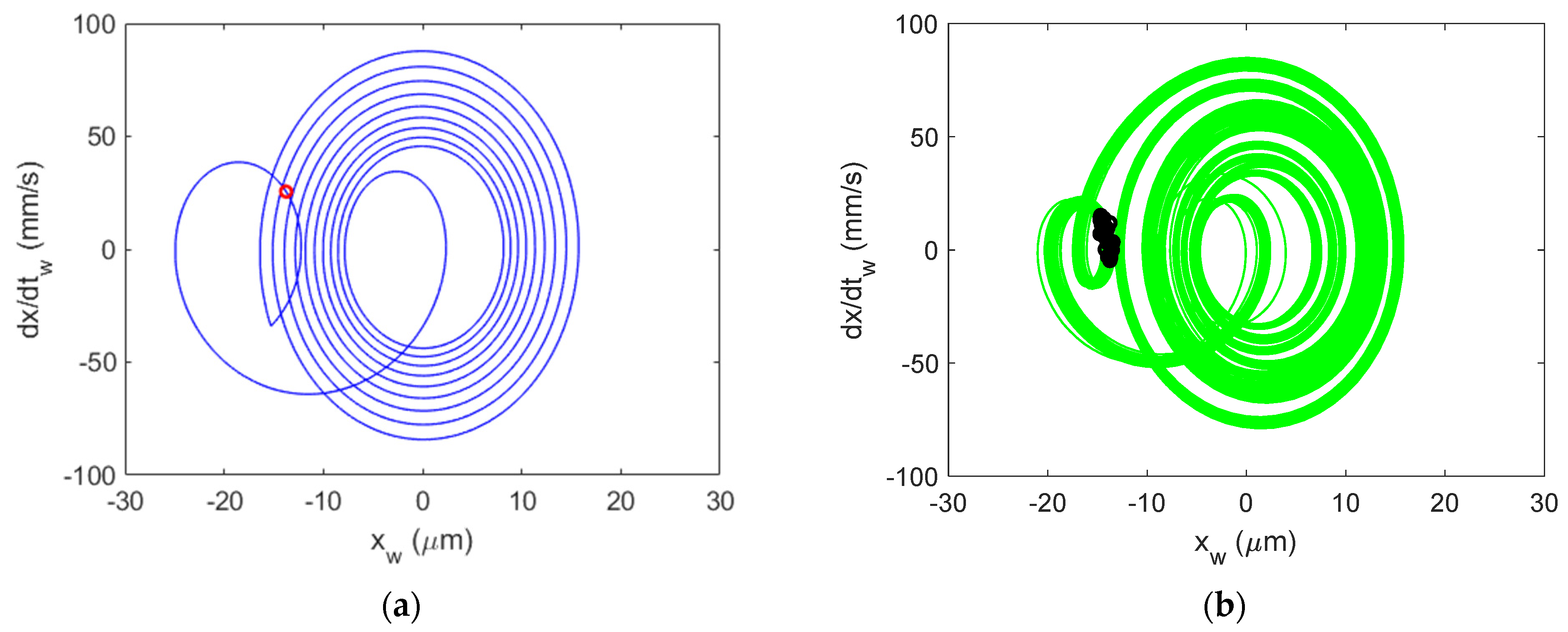
Figure 11.
Al 6061-T6 CMD (no damping) Poincaré maps for stable cutting at {4900 rpm, 4 mm}. Predicted (a) and measured (b).
Figure 11.
Al 6061-T6 CMD (no damping) Poincaré maps for stable cutting at {4900 rpm, 4 mm}. Predicted (a) and measured (b).
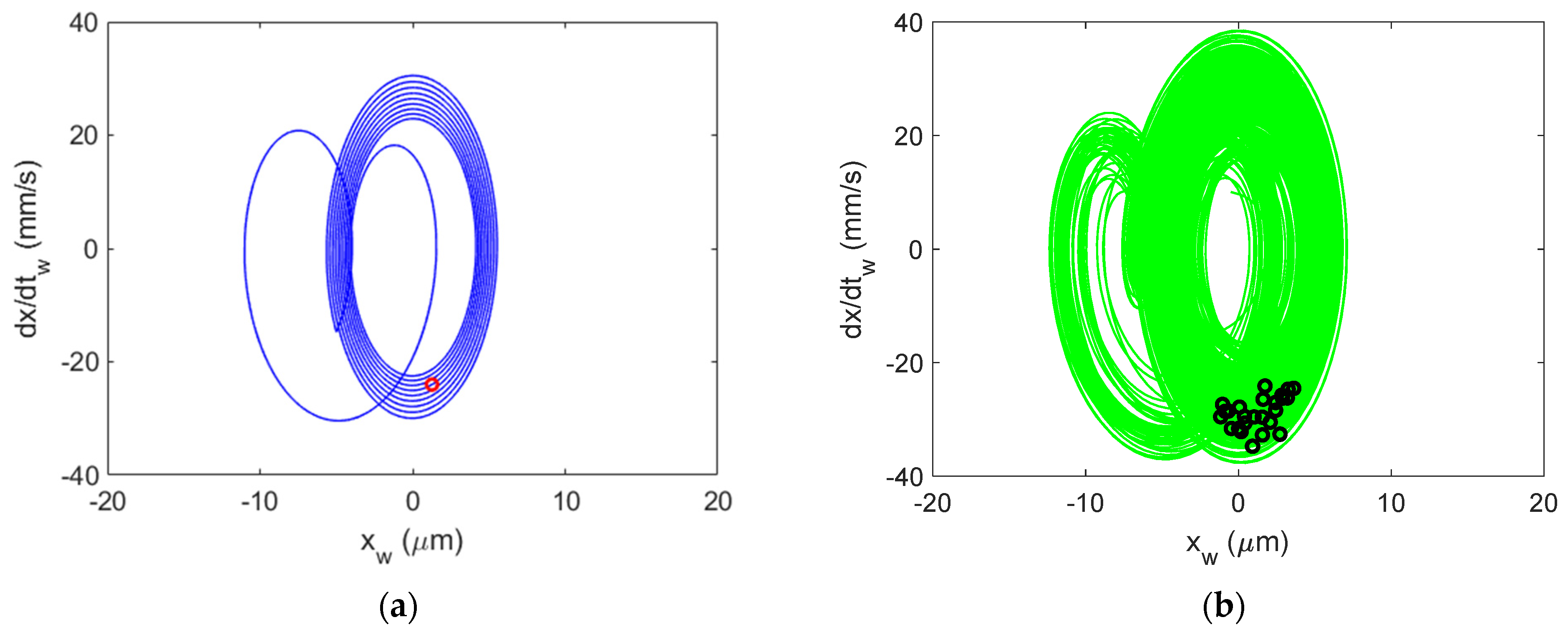
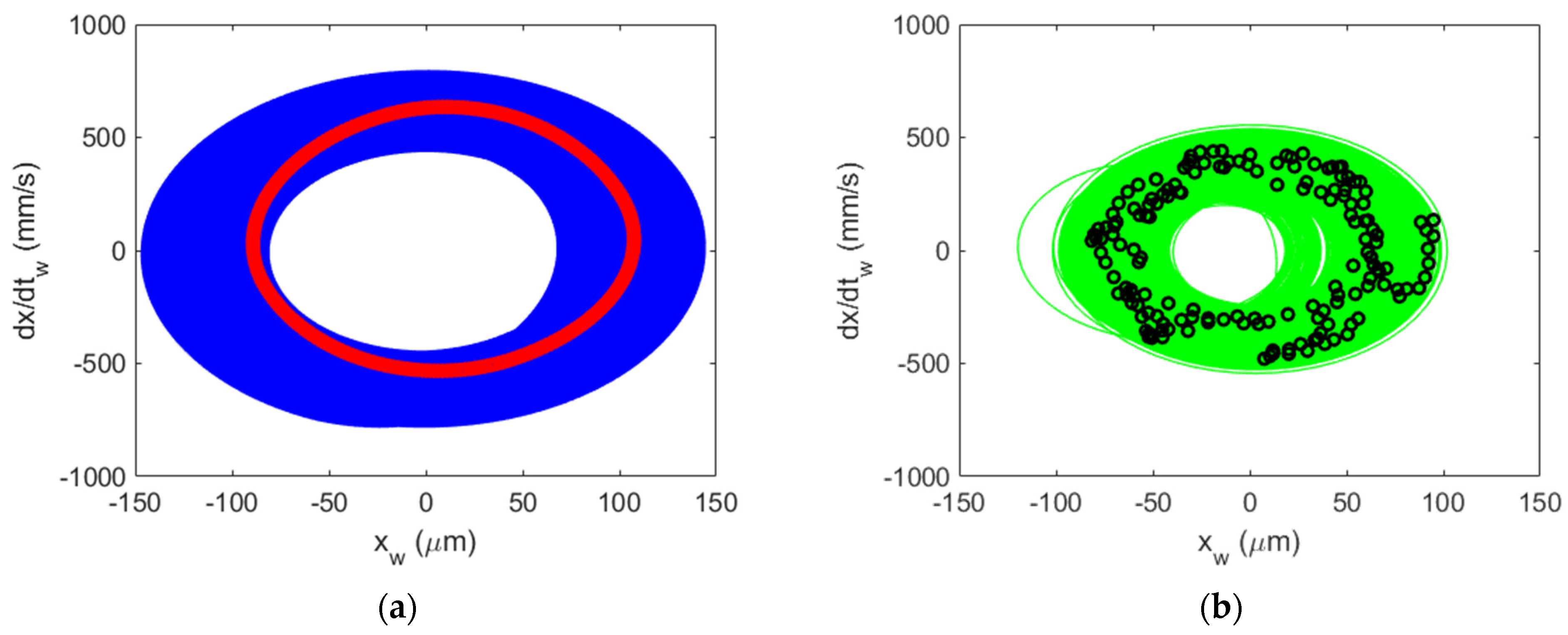
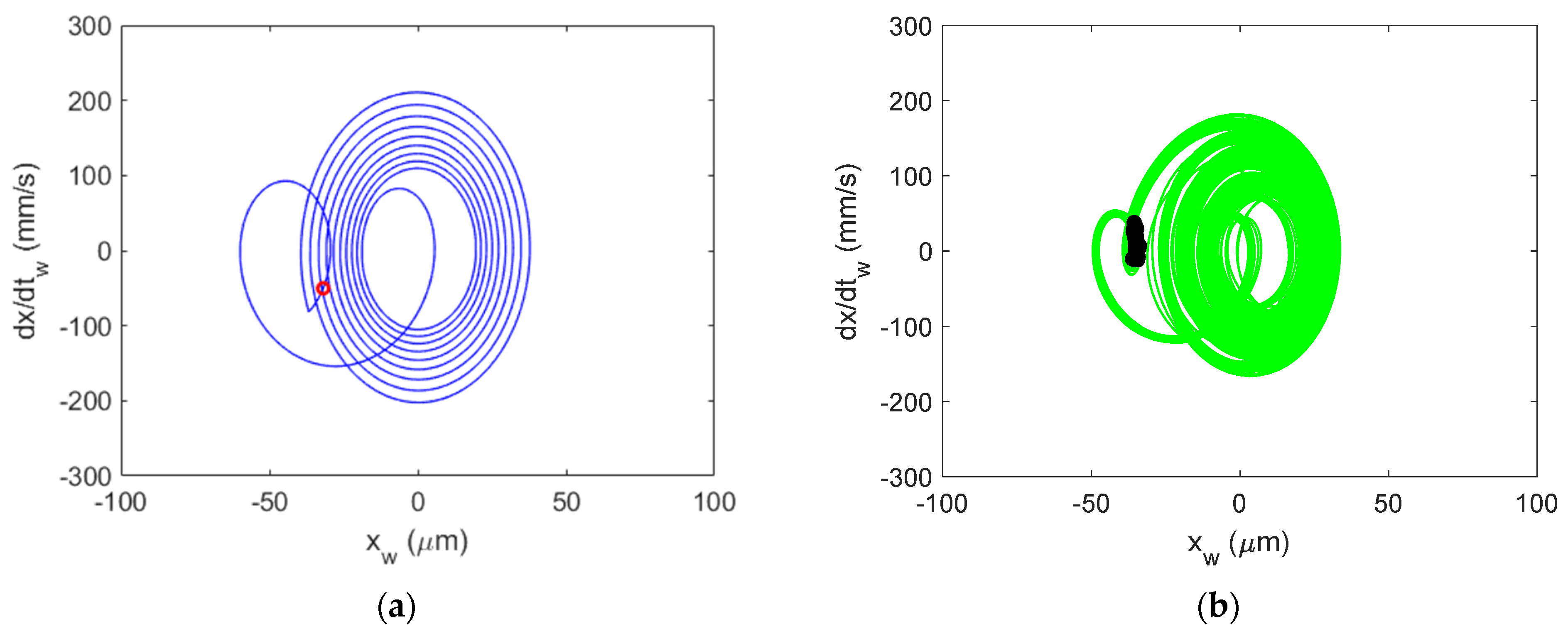
Figure 12.
Al 6061-T6 CMD (no damping) Poincaré maps for regenerative chatter (secondary Hopf bifurcation) at {4900 rpm, 5 mm}. Predicted (
a) and measured (
b). Note the difference in scale from
Figure 11.
Figure 12.
Al 6061-T6 CMD (no damping) Poincaré maps for regenerative chatter (secondary Hopf bifurcation) at {4900 rpm, 5 mm}. Predicted (
a) and measured (
b). Note the difference in scale from
Figure 11.
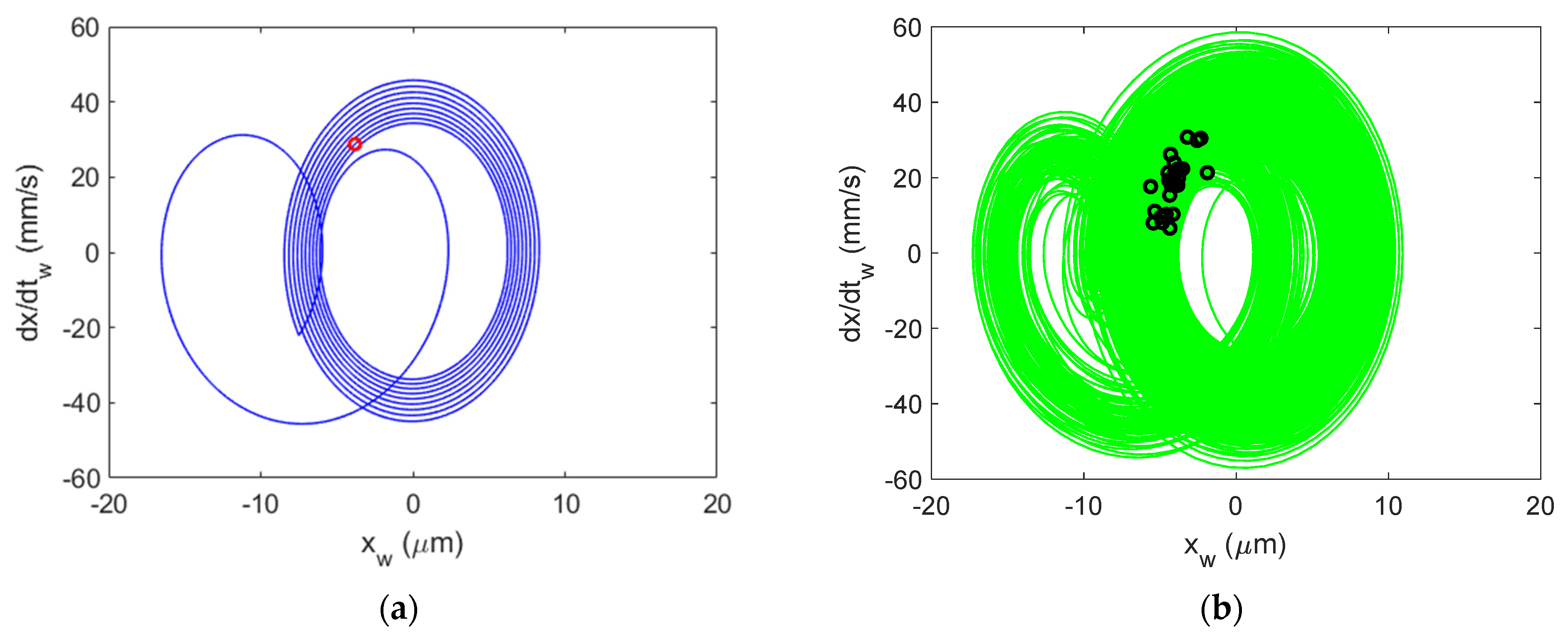
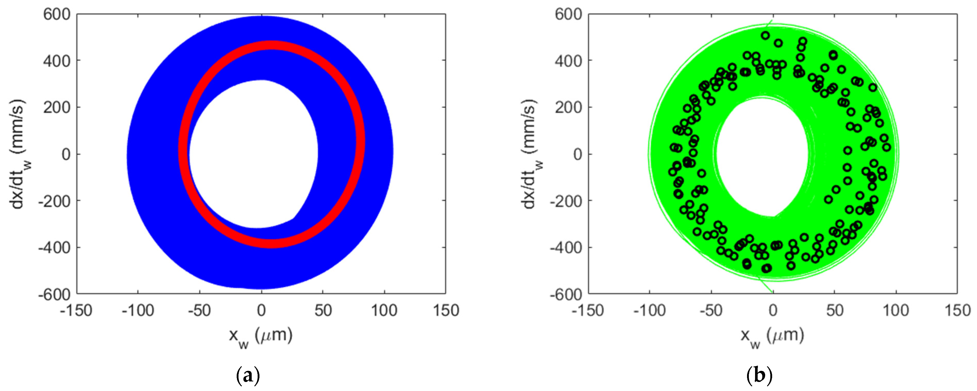
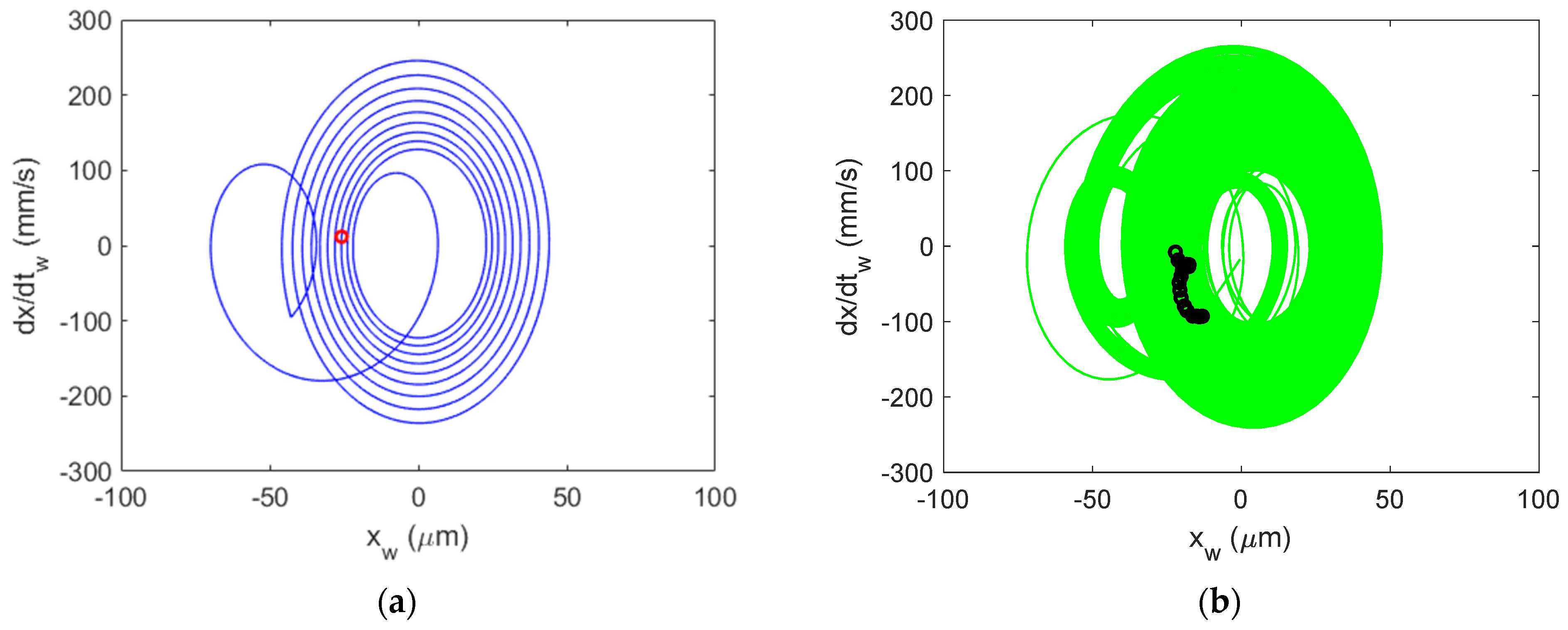
Figure 13.
Al 6061-T6 CMD (no damping) Poincaré maps for regenerative chatter (secondary Hopf bifurcation) at {4900 rpm, 6 mm}. Predicted (a) and measured (b).
Figure 13.
Al 6061-T6 CMD (no damping) Poincaré maps for regenerative chatter (secondary Hopf bifurcation) at {4900 rpm, 6 mm}. Predicted (a) and measured (b).
Figure 14.
Al-6061-T6 CMD (with damping) vibration behavior for stable cutting at {4900 rpm, 1 mm}. Predicted displacement (a), velocity (b), and OPT Poincaré map (c) and measured displacement (d), velocity (e), and OPT Poincaré map (f).
Figure 14.
Al-6061-T6 CMD (with damping) vibration behavior for stable cutting at {4900 rpm, 1 mm}. Predicted displacement (a), velocity (b), and OPT Poincaré map (c) and measured displacement (d), velocity (e), and OPT Poincaré map (f).
Figure 15.
Al 6061-T6 CMD (with damping) Poincaré maps for stable cutting at {4900 rpm, 2 mm}. Predicted (a) and measured (b).
Figure 15.
Al 6061-T6 CMD (with damping) Poincaré maps for stable cutting at {4900 rpm, 2 mm}. Predicted (a) and measured (b).
Figure 16.
Al 6061-T6 CMD (with damping) Poincaré maps for stable cutting at {4900 rpm, 3 mm}. Predicted (a) and measured (b).
Figure 16.
Al 6061-T6 CMD (with damping) Poincaré maps for stable cutting at {4900 rpm, 3 mm}. Predicted (a) and measured (b).
Figure 17.
Al 6061-T6 CMD (with damping) Poincaré maps for stable cutting at {4900 rpm, 4 mm}. Predicted (a) and measured (b).
Figure 17.
Al 6061-T6 CMD (with damping) Poincaré maps for stable cutting at {4900 rpm, 4 mm}. Predicted (a) and measured (b).
Figure 18.
Al 6061-T6 CMD (with damping) Poincaré maps for stable cutting at {4900 rpm, 5 mm}. Predicted (a) and measured (b).
Figure 18.
Al 6061-T6 CMD (with damping) Poincaré maps for stable cutting at {4900 rpm, 5 mm}. Predicted (a) and measured (b).
Figure 19.
Al 6061-T6 CMD (with damping) Poincaré maps for stable cutting at {4900 rpm, 6 mm}. Predicted (a) and measured (b).
Figure 19.
Al 6061-T6 CMD (with damping) Poincaré maps for stable cutting at {4900 rpm, 6 mm}. Predicted (a) and measured (b).
Figure 20.
Al 6061-T6 CMD (with damping) Poincaré maps for stable cutting at {4900 rpm, 7 mm}. Predicted (a) and measured (b).
Figure 20.
Al 6061-T6 CMD (with damping) Poincaré maps for stable cutting at {4900 rpm, 7 mm}. Predicted (a) and measured (b).
Figure 21.
Al 6061-T6 CMD (with damping) Poincaré maps for stable cutting at {4900 rpm, 8 mm}. Predicted (a) and measured (b).
Figure 21.
Al 6061-T6 CMD (with damping) Poincaré maps for stable cutting at {4900 rpm, 8 mm}. Predicted (a) and measured (b).
Figure 22.
Al 6061-T6 CMD (with damping) Poincaré maps for stable cutting at {4900 rpm, 9 mm}. Predicted (a) and measured (b).
Figure 22.
Al 6061-T6 CMD (with damping) Poincaré maps for stable cutting at {4900 rpm, 9 mm}. Predicted (a) and measured (b).
Figure 23.
Al 6061-T6 CMD (with damping) Poincaré maps for stable cutting at {4900 rpm, 10 mm}. Predicted (a) and measured (b).
Figure 23.
Al 6061-T6 CMD (with damping) Poincaré maps for stable cutting at {4900 rpm, 10 mm}. Predicted (a) and measured (b).
Figure 24.
Al 6061-T6 CMD (with damping) Poincaré maps for stable cutting at {4900 rpm, 11 mm}. Predicted (a) and measured (b).
Figure 24.
Al 6061-T6 CMD (with damping) Poincaré maps for stable cutting at {4900 rpm, 11 mm}. Predicted (a) and measured (b).
Figure 25.
Al 6061-T6 CMD (with damping) Poincaré maps for stable cutting at {4900 rpm, 12 mm}. Predicted (a) and measured (b).
Figure 25.
Al 6061-T6 CMD (with damping) Poincaré maps for stable cutting at {4900 rpm, 12 mm}. Predicted (a) and measured (b).
Figure 26.
Al 6061-T6 CMD (with damping) Poincaré maps for stable cutting at {4900 rpm, 13 mm}. Predicted (a) and measured (b).
Figure 26.
Al 6061-T6 CMD (with damping) Poincaré maps for stable cutting at {4900 rpm, 13 mm}. Predicted (a) and measured (b).
Figure 27.
Al 6061-T6 CMD (with damping) Poincaré maps for stable cutting at {4900 rpm, 14 mm}. Predicted (a) and measured (b).
Figure 27.
Al 6061-T6 CMD (with damping) Poincaré maps for stable cutting at {4900 rpm, 14 mm}. Predicted (a) and measured (b).
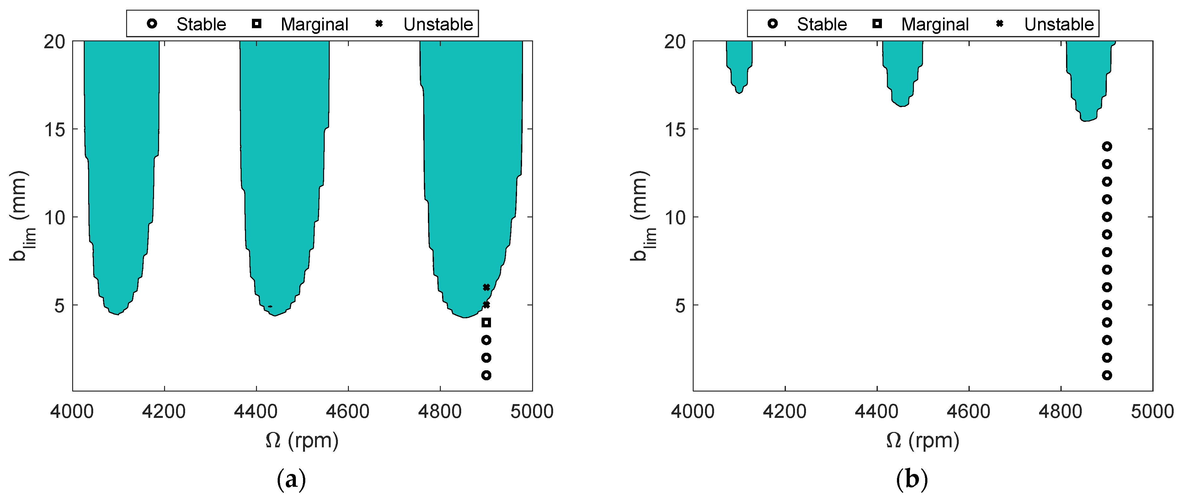
Figure 28.
Milling stability validation for the CMD (no damping) (a) and the CMD (with damping) (b).
Figure 28.
Milling stability validation for the CMD (no damping) (a) and the CMD (with damping) (b).
Figure 29.
Milling stability lobe comparison for the CMD (no damping) (a) and the CMD (with damping) (b).
Figure 29.
Milling stability lobe comparison for the CMD (no damping) (a) and the CMD (with damping) (b).
Table 1.
Comparison of different measurement principles for cutting force measurement.
Table 1.
Comparison of different measurement principles for cutting force measurement.
| Principle | Output Response | Output Quantity |
|---|
| Piezoelectric | Change piezoelectric material deformation generating charge | Electric charge, C |
| Capacitive | Change in capacitance | Electric capacitance, F |
| Inductive | Change in electromagnetic induction | Electrical potential, V |
| Piezoresistive | Change in resistance (semiconductor strain gauge) | Electrical resistance, Ω |
| Resistive | Change in resistance (wire/metal film strain gauge) | Electrical resistance, Ω |
| Drive current | Change in current consumption by the driving motors of the machine tool | Electrical current, A |
| Compliance | Change in mechanical elastic deformation | Mechanical displacement, m |
Table 2.
Tool description and cutting parameters for the milling stability validation tests.
Table 2.
Tool description and cutting parameters for the milling stability validation tests.
| Diameter (mm) | Teeth | Insert Material |
|---|
| 15.88 | 1 | Coated carbide
(Kennametal EC1402FLDJ) |
| Cutting parameters |
| Spindle speed (rpm) | 4900 |
| Feed per tooth(mm) | 0.1 |
| Axial depth (mm) | Various |
| Radial depth (mm) | 3 (19% radial immersion) |
| Cutting direction | Conventional (up) milling |
| Cutting force coefficients |
| ktc (N/mm2) | 1250 |
| krc (N/mm2) | 400 |
| kte (N/mm) | 5 |
| kre (N/mm) | 7 |
Table 3.
x-direction modal parameters for the single degree of freedom (SDOF) constrained-motion dynamometers (CMDs).
Table 3.
x-direction modal parameters for the single degree of freedom (SDOF) constrained-motion dynamometers (CMDs).
| Modal Parameters | Al 6061-T6 CMD
(No Damping) | Al 6061-T6 CMD
(with Damping) |
|---|
| Direction | x | x |
| m (kg) | 0.689 | 0.701 |
| k (N/m) | 2.08 × 10⁷ | 2.07 × 10⁷ |
| c (N-s/m) | 43 | 99 |
Table 4.
Cutting conditions and calculated stability metric, M, for the CMD (no damping).
Table 4.
Cutting conditions and calculated stability metric, M, for the CMD (no damping).
| Spindle Speed (rpm) | Radial Depth (mm) | Axial Depth (mm) | Metric, M (μm) |
|---|
| 4900 | 3 | 1 | 0.32 |
| 2 | 0.57 |
| 3 | 0.51 |
| 4 | 1.16 |
| 5 | 58.80 |
| 6 | 49.35 |
Table 5.
Cutting conditions and calculated stability metric, M, for the CMD (with damping).
Table 5.
Cutting conditions and calculated stability metric, M, for the CMD (with damping).
| Spindle Speed (rpm) | Radial Depth (mm) | Axial Depth (mm) | Metric, M (μm) |
|---|
| 4900 | 3 | 1 | 0.10 |
| 2 | 0.20 |
| 3 | 0.18 |
| 4 | 0.24 |
| 5 | 0.24 |
| 6 | 0.32 |
| 7 | 0.33 |
| 8 | 0.30 |
| 9 | 0.88 |
| 10 | 0.31 |
| 11 | 0.73 |
| 12 | 0.36 |
| 13 | 0.34 |
| 14 | 0.83 |


