Influence of Constitutive Models and the Choice of the Parameters on FE Simulation of Ti6Al4V Orthogonal Cutting Process for Different Uncut Chip Thicknesses ^†

Abstract

The constitutive model and its pertinent set of parameters are important input data in finite element modeling to define the behavior of Ti6Al4V during machining process. The present work focusses on comparing different constitutive models and the parameters sets available in literatures and investigating the quality of the predictions when varying uncut chip thickness (40 µm, 60 µm, 100 µm and 280 µm). In addition, temperature-dependent strain hardening factor along with strain softening phenomenon based reconstructed material model is proposed. The results from the numerical simulations are compared with experimental results available in literature. The comparison shows that the force values are highly influenced by constitutive models and the choice of parameters sets, whereas the chip morphologies are mainly influenced by the uncut chip thickness and constitutive models. This work justifies the need for an appropriate set of parameters and constitutive model that replicate the machining behavior of Ti6Al4V alloy for different cutting conditions.

1. Introduction

The titanium alloy, especially Ti6Al4V, is one of the most important and commonly used alloys for its attractive properties in aerospace, biomedical, submarine applications, etc. as it exhibits elevated strength, low density, good corrosion resistance, excellent high temperature properties [1,2]. Most of mechanical components with titanium alloys, are produced with machining operation [1,3]. The conventional machining process of Ti6Al4V has proved to be particularly complex due to its inherent properties such as, low thermal conductivity and high reactivity along with the diversity of physical phenomena involved, including large elasto-plastic deformation, complex contact/friction conditions, thermo-mechanical coupling and chip separation mechanisms [4,5,6]. Highspeed machining of Ti6Al4V alloy is still the interest of many researchers even after many decades of research [4]. The direct measurements of the stress, the strain, the strain rate and the temperature in the small deformation zone during chip formation are extremely difficult to assess experimentally [5]. So numerical techniques are often used. Finite element modeling is the most significant and extensively used numerical technique that is employed to investigate thermomechanical phenomena and nonlinearities involved in the simulation of machining process [6,7,8].

Since the early 1980s the numerical models are usually based on Lagrangian and Eulerian formulations [9,10]. In Eulerian formulation, the mesh is fixed in space and the material flows through the element that avoids critical element distortion. The main limitation of Eulerian model is that the chip geometry must be known in advance. The Lagrangian formulation has been extensively used by the researchers to simulate the chip geometry from the incipient stage to a steady state despite its drawback on mesh distortion problems [4,9,10]. These Lagrangian models require a separation criterion to remove the chip from the work piece. The separation criterions are based on either the geometrical considerations or the physical considerations. The geometrical method criterion is based on the chip separation along a predefined cutting plane and the physical method criterion is based on the chip separation using element deletion [11,12]. The Lagrangian models are also used with mesh adaptivity and automatic remeshing to eliminate the need for the chip separation criterion [13]. Consequently, this leads to an increase in the computation time [9,10].

More recent advanced numerical formulations such as the Arbitrary Lagrangian-Eulerian (ALE) formulation and Coupled Eulerian–Lagrangian (CEL) that take the best features of Lagrangian and Eulerian formulations have been implemented by Ducobu et al. [14,15] for modelling the orthogonal cutting process of Ti6Al4V alloy. In [15], the authors implemented Lagrangian, ALE and CEL formulations for different uncut chip thicknesses that produce continuous chips and showed that the results from ALE and CEL models are in good agreement with the experimental results with the reduction in computation time. The progression in the computational environments led the researchers to move from simple 2D to complex 3D finite element model of cutting process. Ducobu et al. [16] extensively discussed on 3D FE models that are implemented in the study of cutting process and developed a 3D finite element Coupled Eulerian–Lagrangian model that replicates the experimental cutting operation of Ti6Al4V alloy. For this study, an explicit Lagrangian finite element model with 2D assumption [7,17] is considered for the simulation of cutting process.

The mechanics of cutting process examines the deformation of a workpiece subjected to machining, such as chip formation, machining forces, residual stresses, temperature effects, strain rate effects and surface integrity [4]. A reliable constitutive material model is essential to relate to the large plastic strains at the very high strain rates and the very high temperatures observed during machining process [4,18,19]. So far, several empirical and physical based models have been developed and are employed by the researchers when machining of Ti6Al4V alloy, in which empirical models are mostly recommended for their flexibility, robustness and large availability of data’s [4,20]. The Johnson–Cook (JC) [21] material model coupled with JC damage criterion [22] are highly employed for machining simulation. Mostly, the parameters identified for this law is by the experiments for testing the dynamic stress–strain response of materials that are fitted to stress strain curve [23]. These experiments can reach maximum strain of 0.5 and strain rate near to 10³ s⁻¹ which is well below the strain of 3 or even higher and the strain rate above 10⁵ that are actually evident during cutting process. The resulting extrapolation leads to loss of some important information [24]. To solve this issue, many modified JC empirical models are proposed [25,26,27].

The parameters values that are implemented in constitutive models is the another most significant input that directly influence the simulated results. The availability of different sets of parameters in literatures raises the concern [28,29] which initiates the discussion on the influence of parameters sets and their impacts on the results. In [29], the authors justify the influence of the parameters set for a single cutting condition with three different constitutive model. In this present article the work is further extended with three other cutting condition along with the influence of four different constitutive models.

This paper investigates the finite element simulated results from

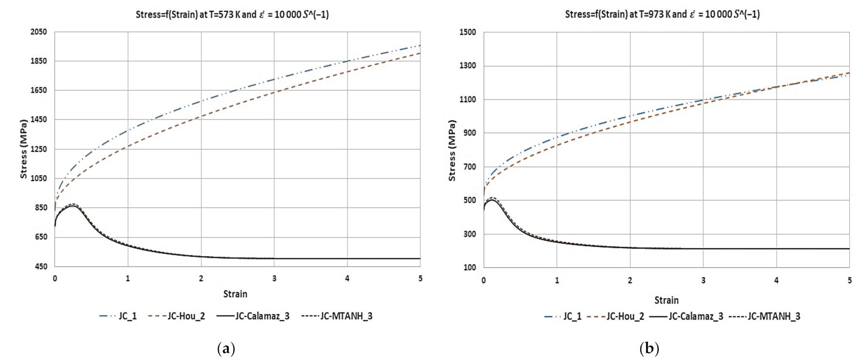
• The Johnson–Cook model [21].
• The Modified Johnson–Cook model from Calamaz et al. [25] that considers the strains softening phenomenon.
• The Modified Johnson–Cook model from Hou et al. [30] that takes into account temperature dependent hardening aspect and its coupled effects between strain and temperature.
• A reconstructed material model proposed in this study to figure out the influence of temperature hardening effect on the model proposed by Calamaz et al. [25]. The model combines strain softening phenomenon from Calamaz et al. [25] and temperature dependent hardening effect from Hou et al. [30].

These constitutive models are employed with three different sets of parameters acquired from Seo et al. [31], Calamaz et al. [25] and Hou et al. [30] Each constitutive model is analyzed with three different sets of parameters making a total of twelve models. These twelve models are investigated with four different uncut chip thicknesses (40 µm, 60 µm, 100 µm and 280 µm) while the rest of the cutting conditions are unaltered throughout the study. This work aims to highlight the effect on the results of the choice of the constitutive models and the parameters sets for uncut chip thicknesses ranging from small uncut chip thicknesses (h = 40 µm, 60 µm and 100 µm) that produce continuous chips to large uncut chip thickness (h = 280 µm) that produces serrated chip for the cutting speed of 30 m/min. This is necessary as it is currently still a challenge to predict the change in the chip morphology and to model the cutting forces without changing the parameters of the finite element model. The cutting force, feed force, chip morphologies and chip thickness measured from numerical simulations are compared and are validated with the experimental results that are acquired from Ducobu et al. [32].

2. Material Models

The empirical or phenomenological constitutive model is considered by many researchers for its mathematical simplicity and flexibility, which reflects the behavior of the material observed experimentally. These models consider the variables of deformations such as the plastic strain ε, plastic strain rate $\dot{\epsilon }$ and temperature T under macroscopic scale. The general form is:

$$\sigma =\sigma \left(\epsilon ,\dot{\epsilon },T\right),$$

(1)

2.1. Johnson–Cook Constitutive Model (JC)

The Johnson–Cook model [21] is a well-known empirical formulation which is heavily exploited in modeling and simulation of orthogonal machining. The JC model is widely employed by many researchers to determine the behavior of the material during machining process for its simple form and robustness. The Johnson–Cook flow stress equation links the plastic term, viscous term and softening term. Its flow stress equation is represented by the following equation:

$$\sigma =\left[A+B{\epsilon }^n \right] \left[1+Cln\frac{\dot{\epsilon }}{{\dot{\epsilon }}_0}\right]\left[1-{\left(\frac{T-T_{room}}{T_{melt}-T_{room}}\right)}^m\right],$$

(2)

where $A$ is the yield stress at reference temperature, $B$ is the modules of strain hardening, $n$ is the strain-hardening exponent, $C$ the strain rate sensitivity and m is the thermal softening exponent. $T$ is the current temperature, $T_{melt}$ and $T_{room}$ are the melting temperature and the room temperature, respectively, while ${\dot{\epsilon }}_0$ is the reference strain rate.

$A,B,C,n,m$ are the constants that depend on the material and are determined by flow stress data obtained from material tests.

Even though the JC model is globally accepted, there are some noticeable drawbacks when considered for machining process simulations. The JC model describes the strain hardening phenomenon as an increasing function and it does not account for the softening behavior observed at the strains and temperatures in the primary shear zone regardless of the material. This leads to modified or updated versions of Johnson–Cook model to capture the unique behavior exhibited by certain alloys such as Ti6Al4V.

2.2. Modified Johnson–Cook Model by CALAMAZ (JC-Calamaz)

A modified version has been suggested by Calamaz et al. [25] taking into account the strain-softening phenomenon related to the recrystallization and dynamic recovery mechanism. The model includes novel multiplicative strain and temperature dependency by adding a hyperbolic tangent (TANH) term into the Johnson–Cook flow stress model. The material flow stress for TANH model is expressed by the following equation:

$$\sigma =\left[A+B {\epsilon }^n\left(\frac{1}{exp\left({\epsilon }^a\right)}\right)\right] \left[1+Cln\frac{\dot{\epsilon }}{{\dot{\epsilon }}_0}\right]\left[1-{\left(\frac{T-T_{room}}{T_{melt}-T_{room}}\right)}^m\right]\left[D+\left(1-D\right)tanh\left(\frac{1}{{\left(\epsilon +S\right)}^c}\right) \right]$$

(3)

where, $D=\left[1-{(T/T_{melt})}^d\right]$ and $S=[1-\left(T/T_{melt}{)}^b\right] ,$ parameters $A,B,C,n,m$ have the same meaning as for JC model and the new constants $a, b, c$ and $d$ are introduced by TANH law. The authors concluded that the TANH law significantly improves the prediction of chip morphology and suggested for the optimization of parameters for accurate prediction of the cutting force feed forces and the shear band frequencies.

2.3. Modified Johnson–Cook Model by HOU (JC-Hou)

A modified JC model is proposed by Hou et al. [30] by considering a temperature dependent strain hardening factor. JC model is altered by coupling temperature with the strain hardening factor in the strain function of JC model. This implies that when the temperature increases, the strain hardening rate decreases. The authors mentioned that the strain hardening rate $Q$ of Ti6Al4V alloy has no noticeable strain rate sensitivity but has apparent temperature sensitivity. Strain or work hardening rate $Q$ is a function of temperature:

$$Q= B\left(1+m_{1 }ln\frac{T}{T_{room}}\right)$$

(4)

The flow stress equation is expressed by the following equation:

$$\sigma =\left[A+B \left(1+m_{1 }\ln \frac{T}{T_{room}}\right){\epsilon }^n\right] \left[1+Cln\frac{\dot{\epsilon }}{{\dot{\epsilon }}_0}\right]\left[1-{\left(\frac{T-T_{room}}{T_{melt}-T_{room}}\right)}^m\right]$$

(5)

where B is the hardening modulus, $m_1$ is the thermal sensitivity coefficient with the increasing strain and the rest of the parameters have the same meaning as for JC model. The author concluded that the strain-hardening rate is dependent on the temperature.

2.4. Modified TANH Material Model (JC-MTANH)

A reconstructed JC-Calamaz model is introduced in this paper. It combines the effect of temperature dependent hardening phenomenon proposed by Hou et al. [30] along with hyperbolic function introduced by Calamaz et al. [25] observed during high-speed machining process. The equation is constructed by introducing a temperature function into the work hardening term (proposed by Hou et al. [30]) along with flow softening at higher strain (proposed by Calamaz et al. [25]). The flow stress equation is expressed by the following equation:

$$\sigma =\left[A+B{\epsilon }^n\left(1+m_{1 }\ln \frac{T}{T_{room}}\right) \left(\frac{1}{exp\left({\epsilon }^a\right)}\right)\right] \left[1+Cln\frac{\dot{\epsilon }}{{\dot{\epsilon }}_0}\right]\left[1-{\left(\frac{T-T_{room}}{T_{melt}-T_{room}}\right)}^m\right]\left[D+\left(1-D\right)\tanh \left(\frac{1}{{\left(\epsilon +S\right)}^c}\right) \right],$$

(6)

where, ${\mathrm{m}}_1$ is the thermal sensitivity coefficient with the same meaning as for JC-Hou and $D=\left[1-{(T/T_{melt})}^d\right]$, $S=[1-\left(T/T_{melt}{)}^b\right]$ come from JC-Calamaz model. The rest of all other parameters meaning is the same as for JC model.

3. Constitutive Models Parameters for Modeling of Machining Process of Ti6Al4V

The behavior of the material during machining process is determined by the constitutive model and its parameters. The values of the parameters are significantly important in predicting the results. The parameters for the models are usually identified by curve fitting of experimental stress–strain plot, this leads to some discrepancies in the parameters identification. In fact, there are plenty of parameters sets available in the literatures for the same material. This leads to the discussion on identification of right parameters set to simulate the results.

In this context, Ducobu et al. [28] extensively analyzed 20 different sets of Johnson–Cook parameters available in the literature for Ti6Al4V by comparing the outputs of a Coupled Eulerian–Lagrangian orthogonal cutting model with the experimental results. They concluded that the parameters set from Seo et al. [31] is well capable of producing near accurate results for the forces and chip thickness. From the above discussion, the set of parameters for JC model is adopted from Seo et al. [31], set of parameters for JC-Hou comes from Hou et al. [30] and the set of parameters for JC-Calamaz is adopted from the work of Calamaz et al. [25]. The sets of parameters are mentioned as 1, 2 and 3, respectively, throughout the article and their values are reported in

Table 1. Sets of parameters considered for this study—set 1 [31], set 2 [30] and set 3 [25].

1		2		3
$A$ (MPa)	997.9	$A$ (MPa)	920	$A$ (MPa)	968
$B$ (MPa)	653.1	$B$ (MPa)	400	$B$ (MPa)	380
$C$	0.0198	$C$	0.042	$C$	0.02
$m$	0.7	$m$	0.633	$m$	0.577
$n$	0.45	$n$	0.578	$n$	0.421
$T_{room}$ (K)	298	$T_{room}$ (K)	293	$T_{room}$ (K)	298
$T_{melt}$ (K)	1878	$T_{melt}$ (K)	1933	$T_{melt}$ (K)	1878
		$m_1$	0.158	$a$	1.6
				$b$	0.4
				$c$	6
				$d$	1

.

The values of $m_1$, $a$, $b$, $c$, $d$ identified by Hou et al. [30] and Calamaz et al. [25] are kept constant for all models if the constitutive equation uses these parameters. Only the common parameters are such as $A,B,C,n,m$ $T_{melt}$ and $T_{room}$ are interchanged and are represented correspondingly as 1, 2 and 3. In order to highlight the influence of parameters sets on numerical modeling of cutting process simulation the three different sets of parameters are considered with the four constitutive models.

The evolution of stress–strain curve is plotted at fixed temperatures of $T$ = 573 K and $T$ = 973 K for strain rate of $\dot{\epsilon }$= 10,000 s⁻¹ in Figure 1a and Figure 1b, respectively. JC model with set 1 parameters (JC_1), JC-Hou with set 2 parameters (JC-Hou_2), JC-Calamaz with set 3 parameters (JC-Calamaz_3) and JC-MTANH with set 3 parameters (JC-MTANH_3) along with $m_1$ identified by Hou et al. are considered.

From the evolution of stress–strain curves in Figure 1 and Figure 2. It is evident that at high strain and high temperature the JC-Calamaz law takes the softening behavior into account and the JC-Hou law that considers the temperature dependent hardening effect shows a significant difference in the evolution of flow stress at higher temperature and strain rate. The difference in the stress levels might influence the result. Indeed, it is essential to note that the initial stress value of JC-Calamaz_3 and JC-MTANH_3 is very low when compared with initial stress value of the other two constitutive models considered in this study and this could significantly influence the numerical results. From the stress strain curves, it is seen that the influence of introducing temperature dependent strain hardening term in JC-Calamaz law is less significant, but this is further discussed with numerical simulations.

The stress–strain evolutions are observed at two different temperatures. When temperature increases from 573 K to 973 K the stress level decreases as expected, confirming the presence of thermal softening phenomenon.

Figure 2 shows the flow stress evolution curves for the four constitutive models with three different sets of parameters, respectively. When compared, the stress–strain evolution with set 3 parameters shows a low initial stress value regardless of the constitutive laws, while the other sets of parameters show approximately the same initial stress value. However, JC-Hou_1 shows higher stress value with respect to increasing strain. This confirms the influence of temperature dependency in strain hardening.

The stress strain evolution curves confirm the influence of the choice of the sets of parameters for each constitutive model and their capability in influencing the results.

4. Experimental Reference

The Experimental reference is considered from the work performed by Ducobu et al. [32] on orthogonal cutting of Ti6Al4V on a high-speed milling machine shown in Figure 3.

Each cutting test was performed for 0.02 s, the time required to travel the 10 mm length. Four values of the depth of cut are considered with cutting speed of 30 m/min. The cutting conditions of the experimental tests are given in

Table 2. Cutting conditions of the experiments [32].

Cutting speed (m/min)	30
Uncut chip thickness (µm)	40, 60, 100, 280
Width of cut (mm)	1
Length of cut (mm)	10
Rack angle (°)	15
Clearance angle (°)	2
Cutting edge radius (µm)	20

.

The chips were observed with an optical microscope. Globally, continuous chips were observed for the uncut chip thicknesses of 40 µm, 60 µm and 100 µm even if very small and irregular teeth along its entire length are noticed. For uncut chip thickness of 280 µm saw toothed or serrated chips are observed with similar teeth. The chip morphology for 280 µm with a magnification factor 50 and for 40 µm, 60 µm and 100 µm with a magnification factor of 200 is shown in Figure 4.

The cutting forces are measured in the three directions with a Kistler 9257B dynamometer. The RMS cutting force (Fc), feed force (Ff) and cut chip thickness ($h^{\prime }$) measured from the experimental results are given in

Table 3. Forces and chip thickness measured from experiments for $h$ = 40 µm, 60 µm and 100 µm [32].

$\mathit{h}$ (µm)	RMS Fc (N/mm)	RMS Ff (N/mm)	${\mathit{h}}^{\prime }$ (µm)
40	86 ± 2	41 ± 1	59 ± 5
60	112 ± 2	45 ± 1	80 ± 4
100	173 ± 2	51 ± 1	135 ± 6
280	387 ± 2	77 ± 4	*

* The chip morphology is observed as saw-toothed chip.

.

The chip morphology of $h$ = 40 µm, 60 µm and 100 µm is considered as continuous chips. Whereas the chip morphology of $h$= 280 µm is clearly a saw-toothed chip. For $h$= 280 µm the undeformed tooth length, $L$, the tooth height, $H$ and the valley,$C$, are calculated and are given in

Table 4. Characteristic lengths of the saw-toothed chip 25 teeth for $h$ = 280 µm [32].

	$\mathit{L}$	$\mathit{H}$	$\mathit{C}$
x (μm)	206 ± 17	288 ± 14	157 ± 21

.

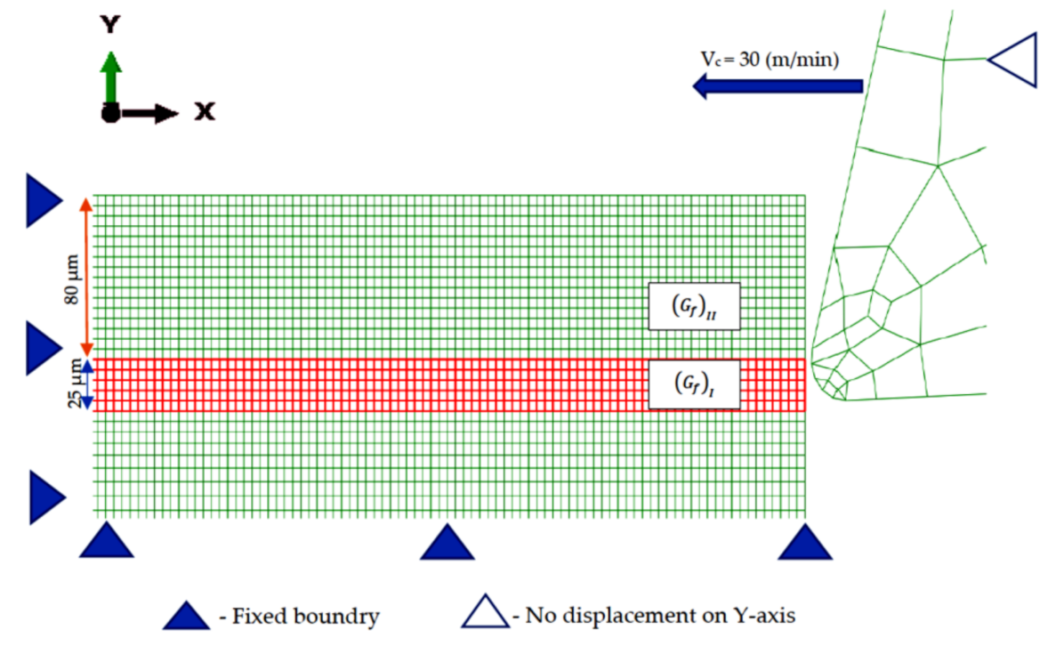
5. Finite Element Model

In this finite element model developed with Abaqus, the work piece is fixed in space and the tool moves over the workpiece with a prescribed velocity. A two-dimensional thermo-mechanical model with plain strain assumption is adopted for this work. An explicit algorithm with Lagrangian finite element formulation is considered for the simulation of orthogonal cutting process. The workpiece is modeled as an elastoplastic material, with the dimension of a rectangular block of 1.5 mm by 1 mm. The regions of interest in the work piece are modeled with an element size of 5 µm by 5 µm (that agrees with the size of grains) with square linear quadrilateral elements of type CPE4RT. The material properties adopted for the workpiece are given in

Table 5. Material properties considered for this study [34,35,36].

Material Properties	Ti6Al4V	Tungsten Carbide
$\mathrm{Density}, \rho$ (kg/m3)	4430	15,000
$\mathrm{Young}\text{’}\mathrm{s} \mathrm{modulus}, E$ (GPa)	113.8	800
$\mathrm{Poisson}\text{’}\mathrm{s} \mathrm{ratio} \nu$	0.342	0.2
$\mathrm{Expansion}, \alpha$ (K−1)	8.6 × 10−6	4.7 × 10−6
$\mathrm{Conductivity}, k$ (W/mK)	7.3	46
$\mathrm{Specific} \mathrm{heat}, cp$ (J/KgK)	580	203

. The interaction between tool and workpiece is modeled as Coulomb friction law with a friction coefficient of 0.2 [33].

Tungsten carbide is selected as tool material and the cutting tool is defined as an elastic material with the properties given in Table 5. The cutting conditions and tool geometry are the same as in the experiments and are given in Table 2. The tool and the workpiece basic geometry along with the mesh are kept constant for all the finite element models. Only the uncut chip thickness and the associated fracture energy regions dimensions are altered accordingly.

The boundary conditions and the basic geometry for the uncut chip thickness $h$ = 100 µm are illustrated in Figure 5. The predefined temperature field for both tool and workpiece is defined according to the parameters set chosen for simulation.

For this study, an energy-based failure criterion is adopted for FE modeling of orthogonal cutting simulation using Lagrangian formulation [37]. For chip separation criteria, a two-stage process is considered: damage or fracture initiation and fracture evolution. For damage initiation, Johnson–Cook damage model [23] is considered.

$$D=\mathsf{\Sigma } \frac{\Delta \epsilon }{{\epsilon }_f} ,$$

(7)

where $D$ is an internal state variable which links the ratio between the incremental plastic strain (∆ε) and the effective plastic strain to fracture $\left({\epsilon }_f\right)$. $D$ is a monotonically increasing function and the damage initiation occurs when D reaches the values of 1. The term ${\epsilon }_f$, takes the form.

$${\epsilon }_f=\left[d_1+d_2\exp d_3\left(\frac{p}{\overline{\sigma }}\right)\right]\left[1+d_{4}ln\left(\frac{\dot{\epsilon }}{{\dot{\epsilon }}_0}\right) \right]\left[1+d_5\left(\frac{T-T_{room}}{T_{melt}-T_{room}}\right)\right],$$

(8)

The material parameters $d_1,d_2,d_3$ indicates the fracture strain dependency to the triaxial stress, $d_4$ the strain-rate dependency and $d_5$ accounts for temperature softening these values are obtained through mechanical properties experiments. The JC failure model parameters adopted for Ti6Al4V are reported in

Table 6. Johnson–Cook failure parameters [33].

Material	${\mathit{d}}_1$	${\mathit{d}}_2$	${\mathit{d}}_3$	${\mathit{d}}_4$	${\mathit{d}}_5$
Ti6Al4V	−0.09	0.27	0.48	0.14	3.87

.

An energy-based fracture criterion is applied to the FE model for failure evolution. The failure evolution law is specified in terms of fracture energy dissipation $G_f$ [38]. $G_f$ is defined as the energy required to open a unit area of crack. After damage initiation instead of a stress–strain response, a stress-displacement response is followed. The fracture energy is defined as:

$$G_f={{\displaystyle \int }}_{{\epsilon }_f=0}^{{\epsilon }_f=1}L \sigma d\epsilon ={{\displaystyle \int }}_0^{u_{f=1}}\sigma du ,$$

(9)

where L is the characteristic length of the element (it depends on the element geometry) and $u$ is the equivalent plastic displacement at failure. Before damage initiation, $u=0$ and after damage initiation $u=L\epsilon$ [39].

From the concept of fracture mechanics, it is considered that during orthogonal cutting process two different values of fracture energies are considered as an input in Abaqus explicit code. In orthogonal cutting, the crack propagation is a combination of Mode I (opening mode) and Mode II (shearing mode). The Mode II will occur along shear plane accompanied by considerable shear deformation that are evident in region 1 and are given by fracture energy ($G_f$)_II. The ($G_f$)_I denotes the fracture energy of Mode I which is a tensile mode (opening mode normal to the plane of the fracture). The layer of chip is defined by region 1 and the tool passage layer is defined by region 2 [35,37,40], as shown in Figure 5. The thickness of the regions is given by the equation:

$$\begin{array}{c}Thickness of the region I=uncut chip thickness – cutting edge radius of the tool, \\ Thickness of the region II=cutting edge radius+one element\end{array}$$

(10)

The fracture energy is given by Equation (9) [27]:

$${\left(G_f\right)}_{I,II}=\left(\frac{1-{\nu }^2}{E}\right) {\left(K_c^2\right)}_{I,II}$$

(11)

where $K_c$ is fracture toughness and the value of $K_{Ic}$= 55 MPa√m [41], $E$ is the Young’s modulus and $\nu$ is Poisson’s ratio. The evolution of damage $D_f$ in chosen to be an exponential. When $D$ = 1 and $D_f$ = 0, damage is initiated, and the material fails when $D_f$ reaches 1.

In this paper a total of 48 finite element simulations has been performed by considering three sets of parameters for four different uncut chip thickness with each of the four constitutive models.

6. Numerical Results and Discussions

Initially, JC_1, JC-Hou_2, JC-Calalamz_3 and JC-MTANH_3 (i.e., the numerical simulation of JC-MTANH_3 is performed with set of parameters identified by Calamaz et al. [25] with $m_1$ from Hou et al. [30]) for uncut chip thickness of 60 µm are analyzed and compared with the experimental reference. Further they are investigated with different parameters sets of parameters with the three other uncut chip thickness (40 µm, 100 µm and 280 µm) considered in this study.

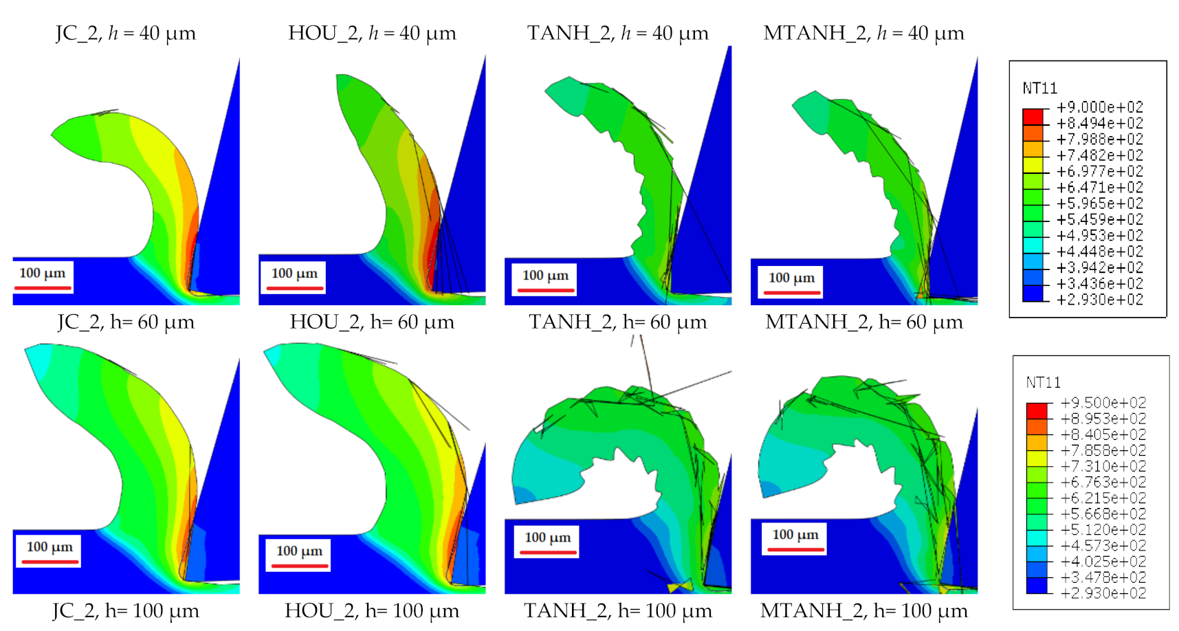
6.1. Comparison of Constitutive Models for Uncut Chip Thickness of 60 µm

The temperature distribution of JC_1, JC-Hou_2, JC-Calamaz_3 and JC-MTANH_3 chips are shown in Figure 6a–d. Heat transfer in the machining process takes place primarily in the shear zones, where the plastic work is converted into heat and the chip-tool interface where frictional heat is generated [36]. The maximum temperature observed in the secondary deformation zones is expected. Indeed, differences in temperature are seen between the simulated chips from these models. The temperature in the secondary deformation zone of chips produced by JC_1 and JC-HOU_2 is quite close and higher when compared with JC-Calamaz_3 and JC-MTANH_3. That can be explained by the level of stresses shown in Figure 1 and Figure 2.

The temperature in the numerically simulated chip from JC-MTANH_3 model is notably high when compared with JC-Calamaz_3 model. It is also important to note that in JC-Calamaz model the temperature distribution is somewhat uniform throughout the chip. In addition, highly deformed and elongated elements are observed in JC-Calamaz_3 and JC-MTANH_3. The contour plots of equivalent plastic strain for JC_1, JC-Hou_2, JC-Calalamz_3 and JC-MTANH_3 is shown in Figure 7a–d. In JC_1 and JC-Hou_2 models, high plastic strain is located in the chip side in contact with the tool rake face.

The plastic strain distribution of JC-Calamaz_3 and JC-MTANH_3 models show a sequence of two unequal segments with high strain localized areas and areas where the deformation is very low which confirms the serration in chip. The equivalent plastic strain contour of JC-MTANH_3 is similar to the JC-Calamaz_3 model. The only difference is that number of uncompleted serrations observed in the numerical chip simulated by the JC-MTANH_3 model is less when compared with the JC-Calamaz_3 model. This can be explained by the introduction of strain hardening term in the equation that alters the initial stress level of the JC-MTANH_3 model, when compared with the JC-Calamaz_3 model as shown in the stress strain evolution curve in Figure 1 and Figure 2. Equivalent plastic strain (PEEQ) is in the range of 1 to 2.5. PEEQ value may go up to 8 due to highly elongated elements highlighted in Figure 7c,d.

The morphology of the numerical chips of JC_1 and JC-Hou_2 is continuous, as expected but the numerical chip of JC-Calamaz_3 and JC-MTANH_3 is not continuous (slightly serrated chip) which is contrary to the experimental reference for this particular cutting condition. This can be explained by the fact that the JC-Calamaz and JC-MTANH_3 models and their parameters are optimized for cutting conditions considered by Calamaz et al. [25] that lead to serrated chips.

The RMS values of cutting force for JC_1 (108 N/mm) and JC-Hou_2 (110 N/mm) are nearly similar to the experimental reference. The cutting force values of JC-Calamaz_3 and JC-MTANH_3 are quite similar, but they are far below the experimental values. This can be explained by level of stresses at higher temperature as shown in Figure 2. The feed force values are slightly over estimated (within the range of 4 N/mm to 17 N/mm). The JC_1 and JC-Hou_2 produces chip thickness nearly same as experiment. But the JC-Calamaz_3 and JC-MTANH_3 produces slightly serrated chip. For qualitative analysis, a mean thickness value is calculated by taking the mean of peak and valley values of the serrated chips. This thickness is small when compared with experimental result. The RMS values of forces and chip thickness for $h$ = 60 µm are given in

Table 7. RMS cutting force (Fc), feed force (Ff), chip thickness ($h^{\prime }$ ) and ${\mathsf{\Delta }}_{\mathrm{x}}$ differences with the experimental forces of $h$ = 60 µm.

Uncut Chip Thickness (µm)	Models	Fc (N/mm)	Δ Fc(%)	Ff (N/mm)	Δ Ff(%)	${\mathit{h}}^{\prime }$ (µm)	${\mathsf{\Delta }}_{{\mathit{h}}^{’}}$ (%)
60	Experiment	112 ± 2	-	45 ± 1	-	80 ± 4
	JC_1	108	3	51	11	74	7
	JC_2	106	5	49	7	79	1
	JC_3	95	15	48	6	75	6
	JC-Hou_1	109	2	50	9	77	3
	JC-Hou_2	111	1*	47	4	81	1*
	JC-Hou_3	98	13	49	8	77	3
	JC-Calamaz_1	92	18	55	21	65	19
	JC-Calamaz_2	89	20	50	9	63	21
	JC-Calamaz_3	81	27	53	17	60	25
	JC-MTANH_1	92	18	59	30	71	10
	JC-MTANH_2	89	20	53	17	70	11
	JC-MTANH_3	82	26	53	17	64	20

Number*—the difference is in the uncertainty range of the measurement.

.

To conclude on the results of the comparison on the four phenomenological constitutive models for the above cutting condition, the predictive finite element model with JC_1 and JC-Hou_2 models can accurately predict forces, chip morphology and chip thickness. The results from JC-MTANH model are nearly the same as from the JC-Calamaz model, even though JC-MTANH model includes temperature dependent strain hardening factor.

6.2. Influence of Parameters Sets for Different Uncut Chip Thickness

This part will focus on the combined influence of parameters sets and constitutive models on the results, which is further extended to the different uncut chip thickness considered in this study. It is important to note that for Ti6Al4V there is large availability of parameters sets in the literature. The constitutive models are fitted even on the physical parameters which can be seen as problematic. Determining the most suitable parameters sets is always a concerning point in numerical simulation of machining process. In this context three sets of parameters are considered as given in Table 1. To validate the influence of the choice of the parameters and effect of uncut chip thickness on constitutive models, only parameters sets are interchanged in the constitutive models for 4 uncut chip thickness (i.e., 4 models are employed with 3 sets of parameters for 4 different uncut chip thickness making a total of 48 (4 × 3 × 4) simulations).

6.2.1. Forces

Cutting and feed forces are generated using these models for the uncut chip thickness of 40 µm. The RMS value of cutting force calculated from JC and JC-Hou with set 1 and set 2 parameters are quite close around 86 N/mm, but with set 3 parameters significant differences are observed. This can be explained by the fact that the set 3 parameters are identified by Calamaz et al. [17] for a particular cutting condition. Comparing with the two other constitutive models, JC-Calamaz and JC-MTANH, with any set of parameters predicts cutting force value well below the experimentally calculated values and includes oscillation in the force evolution. This can be explained by the presence of hyperbolic function in JC-Calamaz and JC-MTANH models.

The RMS value of feed force calculated from the JC and JC-Hou models with set 1 and set 2 parameters are in variation of +9 N/mm to +25 N/mm when compared with experimental result. The feed force calculated from JC-Calamaz_3 and JC-MTANH_3 is higher when compared with JC and JC-Hou. The RMS values cutting force and feed force are given in

Table 8. RMS cutting force (Fc), feed force (Ff), chip thickness ($h^{\prime }$ ) and ${\mathsf{\Delta }}_{\mathrm{x}}$ differences with the experimental forces of $h$ = 40 µm.

Uncut Chip Thickness (µm)	Models	Fc (N/mm)	ΔFc (%)	Ff (N/mm)	ΔFf (%)	${\mathit{h}}^{\prime }$ (µm)	${\mathsf{\Delta }}_{{\mathit{h}}^{\prime }}$ (%)
40	Experiment	86 ± 2	-	41 ± 1	-	59 ± 5	-
	JC_1	87	1*	48	14	48	10
	JC_2	82	3	46	9	50	7
	JC_3	78	7	52	24	56	3*
	JC-Hou_1	87	1*	50	20	49	9
	JC-Hou_2	86	-	47	12	48	10
	JC-Hou_3	80	4	53	25	54	5*
	JC-Calamaz_1	68	19	54	29	43	20
	JC-Calamaz_2	61	27	53	26	41	24
	JC-Calamaz_3	63	26	59	40	47	16
	JC-MTANH_1	60	28	47	12	42	18
	JC-MTANH_2	61	27	52	24	40	26
	JC-MTANH_3	68	19	68	62	46	12

Number*—the difference is in the uncertainty range of the measurement.

.

When the uncut chip thickness increases, the RMS value of cutting force increases for all the constitutive models with any sets of parameters in the same pattern as for the uncut chip thickness of 40 µm. Indeed, the RMS values of cutting force for JC and JC-Hou with set 1 and set 2 parameters are quite close, but with set 3 parameters differences are quite high when compared with experiments. The JC-Calamaz and JC-MTANH with any set of parameters give lower cutting force values when compared with the two other models. The RMS values of forces for $h$ = 100 µm and 280 µm are given in

Table 9. RMS cutting force (Fc), feed force (Ff), chip thickness ($h^{\prime }$ ) and ${\mathsf{\Delta }}_{\mathrm{x}}$ differences with the experimental forces of $h$ = 100 µm.

Uncut Chip Thickness (µm)	Models	Fc (N/mm)	ΔFc (%)	Ff (N/mm)	ΔFf (%)	${\mathit{h}}^{\prime }$ (µm)	${\mathsf{\Delta }}_{{\mathit{h}}^{\prime }}$ (%)
100	Experiment	173 ± 2	-	51 ± 1	-	135 ± 6	-
	JC_1	168	2	44	12	132	2*
	JC_2	160	6	44	12	130	4*
	JC_3	142	17	45	10	138	2*
	JC-Hou_1	171	1*	44	12	132	2*
	JC-Hou_2	164	4	44	12	132	2*
	JC-Hou_3	146	15	47	6	142	5*
	JC-Calamaz_1	138	19	65	25	126	2
	JC-Calamaz_2	132	23	69	33	122	3
	JC-Calamaz_3	120	30	69	33	120	3
	JC-MTANH_1	129	25	57	10	132	2*
	JC-MTANH_2	130	24	58	11	132	2*
	JC-MTANH_3	125	27	73	48	118	3

Number*—the difference is in the uncertainty range of the measurement.

and

Table 10. RMS cutting force (Fc), feed force (Ff), chip thickness ($h^{\prime }$) and ${\mathsf{\Delta }}_{\mathrm{x}}$ differences with the experimental forces of $h$ = 280 µm.

Uncut Chip Thickness (µm)	Models	Fc (N/mm)	ΔFc (%)	Ff (N/mm)	ΔFf (%)	${\mathit{h}}^{\prime }$ (µm)	${\mathsf{\Delta }}_{{\mathit{h}}^{\prime }}$ (%)
280	Experiment	387 ± 2	-	77 ± 4	-	-	-
	JC_1	393	1	39	47	362	-
	JC_2	369	4	41	44	350	-
	JC_3	323	16	43	41	342	-
	JC-Hou_1	407	5	37	50	364	-
	JC-Hou_2	378	2	41	44	345	-
	JC-Hou_3	330	14	43	41	344	-
	JC-Calamaz_1	270	30	60	18	*	-
	JC-Calamaz_2	274	29	51	30	*	-
	JC-Calamaz_3	256	33	96	19	*	-
	JC-MTANH_1	264	31	56	23	*	-
	JC-MTANH_2	275	29	53	27	*	-
	JC-MTANH_3	253	34	75	2*	*	-

Number*—the difference is in the uncertainty range of the measurement. * these chips are fully developed serrated chips and the corresponding measurements are given in Table 11.

.

The RMS values of feed force for uncut chip thickness of 40 µm and 60 µm is overestimated by all the four models with any set of parameters. However, for uncut chip thickness of 100 µm and 280 µm the RMS feed force value from JC and JC-Hou with any set of parameters is underestimated. On the contrary, JC-Calamaz and JC-MTANH with set 3 parameters overestimate the value of feed force for uncut chip thickness of 100 µm and 280 µm.

From this investigation, the force values generated by set 2 parameters with the four constitutive models show improvement towards the prediction of cutting force and feed force near to the experimental value.

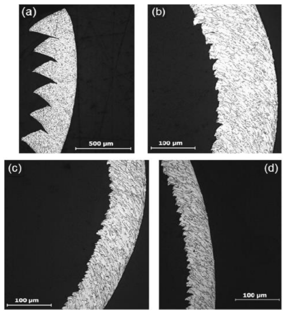
6.2.2. Predicted Chip Morphology

The chip morphologies for uncut chip thickness of 40 µm, 60 µm, 100 µm and 280 µm are analyzed in this section. Continuous chips are produced by JC and JC-Hou for any uncut chip thickness and with any sets of parameters. Whereas the JC-Calamaz and JC-MTANH model with any set of parameters for uncut chip thickness of 40 µm, 60 µm and 100 µm produces slightly serrated chip. This serration becomes more pronounced with increase of uncut chip thickness to 280 µm.

Initially the temperature contours of uncut chip thickness of 280 µm are analyzed and are plotted in Figure 8. The temperature rise in the secondary shear zone is evident for all models with any set of parameters. When the uncut chip thickness increases the temperature in the secondary deformation zone also increases. It is also observed that the large increase of temperature in the primary shear zone leading to the formation of the adiabatic shear band is clearly noticed for 280 µm with JC-Calamaz and JC-MTANH. In addition to above discussion the evolution of cutting force clearly depicts the oscillation in the curve which confirms the presence of serrated chip. The JC and JC-Hou models produce continuous chip with maximum temperature value localized along the tool-chip interface with steady state evolution of forces.

It is also observed that temperature is higher and quite close for JC and JC-Hou models with parameters sets 1 and 2. But with set 3 parameters the temperature is comparatively lower. The JC-Calamaz and JC-MTANH models follow the same trend: with set 1 and set 2 parameters, the temperature is high, and with set 3 parameters, the temperature is low. Nevertheless, the temperature is notably higher for JC and JC-Hou models regardless of the parameters sets.

For the three other cutting conditions ($h$ = 40 µm, 60 µm and 100 µm), the temperature is higher and quite close for JC and JC-Hou models with set 1 and set 2 parameters, whereas with set 3 parameters, the temperature is less. This follows the same trend as for $h=2$80 µm. Continuous chips are observed in all the cases, and it is obvious that temperature rises mainly in the deformation zone of chip region, with maximum values localized along the tool-chip interface.

The JC-Calamaz and JC-MTANH model for $h$ = 40 µm and 60 µm the temperature distribution is relatively homogenous in the chip for any set of parameters and the maximum temperature is not clearly observed in the secondary deformation zone. When the uncut chip thickness increases to 100 µm, the temperature variations are observed with maximum temperature in the secondary deformation zone. This might be due to the incorporation of hyperbolic tangent function in the behavior law that alters the stress level and influences the temperature.

The adiabatic shear bands are not clearly noticed for this cutting condition. Nevertheless, the chips produced by these two constitutive models are slightly serrated and the serration is further confirmed by investigating the equivalent plastic strain contour. It is also worth noting that JC and JC-Hou models produce a continuous chip with less distorted or elongated elements in the chip region whereas with the JC-Calamaz and JC-MTANH models, highly elongated and distorted elements are clearly visible. This could possibly influence the results to some extent.

Overall, when the uncut chip thickness increases, the temperature in the secondary deformation zone also increases. This is because when h, increases the tool experiences more cutting resistance resulting in an increased temperature. Some improvements in the forces and temperature values are seen from the results produced by all the models with set 2 parameters. The temperature contours of $h$ = 40 µm, 60 µm and 100 µm with set 2 parameters for the four constitutive models are given in Figure 9.

Equivalent plastic strain contours are analyzed to clearly understand the chip morphologies. For continuous chips, the equivalent plastic strain (PEEQ) lies in the range of 1 to 3 and for serrated chip the equivalent plastic strain is approximately in the range of 1–5. However, in some cases PEEQ reaches the value of 10 or even more where elements are highly distorted or elongated.

For all the continuous chips produced by the JC and JC-Hou models, high plastic strain is observed at the chip side in contact with the tool rake face. For slightly serrated chips from JC-Calamaz and JC-MTANH two unequal segments with high strain localized areas and areas with low deformation is observed. This further confirms the presence of serration in the chips.

The saw tooth is clearly observed for $h$ = 280 µm and are presented in Figure 10. The chip thickness values of the continuous chips from JC and JC-Hou for $h$ = 40 µm, 60 µm and 100 µm with any set of parameters are within the deviation range of 1% to 10%. In some cases, a thinning of chips is observed with the increase of feed force.

For a qualitative comparison, a mean thickness value of the serrated chips produced by JC-Calamaz and JC-MTANH for $h$ = 40 µm, 60 µm and 100 µm is measured and is compared with the experimental reference. The mean chip thickness value of the serrated chips from JC-Calamaz and JC-MTANH models with any set of parameters is less when compared with chip thickness of continuous chips produced by JC and JC-Hou. The chip thickness values are summarized in Table 4, Table 5, Table 6 and Table 7. The chip measurement of full serrated chips produced by JC-Calamaz and JC-MTANH for $h$ = 280 µm are given in

Table 11. Numerical saw-toothed chip measurement of tooth length, L, the tooth height,$H$, the valley, $C$ and the standard deviation of the length x for $h$ = 280 µm, ${\sigma }_x$.

Models	$\mathit{L} (\mathsf{\mu }\mathbf{m})$	${\mathit{\sigma }}_{\mathit{L}} (\mathsf{\mu }\mathbf{m})$	$\mathit{H} (\mathsf{\mu }\mathbf{m})$	${\mathit{\sigma }}_{\mathit{H}} (\mathsf{\mu }\mathbf{m})$	C (µm)	${\mathit{\sigma }}_{\mathit{C}} (\mathsf{\mu }\mathbf{m})$
Experiment	206	17	288	14	157	21
JC-Calamaz_1	171	12	316	16	108	26
JC-Calamaz_2	188	16	302	26	82	17
JC-Calamaz_3	168	9	288	5	104	18
JC-MTANH_1	178	11	312	12	112	21
JC-MTANH_2	180	19	306	28	101	8
JC-MTANH_3	166	7	287	7	96	16

.

The parameters used to characterize chip serration are given in Figure 10. The length of the tooth is represented by $L$. The maximum tooth height or peak and the valley from the base of the chip are represented by $H$ and $C,$ respectively.

7. Discussion

For uncut chip thickness h = 40 µm, 60 µm and 100 µm, the RMS values of cutting force from JC and JC-Hou models with set 1 and set 2 parameters are very close to the experimental values within the range of ±5% and feed forces are in the range of ±20%. With set 3 parameters, the cutting forces values are notable less with a difference of 15% when compared with experimental reference, whereas the feed force are in the same range. The JC-Calamaz and JC-MTANH models with any set of parameters underestimate the cutting force value (with a difference of 25%) and overestimate feed force value (in the deviation range of 25%).

For the case of $h$= 280 µm, the trend is somewhat different. The JC and JC-Hou models with sets 1 and 2 parameters cutting force are in the same range at ±5%, but underestimate feed force (with a difference of 50%). The cutting and feed force values are underestimated (with a difference of 35%) by JC-Calamaz and JC-MTANH models with set 1 and set 2 parameters when compared with experimental results. Based on the above discussions, the cutting force values predicted by JC-Calamaz and JC-MTANH models with any sets of parameters are very low when compared with experimental force values. Indeed, the metallurgical state and operating conditions of Ti6Al4V considered by Calamaz et al. [25] is unknown and may be different from the Ti6Al4V employed in experiments. This might influence the force calculation.

The temperature in the secondary deformation zone increases while uncut chip thickness increases, and a direct link was observed between temperature and cutting force value for all the cases. The comparison of simulated chips with the experimental chips shows that JC and JC-Hou constitutive models with any sets of the parameters for h = 40 µm, 60 µm and 100 µm produce continuous chip as the experimental reference.

Considering uncut chip thickness $h$ = 280 µm, the chip morphology observed from the experiments is a saw-toothed chip, but the JC and JC-Hou models with any set of parameters give continuous chip. This is because in JC and JC-Hou law flow stress increases with increasing strain regardless of temperature. In addition, Guo et al. [42] demonstrated that these models lack in predicting the adiabatic phenomenon responsible for serrated chip formation observed during machining of these alloys.

On the contrary, the JC-Calamaz and JC-MTANH models produce slightly serrated chips for all cutting conditions and with any set of parameters considered in this study. This serration of chip is more prominent with increase of uncut chip thickness.

From the above discussions, JC-Hou with set 2 parameters predicts cutting force and feed force values very close to the experiments for all uncut chip thicknesses considered in this study. This model can predict the chip morphologies for small uncut chip thickness i.e., $h$ = 40 µm, 60 µm and 100 µm but, fails to predict the chip morphology for h = 280 µm. This is because this model does not include an important behavior of Ti6Al4V when machined: the adiabatic and strain softening phenomenon observed. Even though the JC-Calamaz and JC-MTANH models include strain softening phenomenon and temperature dependent strain hardening factor, the chips produced by these models are all serrated for any uncut chip thickness, although this is not the case with the experimental chips.

The experimental results from Ducobu et al. [31] highlight that the chip morphology at a constant cutting speed of 30 m/min is influenced by the uncut chip thickness. The increase in chip thickness leads to the accumulation of heat in the primary shear zone which promotes the serrated chip. The FE simulation and constitutive models fails to predict the transition from continuous chip to serrated chip for any set of parameters and the cutting conditions considered in this study.

The JC-MTANH model proposed in this work which incorporates temperature dependent strain hardening and hyperbolic tangent law together does not show a notable improvement in predicting the forces and chip thickness values. Meanwhile, JC law with temperature dependent hardening factor can significantly improves the prediction of forces and chip thickness.

Overall, the main objective of this work is to employ the exact same FE model for different cutting condition to predict forces and chip morphologies. These models work well for some cutting conditions and fails for other cutting condition. Consequently, for the cutting conditions considered in this work, all the models examined in this study fail to capture the transition of continuous chip to serrated chip. The transition from continuous chip to serrated chip and the influence of strain softening phenomenon and their temperature dependency is still a valid question. In addition, identification of the right parameters sets is of prime importance in predicting the forces and chip thickness through numerical simulation of cutting process.

8. Conclusions

In this research work, comparison of constitutive models and the influence of parameters sets on different uncut chip thickness was performed through finite element analysis of orthogonal cutting of Ti6Al4V. In the meantime, a reconstructed constitutive model is proposed. The forces and chip morphologies from FE simulations are compared with experimental references to highlight the differences. The following conclusions are drawn from this study:

• A direct link is observed between temperature and cutting force values.
• JC-Hou with parameters set 2 predictors equivalent cutting force as experimental reference for all uncut chip thickness considered in this study. It also predicts the chip morphology of h = 40 µm, 60 µm and 100 µm (continuous chips) but fails at $h$ = 280 µm (serrated chip).
• JC-MTANH model does not show a significant improvement in the prediction of forces and chip morphologies.
• JC-Calamaz model predicts the chip morphology at $h$ = 280 µm but fails to predict chip morphologies of smaller uncut chip thicknesses and the force values.
• JC-Calamaz model with set 1 and set 2 parameters shows a significant improvement in the force calculation.

References

1. Lütjering, G.; Williams, J.C. Titanium (Engineering Materials and Processes); Springer: Berlin/Heidelberg, Germany, 2013. [Google Scholar]
2. Boyer, R. Materials Properties Handbook; ASM International: Materials Park, OH, USA, 1994. [Google Scholar]
3. Bridges, P.J.; Magnus, B. Manufacture of Titanium Alloy Components for Aerospace and Military Applications; Cost Effective Application of Titanium Alloys in Military Platforms; RTO-MP-069(II); Research and Technology Organization: France, 2002. [Google Scholar]
4. Arrazola, P.J.; Özel, T.; Umbrello, D.; Davies, M.; Jawahir, I.S. Recent advances in modelling of metal machining processes. Cirp Ann. Manuf. Technol. 2013, 62, 695–718. [Google Scholar] [CrossRef]
5. Komanduri, R. Some clarifications on the mechanics of chip formation when machining titanium alloys. Wear 1982, 76, 15–34. [Google Scholar] [CrossRef]
6. Komvopoulos, K.; Erpenbeck, S.A. Finite Element Modeling of Orthogonal Metal Cutting. J. Eng. Ind. 1991, 113, 253–267. [Google Scholar] [CrossRef]
7. Davim, J.P. (Ed.) Finite Element Method in Machining Process; Springer: Berlin/Heidelberg, Germany, 2013. [Google Scholar]
8. Ducobu, F.; Rivière-Lorphèvre, E.; Filippi, E. Numerical contribution to the comprehension of saw-toothed Ti6Al4V chip formation in orthogonal cutting. Int. J. Mech. Sci. 2014, 81, 77–87. [Google Scholar] [CrossRef]
9. Pantalé, O.; Bacaria, J.-L.; Dalverny, O.; Rakotomalala, R.; Caperaa, S. 2D and 3D numerical models of metal cutting with damage effects. Comput. Methods Appl. Mech. Eng. 2004, 193, 4383–4399. [Google Scholar] [CrossRef] [Green Version]
10. Arrazola, P.J.; Özel, T. Investigations on the effects of friction modeling in finite element simulation of machining. Int. J. Mech. Sci. 2010, 52, 31–42. [Google Scholar] [CrossRef]
11. Subbiah, S.; Melkote, S.N. Effect of finite edge radius on ductile fracture ahead of the cutting tool edge in micro-cutting of Al2024-T3. Mater. Sci. Eng. 2008, 474, 283–300. [Google Scholar] [CrossRef]
12. Ohbuchi, Y.; Obikawa, T. Finite Element Modeling of Chip Formation in the Domain of Negative Rake Angle Cutting. J. Eng. Mater. Technol. 2003, 125, 324–332. [Google Scholar] [CrossRef]
13. Umbrello, D. Finite element simulation of conventional and high speed machining of Ti6Al4V alloy. J. Mater. Process. Technol. 2008, 196, 79–87. [Google Scholar] [CrossRef]
14. Ducobu, F.; Arrazola, P.; Rivière-Lorphèvre, E.; Filippi, E. Finite Element Prediction of the Tool Wear Influence in Ti6Al4V Machining. Procedia Cirp 2015, 31, 124–129. [Google Scholar] [CrossRef] [Green Version]
15. Ducobu, F.; Rivière-Lorphèvre, E.; Filippi, E. Application of the Coupled Eulerian-Lagrangian (CEL) method to the modeling of orthogonal cutting. Eur. J. Mech. A/Solids 2016, 59, 58–66. [Google Scholar] [CrossRef]
16. Ducobu, F.; Rivière-Lorphèvre, E.; Filippi, E. Finite element modelling of 3D orthogonal cutting experimental tests with the Coupled Eulerian-Lagrangian (CEL) formulation. Finite Elem. Anal. Des. 2017, 134, 27–50. [Google Scholar] [CrossRef]
17. Vaz, M., Jr. Modelling and Simulation of Machining Processes. Arch. Comput. Methods Eng. 2010, 14, 173–204. [Google Scholar] [CrossRef]
18. Cotterell, M.; Ares, E.; Yanes, J.B.; Lopez, F.R.J.; Hernandez, P.P.; Peláez, G. Temperature and Strain Measurement during Chip Formation in Orthogonal Cutting Conditions Applied to Ti-6Al-4V. Procedia Eng. 2013, 63, 922–930. [Google Scholar] [CrossRef] [Green Version]
19. Ducobu, F.; Rivière-Lorphèvre, E.; Filippi, E. Influence of the Material Behavior Law and Damage Value on the 9Results of an Orthogonal Cutting Finite Element Model of Ti6Al4V. Procedia Cirp 2013, 8, 379–384. [Google Scholar] [CrossRef] [Green Version]
20. Ducobu, F.; Rivière-Lorphèvre, E.; Filippi, E. Comparison of several behaviour laws intended to produce a realistic Ti6Al4V chip by finite elements modelling. Key Eng. Mater. 2015, 651-653, 1197–1203. [Google Scholar] [CrossRef]
21. Johnson, G.R.; Cook, W.H. A constitutive model and data for metals subjected to large strains, high strain rates and high temperatures. In Proceedings of the Seventh International Symposium on Ballistics, Hague, The Netherlands, 19–21 April 1983; pp. 541–547. [Google Scholar]
22. Johnson, G.R.; Cook, W.H. Fracture characteristics of three metals subjected to various strains, strain rates, temperatures and pressures. Eng. Fract. Mech. 1985, 21, 31–48. [Google Scholar] [CrossRef]
23. George, T. Classic Split-Hopkinson Pressure Bar Testing. In Mechanical Testing and Evaluation; ASM Handbook; Kuhn, H., Medlin, D., Eds.; ASM International: Materials Park, OH, USA, 2000; Volume 8, pp. 462–476. [Google Scholar]
24. Sima, M.; Özel, T. Modified material constitutive models for serrated chip formation simulations and experimental validation in machining of titanium alloy Ti–6Al–4V. Int. J. Mach. Tools Manuf. 2010, 50, 943–960. [Google Scholar] [CrossRef]
25. Calamaz, M.; Coupard, D.; Girot, F. A new material model for 2D numerical simulation of serrated chip formation when machining titanium alloy Ti–6Al–4V. Int. J. Mach. Tools Manuf. 2008, 48, 275–288. [Google Scholar] [CrossRef] [Green Version]
26. Umbrello, D.; M’Saoubi, R.; Outeiro, J.C. The influence of Johnson-Cook material constants on finite element simulation of machining of AISI 316L steel. Int. J. Mach. Tools Manuf. 2007, 47, 462–470. [Google Scholar] [CrossRef]
27. Karpat, Y. A modified material model for the finite element simulation of machining titanium Alloyti-6Al-4 V. Mach. Sci. Technol. 2010, 14, 390–410. [Google Scholar] [CrossRef] [Green Version]
28. Ducobu, F.; Rivière-Lorphèvre, E.; Filippi, E. On the importance of the choice of the parameters of the Johnson-Cook constitutive model and their influence on the results of a Ti6Al4V orthogonal cutting model. Int. J. Mech. Sci. 2017, 122, 143–155. [Google Scholar] [CrossRef]
29. Kugalur-Palanisamy, N.; Rivière-Lorphèvre, E.; Ducobu, F.; Arrazola, P.-J. Influence of the Choice of the Parameters on Constitutive Models and their Effects on the Results of Ti6Al4V Orthogonal Cutting Simulation. Procedia Manuf. 2020, 47, 458–465. [Google Scholar] [CrossRef]
30. Hou, X.; Liu, Z.; Wang, B.; Lv, W.; Liang, X.; Hua, Y. Stress-Strain Curves and Modified Material Constitutive Model for Ti-6Al-4V over the Wide Ranges of Strain Rate and Temperature. Materials 2018, 11, 938. [Google Scholar] [CrossRef] [Green Version]
31. Seo, S.; Min, O.; Yang, H. Constitutive equation for Ti–6Al–4V at high temperatures measured using the SHPB technique. Int. J. Impact. Eng. 2005, 31, 735–754. [Google Scholar] [CrossRef]
32. Ducobu, F.; Rivière-Lorphèvre, E.; Filippi, E. Experimental contribution to the study of the Ti6Al4V chip formation in orthogonal cutting on a milling machine. Int. J. Mater. 2014, 8, 455–468. [Google Scholar] [CrossRef]
33. Melkote, S.N.; Grzesik, W.; Outeiro, J.; Rech, J.; Schulze, V.; Attia, H.; Arrazola, P.-J.; M’Saoubi, R.; Saldana, C. Advances in material and friction data for modelling of metal machining. Cirp Ann. 2017, 66, 731–754. [Google Scholar] [CrossRef] [Green Version]
34. Leseur, D. Experimental Investigations of Material Models for Ti-6A1-4V and 2024-T3; Lawrence Livermore National Lab.: Livermore, CA, USA, 1999. [Google Scholar] [CrossRef] [Green Version]
35. Bouchnak, T.B. Etude du Comportement en Sollicitations Extremes et de L’usinabilité d’un Nouvel Alliage de Titane Aéronautique: Le Ti555-3. Ph.D. Thesis, ENSAM, Paris, France, 2010. [Google Scholar]
36. Sun, J.; Guo, Y.B. Material flow stress and failure in multiscale machining titanium alloy Ti-6Al-4V. Int. J. Adv. Manuf. 2009, 41, 651–659. [Google Scholar]
37. Mabrouki, T.; Girardin, F.; Asad, M.; Rigal, J.-F. Numerical and experimental study of dry cutting for an aeronautic aluminium alloy (A2024-T351). Int. J. Mach. Tools Manuf. 2008, 48, 1187–1197. [Google Scholar] [CrossRef]
38. Kay, G. Failure Modeling of Titanium-6Al-4V and 2024-T3 Aluminum with the Johnson-Cook Material Model; Lawrence Livermore National Lab.: Livermore, CA, USA, 2002. [Google Scholar]
39. Simulia. Abaqus Analysis User’s Manual 6.14; Simulia: Johnston, RI, USA, 2014. [Google Scholar]
40. Zhang, Y.; Mabrouki, T.; Nelias, D.; Gong, Y. FE-model for Titanium alloy (Ti-6Al-4V) cutting based on the identification of limiting shear stress at tool-chip interface. Int. J. Mater. Form. 2011, 4, 11–23. [Google Scholar] [CrossRef]
41. Henry, S.D.; Dragolich, K.S.; Dimatteo, N.D. Fatigue Data Book: Light Structural Alloys; ASM International: Materials Park, OH, USA, 1995. [Google Scholar]
42. Guo, Y.B. Dynamic material behavior modelling using internal state variable plasticity and its application in hard machining simulations. J. Manuf. Sci. Eng. 2006, 128, 749–756. [Google Scholar] [CrossRef]
Figure 1. Stress-strain curves of JC, JC-Hou, JC-Calamaz and JC-MTANH at (a) T = 573 K and ε ˙ 0 = 10,000 s−1 and (b) at T = 973 K and ε ˙ 0 = 10,000 s−1.
Jmmp 05 00056 g001
Figure 2. Stress-strain curves of JC, JC-Hou, JC-Calamaz and JC-MTANH for 3 sets of parameters at T = 973 K and ε ˙ 0 = 10,000 s−1.
Jmmp 05 00056 g002
Figure 3. Cutting configuration on the milling machine [32].
Jmmp 05 00056 g003
Figure 4. Experimental chips (a) 280 µm, (b) 100 µm, (c) 60 µm and (d) 40 µm [32].
Jmmp 05 00056 g004
Figure 5. Finite element model for the uncut chip thickness of h   = 100 µm with relevant information’s on geometry, mesh, boundary condition and fracture energy concept.
Jmmp 05 00056 g005
Figure 6. Temperature contour (in K) of (a) JC_1, (b) JC_Hou_2, (c) JC-Calamaz_3 and (d) JC-MTANH_3 for h = 60 µm at 850 μs of cutting time.
Jmmp 05 00056 g006
Figure 7. PEEQ contour (a) JC_1, (b) JC_Hou_2, (c) JC-Calalamz_3 and (d) JC-MTANH_3 for h = 60 µm at 850 μs of cutting time.
Jmmp 05 00056 g007
Figure 8. Temperature contour (in K) for uncut chip thickness of 280 µm.
Jmmp 05 00056 g008aJmmp 05 00056 g008b
Figure 9. Temperature contour (in K) of four constitutive models with set 2 parameters for uncut chip thickness of 40 µm, 60 µm and 100 µm.
Jmmp 05 00056 g009aJmmp 05 00056 g009b
Figure 10. Equivalent plastic strain contour for uncut chip thickness of 280 µm.
Jmmp 05 00056 g010