Abstract
A model Numerical Control (NC) machine tool dynamic compliance is analyzed, including the influence of its mechanical structure and position control feed drive algorithms. The dynamic model of the machine tool is divided into two main parts, which are closest to the machining process. First, the milling head assembly group is presented as a system of one mass oscillating in a 2D plane and 3D space. Second, the motion axes assembly group, XY cross table with linear feed drive, is presented. A square dimension matrix of the total dynamic compliance is evaluated within the feed drive control system included. Partial elements of the mechanical structure dynamic compliance matrix of the general dimension are contained in the total dynamic compliance matrix.
1. Introduction
Chatter in machining represents a key limiting factor for achieving higher machining productivity. Increased vibration during machining results in higher spindle load, lower cutting tool lifetime, and deteriorated workpiece surface quality. The main sources of chatter result from machine tool and workpiece dynamic properties and the process force interaction between the cutting tool and the workpiece.
Typically, attention in modelling and predicting the machining stability focuses primarily on machine tool structural dynamics. In most cases, a simplified oscillator model composed of a mass-spring-damper, which is described by a second order transfer function, is considered as a representation of machine tool dynamic properties [1,2,3]. Another possible approach is a 2D planar model with mass oscillation in two degrees of freedom [4]. In complex tasks, Finite Element Method (FEM) is used for modelling and researching machine tool dynamics.
On the contrary, dynamic compliance of feed drive control and its impact on machining stability is the focus of research in only a few works [5,6]. Machining stability taking into account a simple proportional-derivative (PD) controller is demonstrated by Lehotzky [7]. The impact of cascade control feed drive parameters of motion axes with linear motors on machining stability is presented by Beudaert [8]. In this work, a simplified two-mass model of the mechanical axis system including the cutting force model is used. The impact of the feed drive control tuning on the process stability limit is demonstrated. Franco [9] performs experimental validation of the impact of feed drive control parameters using a test bench with linear motors and demonstrates performance improvement of chatter stability limits. The experimental equipment consists of a single axis and a two-mass vibrating system with appropriately selected stiffness and damping values. An analysis of machining stability limits on a mid-sized lathe with a ball-screw-driven X-axis is presented in [4] with application on the mid-sized lathe and Franco [10] in the double motor preloaded pinion and rack case. Recently, Beudaert presented a new feed drive controller tuning strategy enhancing machining stability in [11].
To determine the size of the limit chip width according to the classical theory [1], it is necessary to find a frequency range, where the real part of the machine tool dynamic compliance reaches its negative minimum. According to this process, the critical depth of cut as a dependency of the frequency and the cutting force coefficient is expressed by Equation (1). A graphical indication of the critical chip thickness (the limits of stability by the Nyquist diagram) is introduced in [12], which has become a standard (e.g., Altintas [13] or Smith [14]). Here, however, only simplified second order dynamic models are considered. Representation of the critical depth of cut dependency on the spindle speed is provided by the stability lobe diagram (SLD). The calculation procedure for getting the SLD is introduced in detail in, e.g., [1,2] or [15].
Weck [16] presents chatter-describing models with the force input signal. This paper works consistently with the setpoint chip thickness as an input signal. Some works present a concept of complex cutting force coefficients in detail Drobílek [17]. This approach is based on inner and outer cutting force modulation. However, validation of this principle for its use in the machining stability theory was not satisfactorily proved.
In this paper, a model of the directional dynamic properties of a CNC vertical machining center, including the feed drive control, is developed and used for the analysis of the impact of feed drive control setting on the machining stability limits. The machining center is equipped with linear motors on the XY cross table. The model of machine tool dynamics is considered as a sum of the spindle and XY cross table parts, including the X and Y axis feed drive control. The schematics of the feedback regenerative principle of real chip thickness resulting from the interaction of machine tool structural and control dynamics, expressed by the overall compliance , with cutting process, expressed by cutting force coefficient , chip thickness , and as the additional transfer function, expressing the dependency of on process parameters [18], is illustrated in Figure 1. The input to the feedback scheme is setpoint chip thickness.
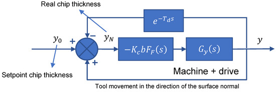
Figure 1.
Feedback regenerative principle for calculating real chip thickness.
2. Proposed Methodology
The machine tool (Figure 2) dynamic model is composed of two parts, representing the Z-axis vertical column with the spindle unit and XY cross table. The Z-axis drive is equipped with a linear motor, while the XY cross table is equipped with linear motors as well. The spindle unit is described by the transfer function and the XY cross table is represented by the transfer function (Figure 3).
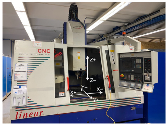
Figure 2.
Vertical milling center MCFV 5050 LN (TAJMAC-ZPS, Zlín, Czechia).
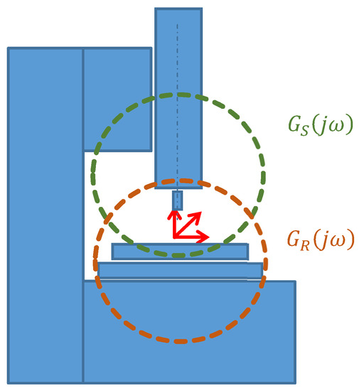
Figure 3.
Scheme of machine tool structural parts modeled by and dynamic compliance.
The XY cross table dynamic system can be divided into the mechanical structure part described by the transfer function and the feed drive control part described by the transfer function. The overall dynamic compliance is expressed as a sum of the structural and control parts, as indicated by Equation (2). The overall is evaluated in the XY plane, thus enabling evaluation of the most critical direction of machine tool dynamic behavior with respect to the directional dynamic compliance. At the same time, is used to evaluate the impact of X and Y motion axis feed drive control parameters on the stable cut limits. The procedure of obtaining the directional dynamic compliance of the machine tool mechanical structure at a spindle and XY cross table is described in the following chapters.
where:
3. Spindle Dynamic Compliance
A model of directional dynamic compliance of the spindle unit is developed based on measurements. Direct dynamic compliance measurements were executed in parallel with the XY cross table with the use of an electric-dynamic vibration source and one-axis accelerometer. This process is deemed more reliable compared to the use of a modal hammer. The measurements were taken starting in the negative direction of axis Y and proceeded in the 1° step in the clockwise direction (Figure 4). Every single measurement consisted of the force excitation by the sinusoidal harmonic signal with an amplitude of from to by the step of . Data acquisition at each frequency was performed until the steady state was reached, with a pause of before the subsequent measurement.
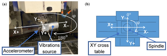
Figure 4.
Mid-sized milling machine with vibration source (a) schematic top view (b).
Direct dynamic compliance as a function of the angle at the first six eigenfrequencies (, , , , , and ) is plotted in Figure 5.
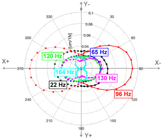
Figure 5.
Dynamic compliance polar diagram at selected frequencies.
The single-mass model for spindle representation with up to three degrees of freedom of general oscillation in 3D space is being examined (Figure 6). Modal transformation from physical coordinates to modal coordinates is chosen for model description. The frequency transfer function of the system is then expressed by the sum of the contributions of the three eigenmodes ( to ), which can be chosen for a specific case of a mechanical system to represent a significant part of the system dynamic properties. To create a model, it is necessary to know the weight of the spindle mass. Unknow stiffness values of the springs in the model are found by fitting the experimentally obtained frequency transfer functions.
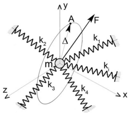
Figure 6.
Three degrees of freedom oscillation model.
- Displacement in the force direction
- Natural frequency
- Modal damping
- Eigenvectors
- Directional force cosine vector
Transfer function allows the model to have three eigenfrequencies with the respect of 3D space and two eigenfrequencies in the plane area for .
By substituting for in Equation (3), the surface of direct static compliance can be obtained. There are six points of contact touching the embraced non-rotary ellipsoid of compliance (see Figure 7) where the real force application points are when the 3D space force is applied in the whole spherical steradian range (this could be described as a certain form of Lamé’s stress ellipsoid used in the analysis of the tension tensors in the classical flexibility theory applied to homogenous materials).
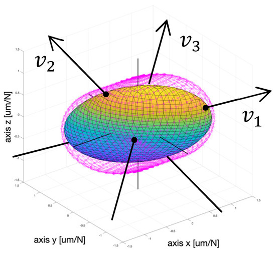
Figure 7.
Direct static compliance surface (magenta) with inscribed ellipsoid of compliance.
The direct dynamic compliance surface can be displayed separately for each eigenmode, see Figure 8 for the example of the first eigenmode of the system shown in Figure 7.
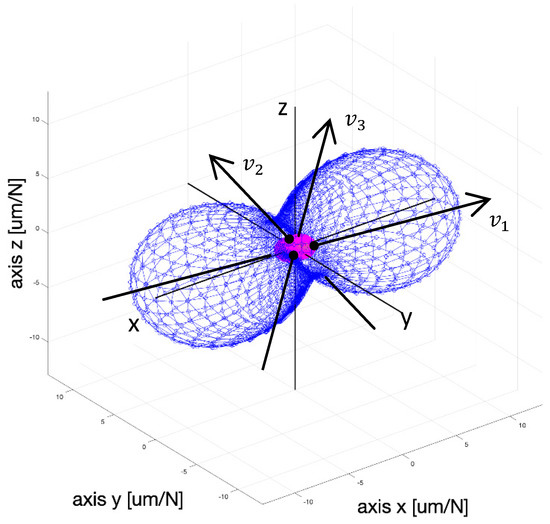
Figure 8.
Model of the direct dynamic (blue shape) and static compliance (magenta shape, as in Figure 7).
Previous experiments done on a lathe [4] have proven that the 2D plane oscillating system model is acceptable for simplification to oscillation only in the XY plane, perpendicular to the Z axis, which means for mathematical identification based on the Equation (3), only can be taken into account.
4. Structural Model of Feed Drive Axis
This chapter deals with approaches used to create linear axis models. The linear motion axis of a machine tool is approximated using one-mass or N-mass systems.
4.1. One-Mass Model of Linear Motor Feed Drive
A single-mass model can be used to represent the linear motor feed drive. A cascade control system with velocity PI and position P controller is shown in Figure 9. The direct transfer function in the system endpoint can be written as . represents the external force acting on the mass closest to the motor-first mass (can be easily replaced by the increased current input). stands for the transistor converter transfer function. Its transport delay can be replaced by the Padé approximation. Filters, which are not shown in the control system (usually low-pass and band-stop filters), may be included in the transfer function . The major feature of the position controller is that , meaning that the static compliance is equal to zero at .
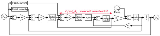
Figure 9.
Cascade regulation with linear motor block diagram (filters are not included).
4.2. N-Mass Model of Linear Motor Feed Drive
More complex mechanical structures can be described by a N-mass model, as illustrated in Figure 10. The motor input force is denoted as , excitation force used for feed drive diagnostics is denoted as , and the machining force acting at the mechanical system end point is denoted as .
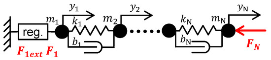
Figure 10.
N-mass system with regulation.
The mechanical model dynamic compliance matrix is a symmetric matrix derived from the mass, damping, and rigidity matrixes with a dimension . Mass matrix is diagonal, dumping matrix and stiffness matrix are band symmetric matrixes. All the sub–transfer functions of have the same denominator ( polynomial expression).
Assuming only and as acting forces, position and can be evaluated as:
The motor force acts on the first mass and the cutting force on the last mass. That means that the relevant model transfer functions are only corner expressions:
The motion axis block scheme is shown in Figure 11. The complete current control is labeled by symbol only. N-mass system dynamics is represented by the quadrupole, which is composed of the transfer functions in Equation (6).
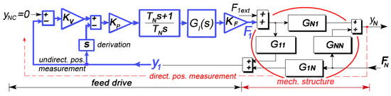
Figure 11.
Block diagram for system dynamic compliance evaluation.
The introduced block diagram can be algebraically described by following two equations:
4.3. General Dynamic Compliance Matrix of Mechanic Structure and Feed Drive Control
The coupled system of mechanics and feed drive control, described by the transfer function matrix GR (s), with inputs on the motor F1ext and on the N-mass FN and with corresponding outputs y1 and yN, is expressed by the diagram in Figure 12.
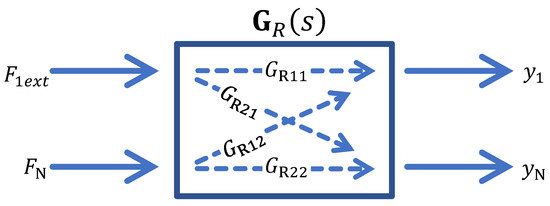
Figure 12.
N-mass system with regulation -quadrupole scheme.
Transfer function covers the controller dynamics (according to the blue highlighted part in Figure 11).
The general dynamic compliance matrix includes the complete cascade control, which is as symmetrical as the (introduced in Equation (4)) but has only dimension (two inputs and two outputs). Every sub-transfer function of matrix is expressed as an algebraic transcript of the block diagram shown in Figure 11.
The sub-transfer functions have the same common feature, which is the identical denominator of each sub-transfer function . Only the indirect position measurement is taken into account. For the case where the cutting force , the motor force and the system is excited by , given, e.g., by white noise. The first two expressions of matrix are:
where: , based on Figure 11, Equations (7)–(9).
where: .
For the other case, where the system is excited by the external force and the first mass is not affected by , the inner motor force is still generated though , the last two expressions of matrix are:
where: .
where: .
The symmetry of the matrix follows from the mechanical model dynamic compliance matrix symmetry where , thus .
The relevant transfer function in the self-excited or chatter identification theory is . Experimental identification of this particular transfer function requires a powerful vibration source. The easiest way of identifying the stability limits based on this transfer function is to obtain the necessary parameters through the transfer function , which can be easily experimentally identified with the following:
- can be obtained from the motor current commutation position sensors.
- motor force can be simulated by the additional current source.
transfer function reconstruction follows based on Equations (11)–(14). This methodology can be applied to any milling machine axis.
5. Feed Drive Coupled Model of the Machining Center
This chapter describes the application of the models shown above. The model of mechanics with feed drive control is demonstrated on the example of the vertical milling center shown in Figure 2.
5.1. Machine Tool Spindle
In general, the 3D space one-mass model of the spindle, which was described in chapter 0, is simplified to a model with two degrees of freedom for the purpose of modeling the dynamics of a vertical machine in the XY plane (see Figure 4). In Equation (3), therefore, it is considered for . Figure 13 shows the real part of direct frequency dynamic compliance depending on the direction of . The real part minimum is found approximately at for the 100° direction.
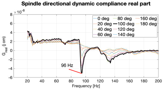
Figure 13.
Real part of spindle directional dynamic compliance.
5.2. Machine Tool XY Cross Table
A CAD model representing the mechanical structure is presented in Figure 14, and its dynamic scheme is in Figure 15.
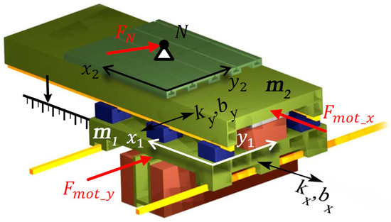
Figure 14.
XY cross table CAD model [19].
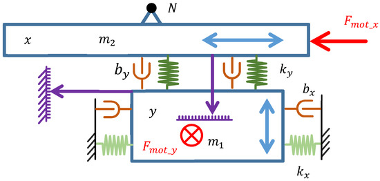
Figure 15.
Two-mass scheme of XY cross table.
5.2.1. X Axis
The one-mass model from the Figure 9 is applied with the following feed drive parameters , and obtained from the Sinumerik control system. It is not possible to describe this system as just one-mass with a direct position measurement due to the X axis coupling with the Y axis, therefore the model is improved by including the dynamic model of the traverse Y axis. Despite this coupling effect, the relevant bandwidth of the X axis is lower than the one that appears in the model caused by additional compliance in the Y axis (see the block diagram in the Figure 16. Real machine measurements and mathematical simulation are shown in the Figure 17). The parameters used for this simulation are based on the machine mechanical construction described in [19] and summarized in Table 1.
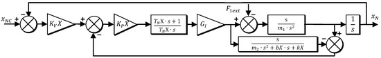
Figure 16.
Axis X linear motor one-mass system model.
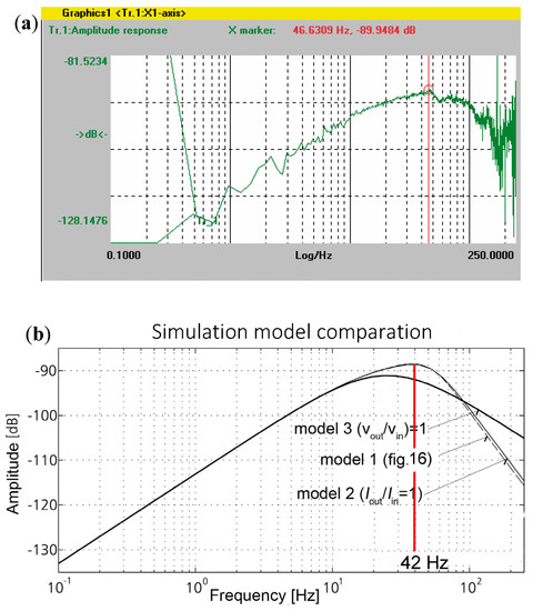
Figure 17.
Experimental measuring on the mid-sized vertical machine X axis (a), and mathematical simulation (b).

Table 1.
Axis X mechanical parameters.
Dynamic compliance determination was done within the control panel diagnostic environment, see Figure 17a. Identified simulation models (see Figure 17b) are divided based on the model complexity into:
- Model —represents the complete system shown in Figure 16 including inner ;
- Model —represents the system where the current transfer function is simplified: and is accepted for further modelling;
- Model —represents the system where the velocity transfer function is simplified: .
5.2.2. Y Axis
The two-mass model with the indirect position measurement is applied on the Y axis, shown in Figure 15 (the block diagram is identical to that shown in Figure 11). Transfer function is experimentally determined for the following parameters , , and obtained from the Sinumerik control system and the results can be seen in Figure 18. The experimental measurement is performed through the user interface of the Sinumerik machine control system using the disturbance frequency response type of measurement. A mathematical model is developed based on the motion axis mass values. The mathematical simulation is then obtained and compared with the measured values. The reconstructed transfer function (based on Equation (14)) is shown in Figure 19. Mechanical parameters are again obtained from [19] and summarized in Table 2.
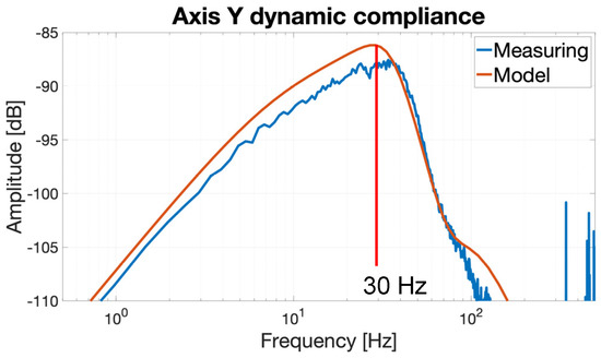
Figure 18.
Axis Y dynamic compliance .
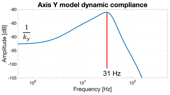
Figure 19.
Reconstructed axis Y model dynamic compliance
Table 2.
Axis Y mechanical parameters.
A significant advantage for the two-mass system is that the transfer function denominator can be solved directly from the mechanical structure dynamic compliance matrix as:
Adding up the direct dynamic compliances of the X, Y axes using the goniometric functions, the system of general dynamic compliances of the cross table is obtained for every applied force direction. Real parts of the dynamic compliance are then derived and shown in Figure 20. The degree-labeled directions are chosen so the directions in the cross table matches the direction in the middle measurement in Figure 5.
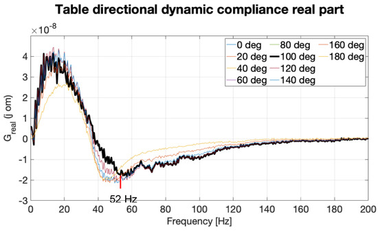
Figure 20.
Real part of the table directional dynamic compliance.
The resulting real parts of the dynamic compliance of the whole system including the spindle part and the XY cross table part in the measured directions are created by adding the spindle dynamic compliance from Figure 13 and cross table parts from Figure 20 together. The sum is in Figure 21; minimum values can be seen for each direction. For this direction, the two-mass system with mechanical parameters based on the spindle structure (detailed in Table 3) is taken into an account, see Figure 22 (including frequencies over is not relevant for the investigation of feed drive stability effect, which is why the model is not corresponding above this frequency).
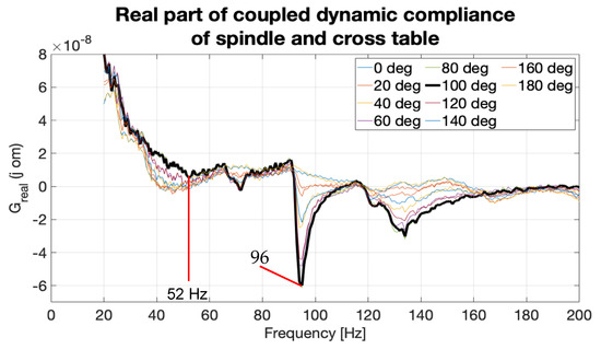
Figure 21.
Real part of coupled dynamic compliance of spindle and cross table.
Table 3.
Spindle model parameters.
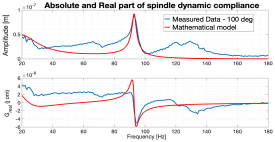
Figure 22.
Spindle and its model transfer function—100°.
Comparing the frequency domain with the minimum of the real part in Figure 20 (approximately ) and Figure 13 (approximately ), it can be seen that in the examined machine, there is a major compliance contribution by its spindle, see Figure 21. This result cannot be generalized and, in different machines the results can be preferable for the feed drive system, for example in machines with a sophisticated mechanical structure.
6. Impact of Feed Drive Control Parameters on Machining Stability Prediction
Identification for one direction of machining is processed. The angle of 100° was selected, see Figure 5, to demonstrate the influence of the feed drive parameters’ control on the overall stability in the machining process. Based on Formula (1) the critical depth of chip is determined by the minimum of the transfer function real part. Figure 23 shows a slight change in the lower frequencies (approximately ) based on the different constant tuning.
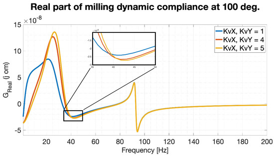
Figure 23.
Influence of constant on the real part of transfer function.
A construction of the resulting stability based on the feed drive parameters’ control of the SLD is shown in Figure 24. The shift is seen in the limiting depth of the cut based on the feed drive parameters’ control; in the presented case, the velocity regulation gain is applied. The critical depth of cut is given by the global real part minimum shown in Figure 23 for the frequency, approximately . The influence of feed drive parameters is seen in the area of .
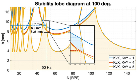
Figure 24.
Stability lobe diagram SLD diagram for various KV set-up
In the SLD in Figure 24, it is possible to focus on the shift in the depth of cut limits, for example, for the 50 revolutions per second (RPS) area. The comparison in cut difference is summarized in Table 4, where the 10.4% difference in the limit depth of cut as a local value is presented for the different feed drive parameter control.
Table 4.
Chip width limit for 50 RPS.
7. Conclusions
This paper describes modeling strategies of machine tool mechanics on an example of a mid-size vertical machining center. A one-mass model of the spindle with three degrees of freedom in 3D space is introduced. The model shows a significant directional dependence of the dynamic compliance for individual eigenmodes. An XY cross table model of the machine tool is represented by matrix of dimensions. Based on the fact that it is not always possible to experimentally measure the transfer function , the reconstruction from the experimentally measured transfer function was used.
The research focused on the impact of the XY cross table feed drive control parameters on the machining stability prediction using the developed model. In the direction with a deviation of only 10° from the X axis of the machine (in the text it is usually labeled as 100° direction), the most significant compliance of the spindle was found. In this direction, the resulting dynamic compliance between the spindle and the XY cross table was then coupled, and the influence of the proportional position loop gain on the prediction of machining stability limits was investigated. Compared to the initial setting of , a reduced setting of and an increased setting of was tested. The maximum increase in the stable chip depth occurs by approximately 11% when compared to and proportional position loop gain.
The study shows for the vertical machining center with linear motor feed drive, that a slight increase in the limit depth of cut can be achieved by changing the proportional position loop gain. However, this increase is limited to a narrow speed range of the stability gaps and therefore the practical use is very limited in a particular case but can be significant for machine tools with very low natural frequencies, where the dynamic compliance of the feed drive control coincides with the machine tool compliance.
Further research will be focused on verification of the dynamic properties of the spindle in the XY plane using experimental modal analysis and FEM computational models. Additionally, systematic research into the influence of velocity loop parameters and filters will be processed.
Author Contributions
Conceptualization, J.G. and P.S.; investigation, J.G. and P.S.; writing—original draft preparation, J.G.; writing—review and editing, M.S. and P.S. and J.G.; supervision, M.S. and P.S. All authors have read and agreed to the published version of the manuscript.
Funding
This research was funded by the Grant Agency of the Czech Technical University in Prague, grant number SGS19/165/OHK2/3T/12.
Conflicts of Interest
The authors declare no conflict of interest.
Nomenclature
| Controller dynamic transfer function | ||
| Damping coefficient | ||
| Critical depth of cut | ||
| Local limit depth of cut | ||
| Directional force cosine vector | ||
| Additional force transfer function | ||
| Mechanical model dynamic compliance matrix entries | ||
| Current transfer function | ||
| Mechanical part transfer function | ||
| Mechanical model dynamic compliance matrix | ||
| Cross table transfer function | ||
| General dynamic compliance matrix | ||
| General dynamic compliance matrix entries | ||
| Real part of G transfer function | ||
| Feed drive transfer function | ||
| Spindle transfer function | ||
| Velocity transfer function | ||
| Machine and drive transfer function | ||
| Current input signal | ||
| Current output signal | ||
| Stiffness | ||
| Cutting force coefficient | ||
| Force constant | ||
| Proportional velocity loop gain | ||
| Proportional current loop gain | ||
| Proportional position loop gain | ||
| Time delay | ||
| Velocity integration constant | ||
| Current integration constant | ||
| Displacement in the force direction | ||
| Eigenvectors | ||
| Velocity input signal | ||
| Velocity output signal | ||
| Linear scale | ||
| Requested chip thickness | ||
| Linear scale | ||
| Real cutting depth | ||
| Damping ratio | ||
| Modal damping | ||
| Natural frequencies | ||
| Chip width | ||
| Damping coefficients matrix | ||
| Acting forces vector | ||
| Acting forces | ||
| Finite Element Method | ||
| Stiffness matrix | ||
| Inductance | ||
| Mass matrix | ||
| Mass | ||
| Resistance | ||
| Rounds per second | ||
| Laplace operator | ||
| Stability lobe diagram | ||
| Axis direction | ||
| Actual position | ||
| Linear scale vector | ||
| [°] | Angle of measurement | |
| Frequency |
References
- Tlustý, J.; Poláček, M. The stability of machine tools against self-excited vibrations in machining, International Research in Production Engineering. Proc. ASME Int. 1963, 1, 465–474. [Google Scholar]
- Tobias, S.A.; Fishwick, W. Theory of regenerative machine tool chatter. Engineer 1958, 205, 199–203. [Google Scholar]
- Quintana, G.; Ciurana, J. Chatter in machining processes: A review. Int. J. Mach. Tools Manuf. 2011, 51, 363–376. [Google Scholar] [CrossRef]
- Grau, J.; Sulitka, M.; Souček, P. Influence of linear feed drive controller setting in CNC turning lathe on the stability of machining. J. Mach. Eng. 2019, 19, 18–31. [Google Scholar] [CrossRef]
- Altintas, Y.; Verl, A.; Brecher, C.; Uriarte, L.; Pritschow, G. Machine tool feed drives. CIRP Ann. 2011, 60, 779–796. [Google Scholar] [CrossRef]
- Albertelli, P.; Cau, N.; Bianchi, G.; Monno, M. The effects of dynamic interaction between machine tool subsystems on cutting process stability. Int. J. Adv. Manuf. Technol. 2012, 58, 923–932. [Google Scholar] [CrossRef]
- Lehotzky, D.; Turi, J.; Insperger, T. Stabilizability diagram for turning processes subjected to digital PD control. Int. J. Dyn. Control 2014, 2, 46–54. [Google Scholar] [CrossRef][Green Version]
- Beudaert, X.; Mancisidor, I.; Ruiz, L.M.; Barrios, A.; Erkorkmaz, K.; Munoa, J. Analysis of the feed drives control parameters on structural chatter vibrations. In Proceedings of the XIIIth International Conference on High Speed Machining, Metz, France, 4–5 October 2016. [Google Scholar]
- Franco, O.; Bedauert, X.; Erkorkmaz, K.; Barrios, A.; Munoa, J. Machining chatter stability limit improvement by means of feed drive control parameters. In Proceedings of the 8th International Conference on Virtual Machining Process Technology, Vancouver, BC, Canada, 24–25 April 2019. [Google Scholar]
- Franco, O.; Bedauert, X.; Erkorkmaz, K. Effect of Rack and Pinion Feed Drive Control Parameters on Machine Tool Dynamics. J. Manuf. Mater. Process. 2020, 4, 33. [Google Scholar] [CrossRef]
- Beudaert, X.; Franco, O.; Erkorkmaz, K.; Zatarain, M. Feed drive control tuning considering machine dynamics and chatter stability. CIRP Ann. 2020, 69, 1. [Google Scholar] [CrossRef]
- Nyquist, H. Regeneration Theory. Bell Syst. Tech. J. 1932, 11, 126–147. [Google Scholar] [CrossRef]
- Altintas, Y. Manufacturing automation: Metal cutting mechanics, machine tool vibrations, and CNC design. Appl. Mech. Rev. 2001, 54, B84. [Google Scholar] [CrossRef]
- Schmitz, T.L.; Smith, K.S. Machining Dynamics: Frequency Response to Improved Productivity; Springer: Berlin/Heidelberg, Germany, 2008. [Google Scholar]
- Altintas, Y.; Budak, E. Analytical Prediction of Stability Lobes in Milling. CIRP Ann. 1995, 44, 357–362. [Google Scholar] [CrossRef]
- Weck, M.; Brecher, C. Werkzeugmaschinen 5: Messtechnische Untersuchung und Beurteilung, dynamische Stabilität; Springer: Berlin/Heidelberg, Germany, 2006. [Google Scholar]
- Drobilek, J.; Polacek, M.; Bach, P.; Janota, M. Improved dynamic cutting force model with complex coefficients at orthogonal turning. Int. J. Adv. Manuf. Technol. 2019, 103, 2691–2705. [Google Scholar] [CrossRef]
- Souček, P.; Bubák, A. Vybrané Statě Z Kmitání V Pohonech Výrobních Strojů (The Chatter in Feed Drives of Production Machines: Summary); České vysoké učení technické: Praze, Czech Republic, 2008. [Google Scholar]
- Smolík, J.; Houša, J. Křížový Stůl S Lineárními Pohony Z Nekonvenčních Materiálů (Linear Feed Drive Cross Table Made of Unconventional Materials); Společnost pro obráběcí stroje: Praha, Czech Republic, 2000. [Google Scholar]
Publisher’s Note: MDPI stays neutral with regard to jurisdictional claims in published maps and institutional affiliations. |
© 2020 by the authors. Licensee MDPI, Basel, Switzerland. This article is an open access article distributed under the terms and conditions of the Creative Commons Attribution (CC BY) license (http://creativecommons.org/licenses/by/4.0/).