Learning-Based Prediction of Pose-Dependent Dynamics

Abstract

The constantly increasing demand for both, higher production output and more complex product geometries, which can only be achieved using five-axis milling processes, requires elaborated analysis approaches to optimize the regarded process. This is especially necessary when the used tool is susceptible to vibrations, which can deteriorate the quality of the machined workpiece surface. The prediction of tool vibrations based on the used NC path and process configuration can be achieved by, e.g., applying geometric physically-based process simulation systems prior to the machining process. However, recent research showed that the dynamic behavior of the system, consisting of the machine tool, the spindle, and the milling tool, can change significantly when using different inclination angles to realize certain machined workpiece shapes. Intermediate dynamic properties have to be interpolated based on measurements due to the impracticality of measuring the frequency response functions for each position and inclination angle that are used along the NC path. This paper presents a learning-based approach to predict the frequency response function for a given pose of the tool center point.

1. Introduction

Chatter vibrations are common challenges in milling processes, leading to an insufficient workpiece quality and reduced lifetime of the machine tool and cutting tools [1,2], especially if long and slender milling tools are necessary to machine the desired workpiece geometry [3,4,5,6]. Several approaches can be used to optimize the dynamic behavior of milling operations. The process stability can be evaluated analytically based on measured or simulated frequency response functions (FRFs) [7,8,9]. Furthermore, simulation approaches offer the possibility to reduce run-in periods of identifying suitable process parameter values and, thus, accelerate and simplify the process design and optimization, even for high process run-times [2,10,11]. For an optimization of milling processes with varying engagement conditions and complex desired workpiece shapes, geometric physically-based process simulations can be used [10]. In this context, the dynamic behavior of the compliant system, consisting of the combination of the machine tool, spindle, and cutting tool, can be modeled by a set of uncoupled, damped harmonic oscillators to represent the FRF of the system measured at the tool center point (TCP) [12]. For each oscillator of the set, the modal mass $m_{\mathrm{m}}$, the natural frequency $f_{\mathrm{m}}$ and the damping constant ${\gamma }_{\mathrm{m}}$ have to be identified. Subsequently, the process forces, exciting the compliance system and estimated by, e.g., applying an empirical force model, which has to be calibrated based on the used combination of tool geometry and workpiece material, can be used within the dynamic model. Thus, the deflections of the milling tool can be calculated and the process stability can be assessed. Additionally, stability lobe diagrams (SLD) can be calculated for different combinations of the process parameter values using suitable stability criteria. However, especially when machining free-formed surfaces of large workpieces, the pose-dependent load of the spindle bearings and axis drives influences the modal properties of the system significantly [11,13,14,15], resulting in different frequency response behaviors for each pose defined by the NC path.

Different methodologies have been investigated to model this influence. Kono et al. [16] investigated the influence of the rotation angle of a five-axis machine tool with swiveling table on the dynamic compliance and oscillations during a milling process by modal analysis. The maximum difference between the compliance amplitudes was about 40% when varying the B-axis angle. Multiple analytical approaches can be found in literature. In this regard, Budak et al. [17] presented analytical models for the cutting geometry, process forces and process stability for 5-axis milling operations. Shamoto and Akazawa [18] analytically calculated SLDs based on FRF measurements for a ball-end milling process with respect to different inclination angles. A reasonable agreement between measured and calculated stabilities could be achieved. When considering the modeling of pose-dependent dynamics, Du et al. [19,20] modeled the dynamic behavior of a bi-rotary milling head using multi-rigid-body dynamic models considering the varying stiffness of the flexible joints affected by gravity and cutting forces. Furthermore, Chao and Altintas [21] optimized the tool path for machining a free-formed surface by analytically analyzing the engagement conditions using FRFs which were measured in different poses. Regarding oscillations of thin-walled workpieces, Siebrecht et al. [22] used a barycentric interpolation approach for estimating the dynamic compliance of the workpiece at different positions on the surface.

In recent years, the use of machine learning (ML) methods in research activities regarding production engineering has increased drastically [23,24,25]. They offer the capability to deliver predictions of process characteristics for previously unseen process features and conditions with a reasonable accuracy. Thus, ML-based models were successfully trained in order to predict process forces [26,27,28,29], the surface roughness of the machined workpiece [30,31,32] and tool vibrations [33,34]. When considering SLDs, Friedrich et al. [35] realized an ML-based framework that was able to iteratively adapt an SLD based on continuous measurements during process conduction. In addition, Denkena et al. [36] learned SLDs based on measured data and investigated the suitability of different methods. There are few publications dealing with the prediction of pose-dependent dynamics based on ML methods. In this context, a transfer learning approach was presented by Chen et al. [37], whereby a multilayer perceptron (MLP), which was trained using a high amount of data originating from impact hammer tests, was adapted to be valid for different cutting tools using only few additional data. However, FRFs with only one single dominant mode were considered and no SLDs were derived for the regarded configurations.

In this paper, an investigation of the prediction of FRFs and the subsequent fitting of corresponding oscillator-based compliance models is presented in order to enable the interpolation between poses for which FRFs were acquired by impact hammer tests. Using an evolutionary-based algorithm, an automated parameterization of compliance models using an initial set of parameter values, estimated by a single manual fitting procedure, could be derived to reduce the amount of manual fitting procedures for given FRFs. Furthermore, SLDs were generated using the resulting compliance models and a geometric physically-based simulation approach. These SLDs are compared to the experimentally determined stability limits using acoustic emission signals for different inclination angles, visualizing the usefulness of the approach for an optimization of five-axis milling operations. The SLDs are also compared to SLDs that were acquired using compliance models predicted by ML models directly, skipping the investigation of FRFs at the interpolation poses. In addition, the advantages and disadvantages of both approaches are discussed in detail. Different methods of ML were used for the learning objectives to evaluate their suitability. The paper is structured, as follows. In Section 2, the technological investigations, which were conducted to acquire FRFs for different poses using two machine tools and the acoustic emission signals for different inclination angles, are described in detail. The geometric physically-based simulation system, which was applied to estimate SLDs, is introduced in Section 3. The identification of the modal parameter values of the oscillator-based compliance models to represent FRFs while using an evolutionary algorithm is explained in Section 4. Section 5 presents the learning objectives and the used base-line methods, which were applied to perform the interpolation of FRFs and compliance models. The results of the learning tasks for two different five-axis machine tools are presented, evaluated and discussed in Section 6. In addition, Section 6 also comprises the results of comparing SLDs for predicted FRFs as well as predicted compliance models to stabilities, retrieved by an evaluation of acoustic signals of corresponding milling processes. The paper concludes with a summary of the conducted investigations (see Section 7).

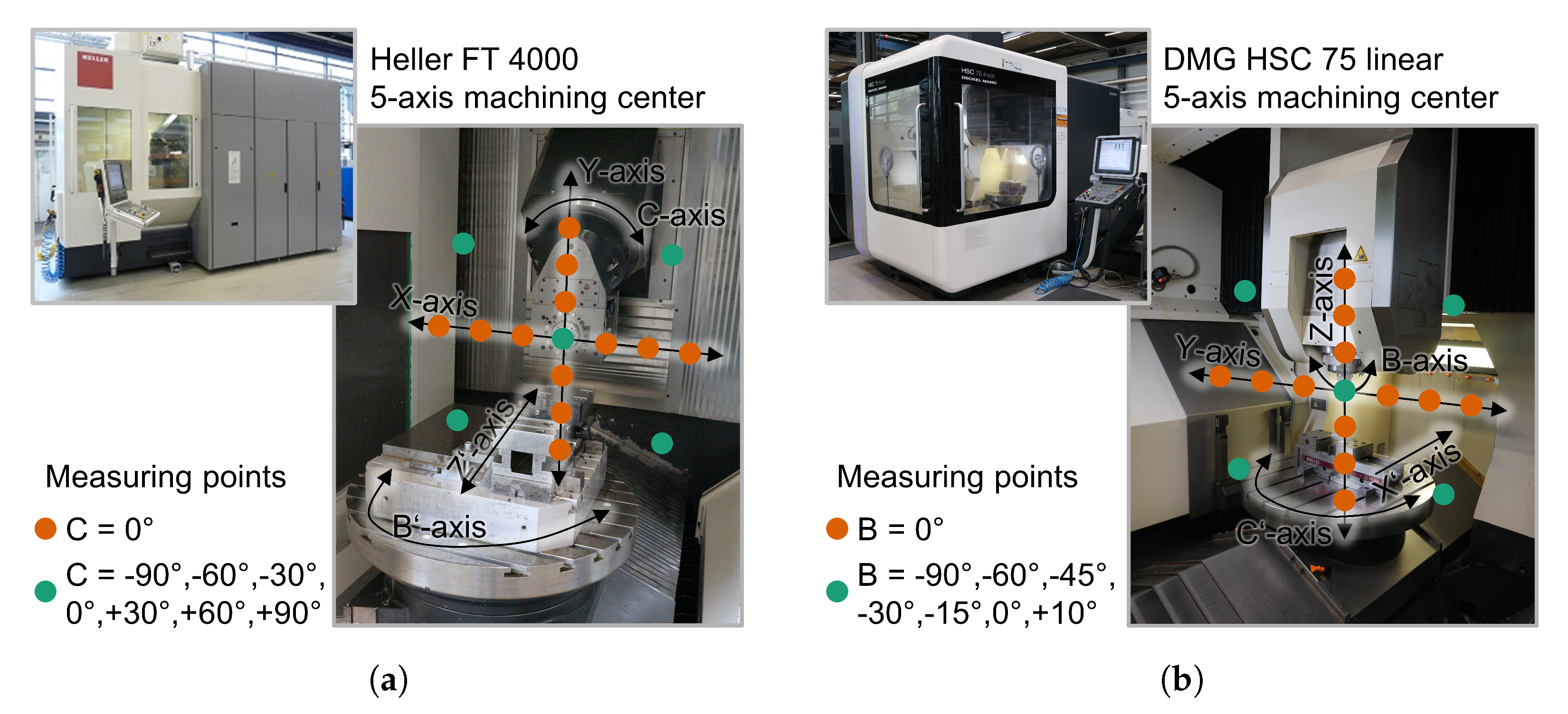
2. Technological Investigation

For the acquisition of a sufficient training set and, therewith, validation of the presented method, frequency response measurements were performed through impact hammer tests on two machine tools in different poses. On a five-axis machining center with swivel head kinematic Heller FT 4000, denoted as $M_1$ in the following, the positions of the axes influencing the pose of the tool, X, Y, and C, were varied. Furthermore, on a five-axis machining center with fork head kinematic DMG HSC 75 linear, denoted as $M_2$, the Y-, Z-, and B-axis positions were varied. For both of the machining centers, the axis positions were selected on the basis of an extended centrally composed experimental design with star points, in order to be able to investigate higher order influences as well as possible cross-correlations (cf. Figure 1). A total number of $P_1=46$ and $P_2=49$ poses were investigated using $M_1$ and $M_2$, respectively.

All of the axis positions were defined in the machine coordinate system allowing the axes to be moved individually over the whole working area of the machine tools (cf.

Table 1. Range of the investigated axis positions for both machine tools.

Machine Tool	M1		M2
Range of investigated axis positions	X	$-400$ mm to $+400$ mm	Y	0 mm to $+600$ mm
	Y	$+100$$\mathrm{m}$$\mathrm{m}$ to $+900$ $\mathrm{m}$$\mathrm{m}$	Z	$-400$$\mathrm{m}$$\mathrm{m}$ to 0 $\mathrm{m}$$\mathrm{m}$
	C	$-90$${}^{\circ }$ to $+90$ ${}^{\circ }$	B	$-90$${}^{\circ }$ to $+10$${}^{\circ }$

).

The FRF measurements were conducted using a Fraisa X7400 spherical end mill with a diameter of $d=10 \mathrm{mm}$ and a free length of $l_{\mathrm{l}}=30.4 \mathrm{mm}$. Hereto, an impact hammer Kistler 8206 and an acceleration sensor 352C23 by PCB Piezotronics, mounted at the tool tip, were used. Fast Fourier transformations were performed up to $f_{\max ,}1=6400 \mathrm{Hz}$ and $f_{\max ,}2=3200 \mathrm{Hz}$ for $M_1$ and $M_2$, respectively. The finite length of the impulse response function measurements led to a frequency resolution of $∆f_1=0.25 \mathrm{Hz}$ and $∆f_2=0.5 \mathrm{Hz}$ for $M_1$ and $M_2$, respectively.

Slot milling experiments were conducted using the aforementioned milling tool, the machine tool $M_2$, and an increasing depth of cut $a_{\mathrm{p}}$, using a starting value of $a_{\mathrm{p},\mathrm{start}}$ and a depth of cut of $a_{\mathrm{p},\mathrm{end}}$ at the end of each slot, in order to validate the calculated SLDs. A high speed steel ASP 2012 hardened to approx. 58 HRC was machined. Different inclination angles and spindle speeds were investigated. There are different publications in literature, which investigated the detection of chatter vibrations applying wavelet analysis using various signals, e.g., cutting forces [38] or tool accelerations [39,40,41]. In this contribution, discrete acoustic emission signals were recorded and analyzed utilizing the continuous wavelet transform [42]

$$\begin{array}{c}\hfill W(a,b)=\sum _{i=1}^N{\xi }^{\left(i\right)}{\left(\frac{{\delta }_t}{a}\right)}^{\frac{1}{2}}{\mathrm{\Psi }}^{*}\left[\frac{(i-b){\delta }_t}{a}\right]\end{array}$$

(1)

for each experiment. In this context, ${\xi }^{\left(i\right)}$ is the i-th sample of the original acoustic emission signal, N is the total number of samples of the signal, ${\mathrm{\Psi }}^{*}$ is the complex conjugate of a mother wavelet $\mathrm{\Psi }$, ${\delta }_t$ is the time difference between two samples of the signal, and a and b are the scaling and translation variables, respectively. Each scaled and translated mother wavelet corresponds to an investigated frequency at a time instant. By calculating the convolution between the original signal and the scaled and translated mother wavelet, the correlation between the signal and a frequency can be estimated for each time instant. For the mother wavelet, the complex Morlet wavelet [43]

$$\begin{array}{c}\hfill \mathrm{\Psi }\left(\eta \right)={\pi }^{-\frac{1}{4}}{e}^{i{\omega }_0\eta }{e}^{-\frac{{\eta }^2}{2}}\end{array}$$

(2)

was used. The stability limit $a_{\mathrm{p},\mathrm{crit}}$ of each experiment was estimated as

$$\begin{array}{c}{a}_{\mathrm{p},\mathrm{crit}}=a_{\mathrm{p},\mathrm{start}}+\frac{i_{\mathrm{crit}}·\left(a_{\mathrm{p},\mathrm{end}}-a_{\mathrm{p},\mathrm{start}}\right)}{N},\end{array}$$

(3)

$$\begin{array}{c}{i}_{\mathrm{crit}}=i\in \left\{\mathbb{N}|\bigcap _{a}T(W^{\left(i\right)}\left(a\right),N_T)>\overline{W\left(a\right)}+\tau ·W_{\mathrm{s}}\left(a\right),\forall i\in \left\{1,\cdots ,N\right\},\forall a\in S\right\},\end{array}$$

(4)

whereby $W\left(a\right)$ is the wavelet transform of the signal, $\tau$ is a user-defined threshold value and S is the set of investigated scales, which correspond to a set of natural frequencies of the FRF of the regarded pose. For the Morlet wavelet, the relationship between a scale a and the Fourier period $\lambda$ can be described as

$$\begin{array}{c}\lambda =\frac{4\pi a}{{\omega }_0+\sqrt{2+{\omega }_0^2}},\end{array}$$

(5)

whereby ${\omega }_0$ is the non-dimensional central frequency of the mother wavelet. Because natural frequencies measured for a non-rotating spindle may differ from natural frequencies of a rotating system, the function $T(W^{\left(i\right)}\left(a\right),N_T)$ calculates a weighted average of the wavelet intensities, incorporating $N_T$ neighboring frequencies of the natural frequency, which corresponds to the scaling a. For the weighting, the Blackman window function [44]

$$\begin{array}{c}w\left(j\right)={\alpha }_0-{\alpha }_{1}cos\left(\frac{2\pi j}{N_T}\right)+{\alpha }_{2}cos\left(\frac{4\pi j}{N_T}\right)\end{array}$$

(6)

with

$$\begin{array}{c}\hfill {\alpha }_0=0.42,{\alpha }_1=0.5,{\alpha }_2=0.08\end{array}$$

(7)

was used, whereby $W^{\left(i\right)}\left(a\right)$ was weighted with $w(N_T/2)$. Equation (4) represents different values for the translation variable b with the index i, assuming that there is a set $\left\{W^{\left(i\right)}\left(a\right)\forall i\in \left\{1,\cdots ,N\right\}\right\}$, whereby each $W^{\left(i\right)}\left(a\right)$ corresponds to a sample ${\xi }^{\left(i\right)}$ of the original signal and b is estimated according to the temporal location of ${\xi }^{\left(i\right)}$ within the time series. Thus, the stability limit is estimatednby identifying a critical index $i_{\mathrm{crit}}$, which is defined as the index, where each of the weighted averages of wavelet intensities of a frequency and its neighboring frequencies of a set of investigated natural frequencies exceeds $\overline{W\left(a\right)}+\tau ·W_{\mathrm{s}}\left(a\right)$, whereby

$$\begin{array}{cc}\hfill \overline{W\left(a\right)}& =\frac{1}{N}\sum _{i=1}^N{W}^{\left(i\right)}\left(a\right),\end{array}$$

(8)

$$\begin{array}{cc}\hfill W_{\mathrm{s}}\left(a\right)& =\sqrt{\frac{{\sum }_{i=1}^N{(W^{\left(i\right)}\left(a\right)-\overline{W\left(a\right)})}^2}{N-1}}\end{array}$$

(9)

are the mean and the standard deviation of a wavelet transform $W\left(a\right)$, respectively. Figure 2 visualizes the identification of the stability limit using a spindle speed of n = 3025 min⁻¹ and an inclination angle of $B=-45{}^{\circ }$.

Acoustic emission signals often are highly influenced by noise. As a result, a high amount of frequencies correlate with the corresponding scaled and translated wavelet transforms. The natural frequencies 1415 $\mathrm{Hz}$, 1500 $\mathrm{Hz}$ and 1580 $\mathrm{Hz}$ of the three dominant peaks of the FRF in X- and Y-direction were considered when analyzing the wavelet transform, since they were expected to have the most influence on the stability behavior of the process. Using the aforementioned approach, a stability limit of $a_{\mathrm{p},\mathrm{crit}}=0.5\mathrm{mm}$ was identified, since all og the wavelet transforms, which corresponded to the three natural frequencies, exceeded the defined threshold at the corresponding point in time. The stability limits, which are calculated using the presented method, have to be interpreted with caution. The resulting limits are highly dependent on the signal-to-noise ratio of the acoustic emission signal and the choice of $\tau$. As a result, the transferability to processes that differ from the considered configuration is limited.

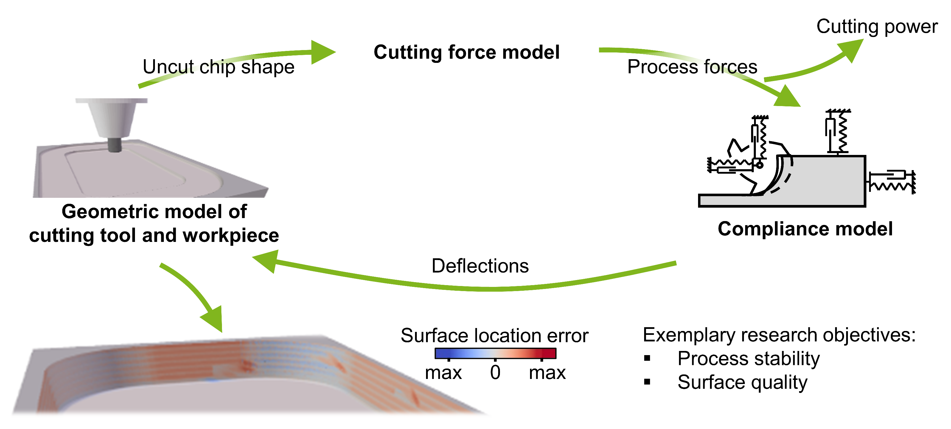
3. Geometric Physically-Based Simulation of Milling Processes

In general, geometric physically-based process simulations combine geometric representations of the milling tool and workpiece with physically-based models in a time-discrete manner in order to offer predictions for various process characteristics [2]. These characteristics usually comprise macroscopic effects such as process forces, process dynamics and the resulting surface errors of the machined workpiece surface, which can be modeled by incorporating and combining different models [10,45]. Apart from milling processes, grinding [46] and honing [47] processes or process chains [48] can also be analyzed.

In this contribution, a simulation system was used, which is described in detail by Wiederkehr and Siebrecht [2]. The constructive solid geometry (CSG)-technique [49] was used to analyze the uncut chip shape for each simulation time step by intersecting the models of tool and workpiece (cf. Figure 3) [50].

The resulting process forces were calculated using an empirical force model [51,52], which can be described as

$$\begin{array}{cc}\hfill F_i& =k_i·b·h_0·{\left(\frac{h}{h_0}\right)}^{(1-c_i)},\hfill \\ \hfill i& \in \{c,n,t\},\hfill \end{array}$$

(10)

for the cutting, normal and tangential direction, respectively, whereby $h_0=1\mathrm{mm}$, h is the uncut chip thickness, b is the width of the cutting slices, which represent the spacial discretization of the cutting edges of the geometric model of the cutting tool and $k_c$, $k_n$, $k_t$, $c_c$, $c_n$, and $c_t$ are the model parameters. Machining experiments were conducted using the process parameter values defined in

Table 2. Process parameter values.

Tool Diameter	Workpiece Material	Spindle Speed	Depth of Cut	Radial Immersion	Inclination Angle
10 mm	ASP 2012 (58 HRC)	$5445{\min }^{-1}$	$0.1$ mm	100%	$-20$${}^{\circ }$, $-30$${}^{\circ }$, $-45$${}^{\circ }$

in order to parametrize the model parameter values. The force model parameter values were identified using a gradient-based optimization algorithm [53]. Because the uncut chip thickness remains constant for different inclination angles and its nonlinear influence on the process forces is insignificant for the subject under investigation a linear cutting force model could be assumed. Thus, the exponent in Equation (10) was set to 1, i.e., $c_i=0.0$.

The identified parameter values of the force model for different inclination angles are summarized in

Table 3. Parameter values of cutting force model.

Inclination Angle (${}^{\circ }$)	${\mathit{k}}_{\mathbf{c}}$ (N mm ${}^{-2}$)	${\mathit{k}}_{\mathbf{t}}$ (N mm ${}^{-2}$)	${\mathit{k}}_{\mathbf{n}}$ (N mm ${}^{-2}$)	${\mathit{m}}_{\mathbf{c}}$	${\mathit{m}}_{\mathbf{n}}$	${\mathit{m}}_{\mathbf{t}}$
$-20$	8745	$\mathrm{12,546}$	337	$0.0$	$0.0$	$0.0$
$-30$	7333	$\mathrm{10,711}$	436	$0.0$	$0.0$	$0.0$
$-45$	6651	$\mathrm{10,246}$	612	$0.0$	$0.0$	$0.0$

.

A compliance model based on uncoupled, damped harmonic oscillators for representing FRFs was used for simulating the resulting deflections of the tool and evaluating the process stabilities [12,54]. As discussed by Surmann and Enk [54], a set of Poincaré points were used to calculate the diameter of the Poincaré section, which was used as stability criterion. Each Poincaré point was defined two-dimensionally as the magnitudes of the deflections in X- and Y-direction at the beginning of each tooth engagement. The diameter of the Poincaré section was then calculated as the diagonal length of the smallest rectangle, which could be defined around the set of considered Poincaré points. The smaller the diameter, the higher the assumed process stability. For each combination of depth of cut and spindle speed in the regarded range of the parameter values, simulations were conducted and the resulting stabilities were evaluated in order to generate SLDs for a given inclination angle.

4. Fitting of Parameter Values of Compliance Models

In order to represent FRFs, either measured or predicted compliance models were used in X- and Y-direction of the tool coordinate system according to the method proposed by Surmann et al. [12]. These consisted of a set of uncoupled damped harmonic oscillators separately for the X- and Y-direction. Each oscillator was parameterized by identifying values for the modal mass $m_{\mathrm{m}}$, the natural frequency $f_{\mathrm{m}}$, and the damping constant ${\gamma }_{\mathrm{m}}$. The parameterized models were used to calculate the complex response function

$$\begin{array}{c}\hfill \begin{array}{cc}\hfill G{\left(\omega j\right)}_d& =\sum _{q=1}^Q\left(cos\left({\varphi }_d^{\left(q\right)}\left(\omega \right)\right)·A_d^{\left(q\right)}\left(\omega \right)+sin\left({\varphi }_d^{\left(q\right)}\left(\omega \right)\right)·A_d^{\left(q\right)}\left(\omega \right)·j\right),d\in \{x,y\}\hfill \\ \hfill A\left(\omega \right)& =\frac{\frac{1}{m_{\mathrm{m}}}}{\sqrt{{\left({\omega }_{\mathrm{m}}^2-{\omega }^2\right)}^2+4·{\gamma }_{\mathrm{m}}^2{\omega }_{\mathrm{m}}^2}},\hfill \\ \hfill \varphi \left(\omega \right)& ={tan}^{-1}\left(\frac{2{\gamma }_{\mathrm{m}}\omega }{{\omega }_{\mathrm{m}}^2-{\omega }^2}\right),\hfill \\ \hfill {\omega }_{\mathrm{m}}& =2\pi f_{\mathrm{m}}\hfill \end{array}\end{array}$$

(11)

according to the amplitude and phase resulting from each oscillator q for each investigated angular frequency $\omega$. The results were then compared to the measured FRFs to calculate the optimization loss. Therefore, the resulting problem is an optimization problem of parameter values and can be solved by a genetic algorithm [55]. Genetic algorithms are inspired by the concept of natural evolution and use selection, mutation, and crossover methods to evolve a population of solution candidates to retrieve an optimized result [56,57]. The candidates are called individuals and consist of a set of parameter values which is a possible solution for the problem, where the quality is defined by a fitness function [56]. For the oscillator fitting, one individual is a set of $3·Q$ parameters, where Q is the number of oscillators. To initialize the individuals of the starting population of the automated fitting procedure using the genetic algorithm, oscillators for the X- and Y-direction were generated manually for one FRF of each machine. Subsequently, the fitness values were calculated according to the inverse of

$$\begin{array}{c}\hfill \mathcal{L}=\sum _i{\left({\widetilde{A_t}}^{\left(i\right)}-{\widetilde{A_p}}^{\left(i\right)}\right)}^2+\sum _i{\left({\widetilde{{\varphi }_t}}^{\left(i\right)}-{\widetilde{{\varphi }_p}}^{\left(i\right)}\right)}^2,\end{array}$$

(12)

which represents the sum of the squared error between the normalized values of the calculated amplitude $\widetilde{A_p}$ and phase values $\widetilde{{\varphi }_p}$ and the normalized measured data $\widetilde{A_t}$ and $\widetilde{{\varphi }_t}$ for the investigated frequency range. The normalization was performed according to the minimum and maximum values of the amplitudes and phases to transform the values, which were used by the fitness function, to the range 0–1. Subsequently, the individuals of one population were sorted according to the corresponding fitness values in ascending order. Operations of selection, mutation, and crossover were used to estimate the next generation of individuals. The mutation function added a random value between $-2$ $\mathrm{Hz}$ and 2 $\mathrm{Hz}$ to $f_{\mathrm{m}}$ of the considered oscillator and used a deviation of up to 2% to modify $m_{\mathrm{m}}$ and ${\gamma }_{\mathrm{m}}$. Applying the crossover method, the oscillators of two selected individuals, from 30% of the actual generation that achieved the best fitness values, were mixed. This procedure was repeated until a total amount of 1000 iterations were conducted or if the best fitness value did not improve for 20 iterations.

An analysis of the measured FRFs resulted in the assumption that there were frequencies above the considered frequency measurement range, which were relevant to achieving a reasonable fitting result at the upper frequency limit. Therefore, an additional oscillator with fixed parameter values was added, whose natural frequency was above the measurement range. Figure 4 shows an exemplary comparison of the measured and calculated FRFs, where the calculation was based on an evolutionary parameter optimization of oscillator-based compliance models.

The calculated FRFs in Figure 4a are based on compliance models whose natural frequencies lie inside the considered frequency measurement range. Unfortunately, using this strategy, the fitting results were not suitable to accurately represent the measured frequency response behavior. There clearly was a phase angle shift at the end of the frequency range, indicating the necessity of another oscillator whose natural frequency is outside of the frequency range. Because no reference measurements were present to consider this oscillator within the parameter optimization, an oscillator with the fixed parameter values $f_{\mathrm{m}}=3807.51\mathrm{Hz}$, ${\gamma }_{\mathrm{m}}=2236.61\frac{1}{\mathrm{s}}$ and $m_{\mathrm{m}}=0.04\mathrm{k}\mathrm{g}$ for X-direction and $f_{\mathrm{m}}=3582.16\mathrm{Hz}$, ${\gamma }_{\mathrm{m}}=1527.42\frac{1}{\mathrm{s}}$ and $m_{\mathrm{m}}=0.09\mathrm{k}\mathrm{g}$ for Y-direction was included to the oscillator set of each compliance model. Using this approach, a suitable fit could be achieved for each FRF of each considered pose. Nevertheless, there was an uncertainty regarding the accuracy of the representation of the frequency response behavior above the frequency measurement range, which was neglected in the following investigations.

5. ML Methods for Predicting Pose-Dependent Dynamics of Milling Processes

Two learning objectives were considered in this paper. For both objectives, let $\mathcal{X}$ be a set of $J\times N$ features, sampled from an unknown distribution $\mathcal{D}$, and $\mathcal{Y}$ be a set of $K\times N$ targets, labeled by some target function. The first objective comprised the prediction of FRFs. For this, the measured FRFs of all P considered measuring poses were discretized into data points by the frequency resolution $∆f$, so that M is the number of investigated frequencies for each pose. Each of the $N=P·M$ data points contained a number of K targets, comprising the compliance amplitude and phase shift for the X- and Y-direction of the machine coordinate system. Let J be the number of features, consisting of the frequency and positions of the three axes that define the pose. For the second learning objective, which represented the prediction of modal parameter values for given poses, let J consist of the three pose-dependent features and $N=P$. For the targets, let $K=3·(Q_x+Q_y)$, whereby $Q_x$ and $Q_y$ are the number of oscillators in X- and Y-direction, respectively. Using this approach, the learning task tried to also represent the relationship between different interdependent oscillators of each compliance model, even across the two different oscillation directions. For both learning objectives, the goal was to find a learner $h:\mathcal{X}\to \mathcal{Y}$ with respect to the distribution $\mathcal{D}$. Because $\mathcal{D}$ is unknown to the learner, the true prediction error cannot be calculated. To mitigate this problem, the empirical risk ${\mathcal{L}}_D\left(h\right)$ was employed. In practice, it is desirable to find a learner, such that

$$\begin{array}{c}\hfill {\mathcal{L}}_D\left(h\right)=\underset{x\sim \mathcal{D}}{\mathbb{E}}{(h\left(x\right)-y)}^2\end{array}$$

(13)

is minimized. This paradigm is often denoted as empirical risk minimization.

Several learning-based methods can be used for approaching regression objectives. The simplest models can be trained while using linear regression [58,59], whereby the relationship between the features and the targets are assumed to be

$$\begin{array}{c}\hfill \mathcal{Y}=\beta ·\mathcal{X}+ϵ.\end{array}$$

(14)

The parameters $\beta$ are the coefficient of the model and the error term $ϵ$ represents all of the deviations between forecasts and $\mathcal{Y}$ which cannot be represented by the model. One of the most popular approaches for fitting a linear model to a set of training data is the least-squares method. In this context, the approach tries to identify the model coefficients $\beta$, which minimize the sum of squared residuals

$$\begin{array}{c}\hfill \begin{array}{cc}\hfill \mathrm{RSS}\left(\beta \right)& =\sum _{i=1}^N{(y_i-x_i\beta )}^2\hfill \\ \hfill & ={(\mathcal{Y}-\mathcal{X}\beta )}^T(\mathcal{Y}-\mathcal{X}\beta ).\hfill \end{array}\end{array}$$

(15)

Setting the first derivative of Equation (15) to zero, the unique solution is given by

$$\begin{array}{c}\hfill \widehat{\beta }={\left({\mathcal{X}}^T\mathcal{X}\right)}^{-1}{\mathcal{X}}^T\mathcal{Y},\end{array}$$

(16)

if ${\mathcal{X}}^T\mathcal{X}$ is invertible. The simplicity of linear regression, which offers highly interpretable model instances, entails several issues, e.g., either delivering a poor prediction accuracy or the trained model suffers from severe overfitting. This bias-variance dilemma [60] can be addressed through several regularization techniques. In this contribution, the elastic net [61] was used as a regularization approach, which combines the ${\ell }_1$ and ${\ell }_2$ norms of the model coefficients, such that

$$\begin{array}{c}\hfill \begin{array}{cc}\hfill \widehat{\beta }& =\underset{\beta }{argmin}\sum _{i=1}^{N}l(y_i,x_i\beta )+{\mu }_2{\left|\beta \right|}^2+{\mu }_1{\left|\beta \right|}_1,\hfill \\ \hfill {\left|\beta \right|}^2& =\sum _{p=1}^{J·K}{\beta }_p^2,\hfill \\ \hfill {\left|\beta \right|}_1& =\sum _{p=1}^{J·K}\left|{\beta }_p\right|,\hfill \end{array}\end{array}$$

(17)

where ${\lambda }_1$ and ${\lambda }_2$ are regularization parameters. Using this approach, the elastic net tries to overcome issues, which arise when using either ridge [62] or least absolute shrinkage and selection operator (LASSO) [63] regression. While penalizing the size of $\beta$ through the ${\ell }_2$ norm in the context of ridge regression leads to lower variance, coefficients of highly correlated variables tend to be shrunk together. Using LASSO, a sparse solution is encouraged by incorporating the ${\ell }_1$ norm, which aims to make the model more interpretable. However, although no shrinkage of coefficients is done, LASSO simply picks one of the group of coefficients of highly correlated variables. No systematics of the selection can be derived, depending on the context. Elastic net attempts to stabilize this selection procedure by shrinking and selecting sparsely simultaneously, realizing a compromise between ridge and LASSO.

Another popular approach to reduce overfitting effects is the use of ensemble techniques [64,65], whereby a set of weak learners $h_b\left(x\right)$ with high bias are utilized to generate a strong combined learner. Usually the weak learners are tree-based models mostly trained using the classification and regression trees (CART) algorithm [66], but the choice of the used model is arbitrary. Several strategies emerged for the combination of the weak learners. In bootstrap aggregation (bagging) [67], each weak learner is trained using a different subset of the training set. This subset is sampled with replacement, which means that an observation can be in multiple subsets. For regression objectives, the final prediction of the combined learner can be summarized as

$$\begin{array}{c}\hfill \widehat{y}=\frac{1}{B}\sum _{b=1}^B{h}_b\left(x\right).\end{array}$$

(18)

In this paper, random forests (RF) [68] were used, which can be categorized to bagging techniques. While training a RF, opposing to the algorithms of classical decision tree learning, the split is performed using a randomly sampled set of features, also known as feature subsampling. Using boosting [69], a sequential approach is performed for the combination of the weak learners. At each iteration, the model

$$\begin{array}{c}\hfill H_b\left(x\right)=H_{b-1}\left(x\right)+{\rho }_b·h_b\left(x\right)\end{array}$$

(19)

tries to learn from mistakes of the previous iteration, whereby the step length ${\rho }_b$ is usually estimated by line search. As a popular example of boosting algorithms, XGBoost [70] was additionally used in this contribution. XGBoost is a specific parallelized implementation of the gradient boosting (GB) technique [71], whereby each weak learner is fitted to the residuals of the previous learner by formulating the objective as a gradient descent optimization procedure. The regularized objective

$$\begin{array}{c}\hfill \begin{array}{cc}\hfill \mathcal{L}\left(H\right)& =\sum _{i=1}^{N}l\left({\widehat{y}}_i,y_i\right)+\sum _{b=1}^M\mathrm{\Omega }\left(h_b\right),\hfill \\ \hfill \mathrm{\Omega }\left(h\right)& =\kappa T+\frac{1}{2}\mu {\left|\beta \right|}^2,\hfill \end{array}\end{array}$$

(20)

penalizes both the number of leaves T and the size of the weights $\beta$ of the leaves of each tree $h_b$, whereby l is a loss function, representing the difference between ${\widehat{y}}_i$ and $y_i$. This addition aims to reduce overfitting in a similar manner than using the ridge regularization in the context of linear regression. Furthermore, feature subsampling, originating from RF, is used when performing the tree split to further reduce overfitting and speed up the training procedure. An approximation algorithm is conducted to improve the runtime efficiency when utilizing tree boosting using the XGBoost algorithm, instead of performing an exact greedy search, which iterates over all possible splits over all features. This algorithm tries to find the best split that identifies a set of candidate splits according to the proposed distributed weighted quantile sketch algorithm.

6. Results

The following section presents the results for the two considered learning tasks, i.e., the prediction of FRFs and the prediction of parameter values of compliance models, in order to reduce the measurement effort and to enable the possibility to retrieve information about the pose-dependent dynamic behavior of milling operations for poses that were not investigated technologically. For both learning tasks, different strategies for defining the training and test sets were investigated. As described in Section 2, FRFs were measured for a total amount of 46 and 49 poses while using $M_1$ and $M_2$, respectively. In addition to randomly choosing four poses for testing, another strategy for choosing poses for the test set was to use all poses that use a certain inclination angle, whereby three different test angles were considered in total for each machine and each investigated base-line method. The remaining poses were used for training. The test angles $C=-30{}^{\circ }$, $C=-60{}^{\circ }$ and $C=120{}^{\circ }$ were used for $M_1$ and $B=-20{}^{\circ }$, $B=-30{}^{\circ }$ and $B=-45{}^{\circ }$ were used for $M_2$. This resulted in a total amount of five test poses for each test angle of each machine tool, except for a test angle of $B=45{}^{\circ }$ for $M_2$, where four test poses were examined. In order to measure the deviation between measured and predicted data, the root-mean-square error (RMSE)

$$\begin{array}{c}\hfill {\mathrm{RMSE}}_k=\sqrt{\frac{{\sum }_{i=1}^N{({\widehat{y}}_k^{\left(i\right)}-y_k^{\left(i\right)})}^2}{N}}\end{array}$$

(21)

for each target $y_k$ was used. The results that were achieved by applying the ML base-line methods were also compared to a naïve linear interpolation approach for both learning objectives. In this contest, the pose-dependent features were organized in a k–d tree [72]. For each test pose, a previously specified number of nearest neighboring poses were identified in the k-d tree. Subsequently, each calculated target value for the test pose resulted from a weighted average of the target values from the neighboring training poses. The weights were chosen according to the distance between the test pose and the respective training poses. A parameter that significantly influenced the interpolation accuracy was the number of incorporated neighboring poses. Each possible number of neighbors from a range of 2–20 was examined and the best performing configuration was used to generate the reported results.

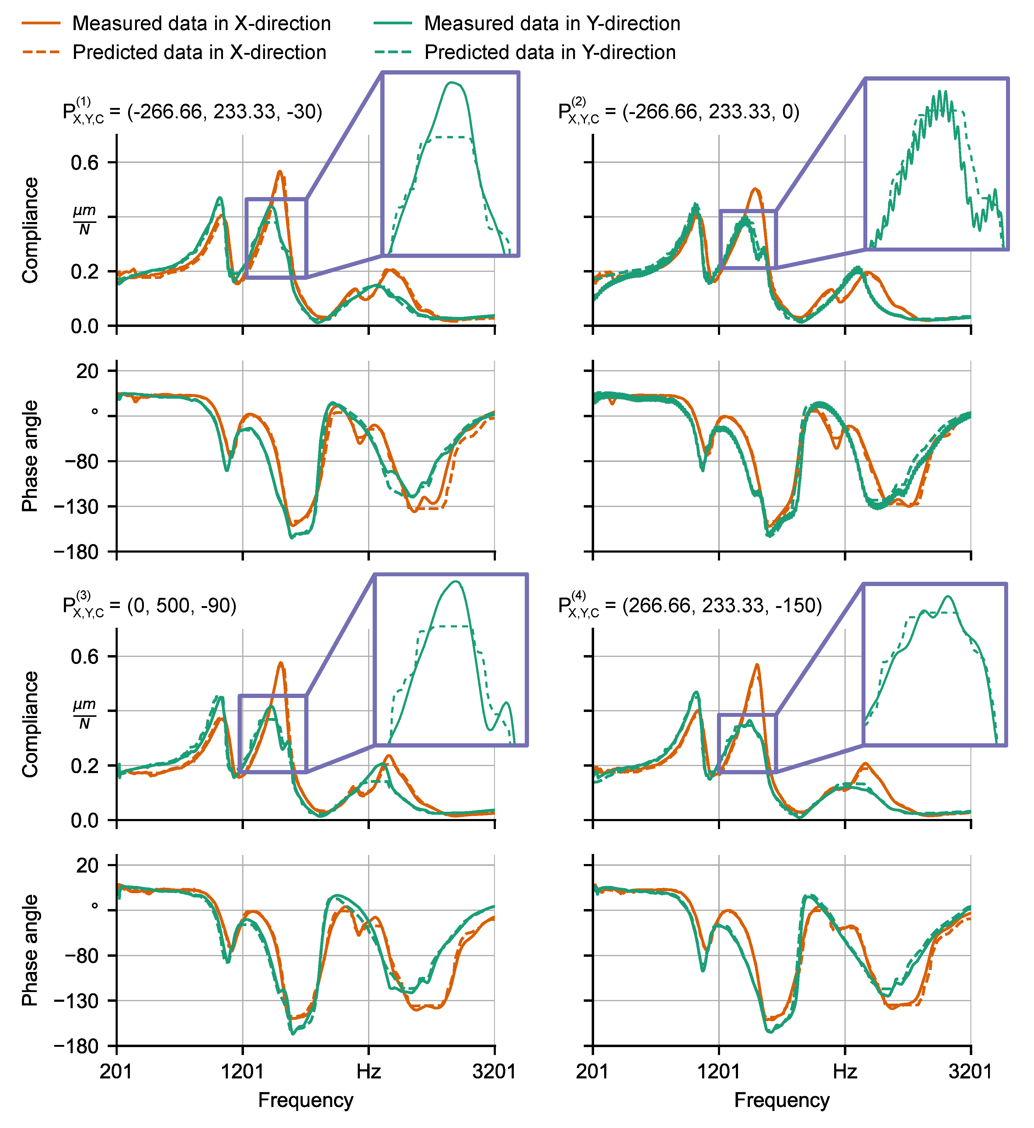
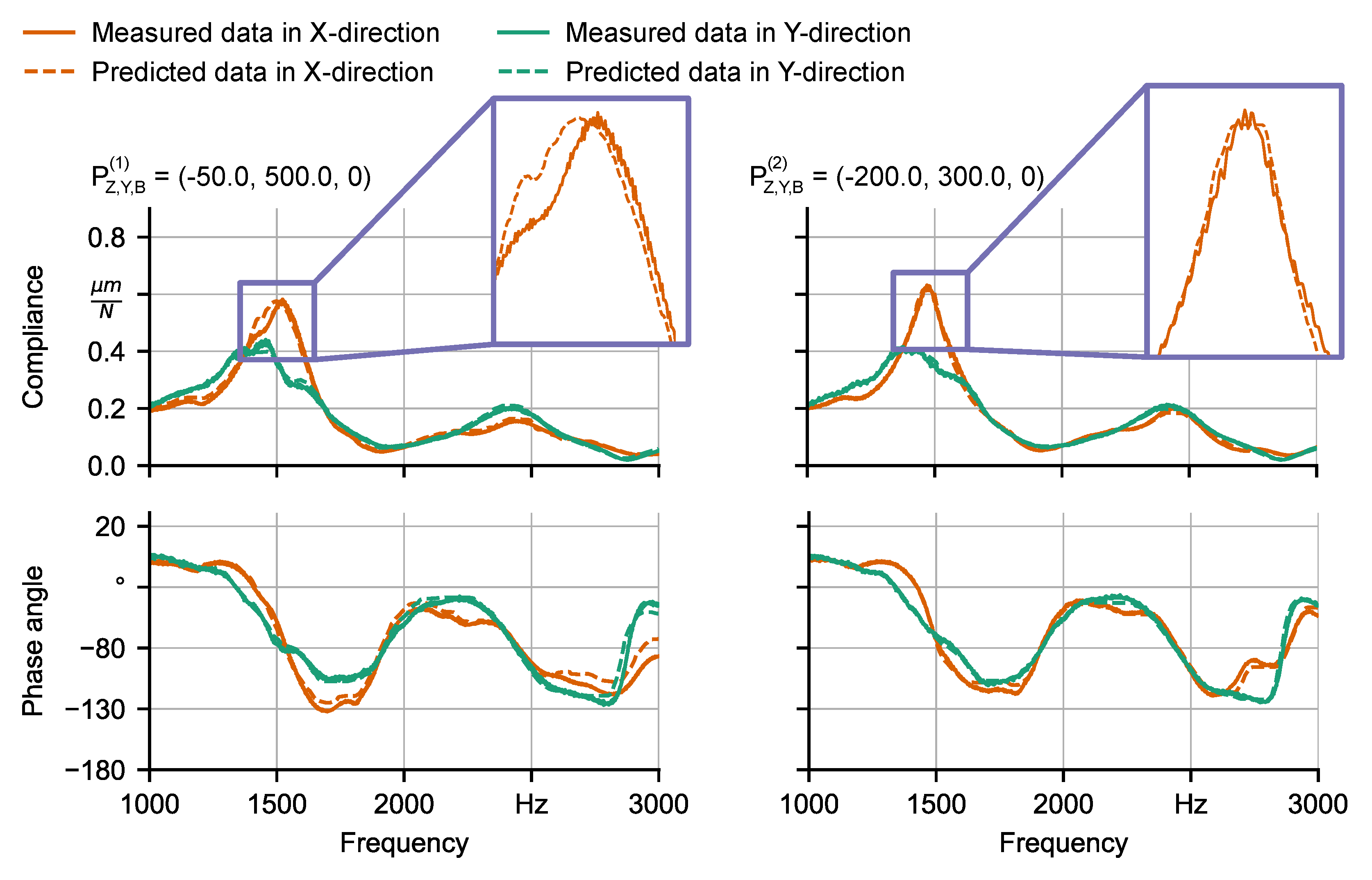
6.1. Learning of FRFs

In the context of this learning objective, $J=4$, since the three pose properties and the frequency were considered to be features. Furthermore, $K=4$, comprising the values for the amplitude and phase for the X- and Y-direction. Figure 5 shows a comparison between FRFs that were measured using the machine tool $M_1$ and predicted FRFs using RF for four different test poses that were not included in the training set.

The considered poses were $P_{\mathrm{X},\mathrm{Y},\mathrm{C}}^{\left(1\right)}=(-266.66,233.33,-30)$, $P_{\mathrm{X},\mathrm{Y},\mathrm{C}}^{\left(2\right)}=(-266.66,233.33,0)$, $P_{\mathrm{X},\mathrm{Y},\mathrm{C}}^{\left(3\right)}=(0,500,-90)$ and $P_{\mathrm{X},\mathrm{Y},\mathrm{C}}^{\left(4\right)}=(266.66,233.33,-150)$ and contained the corresponding values for X, Y and C of the pose, respectively. The phases could be predicted with a high accuracy in both, X- amd Y-direction, for all considered test poses, except for a visible deviation for $P_{\mathrm{X},\mathrm{Y},\mathrm{C}}^{\left(1\right)}$ between 2200–2500 $\mathrm{Hz}$. This could be explained by the measured behavior of the phase being quite unique among all measured phases in this frequency range, resulting in the model failing to achieve an accurate prediction. The amplitudes in X-direction were predicted with a nearly non-visible deviation from the measured curves for all test poses. There are two peaks visible in measured FRFs in Y-direction in a frequency range of 1200–1700 Hz, which are very distinct for $P_{\mathrm{X},\mathrm{Y},\mathrm{C}}^{\left(2\right)}$ and $P_{\mathrm{X},\mathrm{Y},\mathrm{C}}^{\left(3\right)}$. For $P_{\mathrm{X},\mathrm{Y},\mathrm{C}}^{\left(1\right)}$, the second peak can hardly be detected and for $P_{\mathrm{X},\mathrm{Y},\mathrm{C}}^{\left(4\right)}$, the second peak is not present. This behavior could be represented by the model to a certain extent. The fusion of the two peaks for $P_{\mathrm{X},\mathrm{Y},\mathrm{C}}^{\left(4\right)}$ could successfully be predicted. In addition, the model also predicted a visible second peak for the remaining test poses, but the differences in the distinction between the two peaks across the poses could not be achieved. This effect was very minor in the investigated data and has to be analyzed in more detail in future research activities. In order to represent such behavior, more observations in which the fusion of peaks is present and that can be considered for the training procedure would be necessary.

Figure 6 shows a comparison between measured FRFs using the machine tool $M_2$ and predicted FRFs using XGBoost, which was the best performing method in this case, for two different test poses.

There was a high accordance between the measured and predicted phase angles in X- and Y-direction. The difference between measured and predicted amplitudes in X- and Y-direction was also very low. Although the width and hight of the amplitudes in X-direction could successfully be predicted, there was a deviation of the shape of the curves in the range between 1300–1700 $\mathrm{Hz}$. This deviation also corresponds to a fusion of peaks, since there are two peaks visible for $P_{\mathrm{Z},\mathrm{Y},\mathrm{B}}^{\left(1\right)}$, which could not be accurately predicted, and only one peak for $P_{\mathrm{Z},\mathrm{Y},\mathrm{B}}^{\left(1\right)}$, whereby the difference between measurement and prediction is low. This emphasizes the already concluded statement about more observations being necessary to predict these effects.

Table 4. Comparison between the root-mean-square error (RMSE) of predicted amplitudes and phases in X- and Y-direction of the machine coordinate system for two machine tools using different methods.

Method	Machine Tool	Test Angle (${}^{\circ }$)	RMSE (N/$\mathsf{\mu }$m) Amplitude X-direction	RMSE (N/$\mathsf{\mu }$m) Amplitude Y-Direction	RMSE (${}^{\circ }$) Phase X-Direction	RMSE (${}^{\circ }$) Phase Y-Direction
Naïve linear interpolation	$M_1$	$-30$	0.02 ± 0.01	0.01 ± 0.01	6.15 ± 4.39	7.57 ± 6.08
		$-60$	0.02 ± 0.01	0.01 ± 0.01	7.95 ± 5.75	5.75 ± 4.44
		$-120$	0.02 ± 0.02	0.02 ± 0.01	7.25 ± 4.98	7.57 ± 5.39
		Random	0.02 ± 0.01	0.02 ± 0.02	5.47 ± 3.94	8.91 ± 6.69
	$M_2$	$-20$	0.01 ± 0.01	0.01 ± 0.01	4.30 ± 3.05	6.73 ± 5.24
		$-30$	0.02 ± 0.01	0.01 ± 0.01	5.61 ± 3.75	4.85 ± 3.55
		$-45$	0.02 ± 0.02	0.01 ± 0.01	7.34 ± 5.17	3.90 ± 2.75
		Random	0.02 ± 0.02	0.01 ± 0.01	7.16 ± 4.84	5.64 ± 4.29
Elastic net	$M_1$	$-30$	0.11 ± 0.07	0.09 ± 0.06	38.28 ± 23.04	42.37 ± 24.80
		$-60$	0.11 ± 0.07	0.09 ± 0.06	38.66 ± 22.34	43.62 ± 25.41
		$-120$	0.10 ± 0.07	0.09 ± 0.06	38.83 ± 21.71	42.70 ± 25.08
		Random	0.11 ± 0.08	0.10 ± 0.06	38.55 ± 23.25	42.05 ± 25.21
	$M_2$	$-20$	0.11 ± 0.08	0.08 ± 0.05	31.22 ± 17.09	30.50 ± 13.37
		$-30$	0.11 ± 0.08	0.08 ± 0.05	31.55 ± 17.46	30.24 ± 13.46
		$-45$	0.12 ± 0.08	0.08 ± 0.04	31.91 ± 17.39	30.17 ± 12.97
		Random	0.14 ± 0.10	0.10 ± 0.06	31.48 ± 16.93	29.52 ± 13.05
RF	$M_1$	$-30$	0.01 ± 0.01	0.01 ± 0.01	5.07 ± 3.67	6.01 ± 4.99
		$-60$	0.02 ± 0.01	0.01 ± 0.01	5.46 ± 3.94	5.07 ± 3.87
		$-120$	0.02 ± 0.01	0.01 ± 0.01	5.80 ± 3.85	6.34 ± 4.51
		Random	0.01 ± 0.01	0.01 ± 0.01	4.53 ± 3.39	5.71 ± 4.42
	$M_2$	$-20$	0.01 ± 0.01	0.01 ± 0.01	3.28 ± 2.29	4.67 ± 3.46
		$-30$	0.01 ± 0.01	0.01 ± 0.01	3.83 ± 2.58	5.57 ± 4.14
		$-45$	0.01 ± 0.01	0.01 ± 0.01	2.58 ± 1.72	3.08 ± 2.15
		Random	0.02 ± 0.01	0.01 ± 0.01	5.64 ± 3.67	4.32 ± 3.09
XGBoost	$M_1$	$-30$	0.01 ± 0.01	0.01 ± 0.01	4.22 ± 2.86	6.31 ± 5.05
		$-60$	0.02 ± 0.01	0.01 ± 0.01	5.23 ± 3.72	4.96 ± 3.91
		$-120$	0.02 ± 0.01	0.01 ± 0.01	5.35 ± 3.58	5.34 ± 3.73
		Random	0.01 ± 0.01	0.01 ± 0.01	4.54 ± 3.37	6.03 ± 4.62
	$M_2$	$-20$	0.01 ± 0.01	0.01 ± 0.01	2.85 ± 2.06	4.17 ± 3.09
		$-30$	0.01 ± 0.01	0.01 ± 0.01	3.77 ± 2.58	4.60 ± 3.28
		$-45$	0.01 ± 0.01	0.01 ± 0.01	2.05 ± 1.29	2.89 ± 1.92
		Random	0.02 ± 0.02	0.01 ± 0.01	5.48 ± 3.60	4.41 ± 3.18

shows the results of learning FRFs for the two investigated machine tools while using different methods and different inclination angles for testing, which were not used during training.

In general, using the elastic net regression was not successful for both machine tools, since the RMSE is about 10 times higher than using other methods. Surprisingly, the naïve linear interpolation performed significantly better than the elastic net regression, which is also based on a linear model, although these results were still, on average, approximately 25% worse than the results of the ensemble methods. This emphasizes the possibility to model the relationship between the axis poses and frequency-based machine tool dynamics linearly with reasonable accuracy. The low prediction accuracy of the elastic net could be a result of an unsuccessful regularization leading to overfitting. When comparing the results of RF with the ones achieved by using XGBoost, the bagging technique performed slightly better on average, but, overall, both ensemble methods delivered a reasonably low RMSE. Predicting FRFs for fixed inclination angles delivered slightly better results than randomly chosen angles. This might be counter-intuitive at first sight. An explanation for this could be the randomly chosen test set comprising scenarios, whose relationship between poses, frequencies, amplitudes, and phases were not represented by the training set.

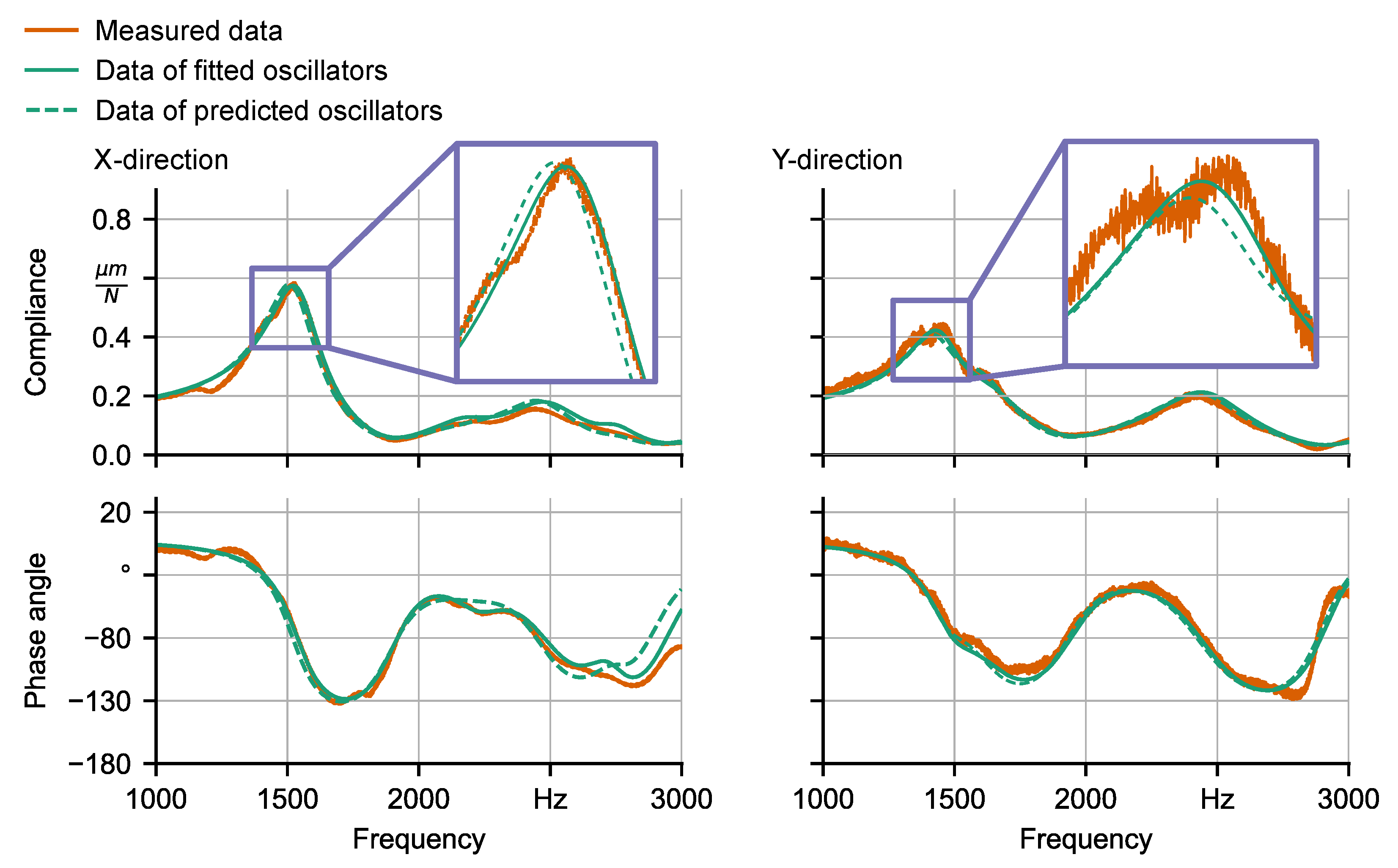
6.2. Learning of Oscillator Parameter Values

In contrast to learning FRF, the learning of parameter values of oscillator-based compliance models, whose results are presented in the following, tried to represent the relationship between information about specific poses and compliance model instances, which would result from parameter optimization procedures. A major advantage of this approach is that it enables the possibility to retrieve information about pose-dependent dynamic behaviors through an evaluation of learned models, which, in contrast to conducting a fitting procedure of oscillator parameter values, can be performed in real-time. In the context of this learning task, $J=3$, only comprising the pose-related values. No frequency information has to be provided, since this learning task skipped the prediction of frequency response behaviors and aimed to represent the properties of compliance models directly, given a certain pose. Furthermore, as described in Section 5, $K=3·(Q_x+Q_y)$, representing the parameter values of a set of oscillators. A number of $Q_x=5$ and $Q_y=4$ were chosen to model the measured FRFs by the evolutionary-based fitting procedure, which was necessary to generate the training and test sets, in the X- and Y-direction, respectively.

Figure 7 shows an exemplary comparison between a measured FRF, an FRF calculated using a compliance model that results from the fitting procedure, which is described in Section 4, and an FRF resulting from predicted parameter values of a compliance model according to the second learning objective for the pose $P_{\mathrm{Z},\mathrm{Y},\mathrm{B}}=(-50.0,500.0,0.0)$ and the machine tool $M_2$.

Generally, a high accordance was observed. Examining the zoomed-in areas of the FRFs, it can be seen that the shape of the measured FRF could only be coarsely represented by the evolutionary-based fitting procedure. Because the fitted oscillator parameter values served as target values for the learning objective, the FRF, which was calculated based on predicted oscillator parameter values, could not reproduce the measured behavior in higher detail than the FRF, which resulted from the fitting procedure. Nevertheless, there were only small deviations between the fitted and predicted data, which was also concluded based on the results of

Table 5. Comparison between the RMSE of the predicted modal parameter values for two machine tools using different methods.

Method	Machine Tool	Test Angle (${}^{\circ }$)	RMSE (Hz) Mean Frequency	RMSE (1/s) Mean Damping Constant	RMSE (kg) Mean Mass
Naïve linear interpolation	$M_1$	$-30$	31.71 ± 7.54	108.22 ± 15.15	0.09 ± 0.04
		$-60$	27.91 ± 7.16	126.09 ± 21.63	0.16 ± 0.10
		$-120$	25.00 ± 6.15	79.63 ± 18.88	0.06 ± 0.01
		Random	22.80 9.13	124.43 36.97	0.09 0.01
	$M_2$	$-20$	9.95 ± 4.20	252.86 ± 58.68	0.92 ± 0.19
		$-30$	12.06 ± 3.67	329.58 ± 5.40	1.35 ± 0.24
		$-45$	12.96 ± 3.26	399.25 ± 64.87	1.28 ± 0.29
		Random	23.17 ± 20.93	376.27 ± 456.82	0.90 ± 1.15
Elastic net	$M_1$	$-30$	24.35 ± 6.63	117.18 ± 45.63	0.07 ± 0.03
		$-60$	22.78 ± 6.15	86.06 ± 38.50	0.05 ± 0.02
		$-120$	23.49 ± 5.96	93.34 ± 28.51	0.04 ± 0.02
		Random	27.83 ± 8.44	89.37 ± 18.93	0.07 ± 0.04
	$M_2$	$-20$	9.04 ± 3.32	200.36 ± 50.46	0.65 ± 0.13
		$-30$	9.94 ± 1.48	158.15 ± 42.03	0.51 ± 0.26
		$-45$	8.98 ± 3.41	146.53 ± 32.06	0.35 ± 0.14
		Random	22.65 ± 19.65	292.88 ± 363.70	0.77 ± 0.67
RF	$M_1$	$-30$	23.90 ± 6.46	106.38 ± 45.23	0.06 ± 0.02
		$-60$	23.30 ± 6.95	80.51 ± 33.53	0.05 ± 0.02
		$-120$	23.40 ± 5.99	90.22 ± 30.91	0.04 ± 0.02
		Random	27.54 ± 9.05	90.25 ± 18.57	0.06 ± 0.04
	$M_2$	$-20$	7.56 ± 3.47	68.75 ± 23.22	0.23 ± 0.11
		$-30$	10.30 ± 2.54	79.31 ± 24.98	0.27 ± 0.14
		$-45$	9.28 ± 4.46	86.67 ± 38.51	0.23 ± 0.14
		Random	21.05 ± 20.21	387.27 ± 344.32	1.04 ± 0.78
XGBoost	$M_1$	$-30$	24.28 ± 8.00	94.68 ± 40.28	0.05 ± 0.02
		$-60$	23.77 ± 4.80	107.50 ± 46.74	0.04 ± 0.02
		$-120$	24.05 ± 5.47	98.15 ± 29.58	0.05 ± 0.02
		Random	27.27 ± 10.44	83.01 ± 19.11	0.07 ± 0.04
	$M_2$	$-20$	7.70 ± 2.84	71.17 ± 32.38	0.25 ± 0.18
		$-30$	11.45 ± 3.45	85.40 ± 34.32	0.33 ± 0.14
		$-45$	8.74 ± 3.69	87.39 ± 52.48	0.43 ± 0.17
		Random	21.49 ± 21.05	435.98 ± 447.16	1.22 ± 1.01

. Therefore, the learning of oscillator parameter values directly from given poses could be interpreted as successful.

Table 5 shows the results of learning oscillator parameter values directly for given poses for different inclination angles for the test set using different methods.

It can be seen that even the elastic net delivered suitably low RMSE scores, especially for predicting the natural frequency of the oscillator models. The naïve linear interpolation provided the lowest performance and achieved on average approximately 31% worse results than the results of the ensemble methods. For the damping constant and the modal mass, a superior performance of the ensemble models could be observed, indicating a more non-linear relationship between the pose and the damping constant and the modal mass than between the pose and the natural frequency. Similar to the first learning objective, randomly chosen test scenarios were significantly harder to predict than using a fixed inclination angle for the test set.

A trade-off has to be considered summarizing the results of evaluating the two regarded learning objectives. Applying the first objective of learning FRFs, the measured behavior could mostly be represented in detail while deviations between measured and predicted data were observed when a fusion of amplitude peaks of the frequency response was present. A higher prediction accuracy should be expected when acquiring a higher number of observations for the training set, which more prominently represent the behavior of fused peaks. If an application of a geometric physically-based simulation system is pursued to, e.g., simulate SLDs or visualize simulated location errors on the workpiece surface based on an evaluation of oscillator-based compliance models, a fitting of the parameter values of the compliance model has to be performed following each prediction of an FRF. Because this has to be conducted for each pose of the used NC path, the run-time of simulation executions would increase significantly, negating one of the major advantages of geometric simulation approaches. Nevertheless, this approach could be very useful for applications in methods that perform stability calculations in the frequency-domain. These are, e.g., the analytical stability calculation method by Altintaş and Budak [7] or the impulse dynamic subspace method proposed by Dombovari et al. [73] used to calculate time-domain-based process simulations directly based on frequency response functions. However, predicting parameter values of oscillators directly without considering the underlying FRF given a pose of the NC path by realizing the second learning objective, no deterioration of simulation run-times is expected. This is due to the capability to evaluate ML models in real-time, so that no fitting procedure is required. By using this approach, a more coarse representation of the frequency response behavior has to be tolerated that results from the automatic evolutionary-based fitting procedure, which was used to generate the training set for the learning task. The fitting procedure has to be performed in both cases, but at various stages of the realization sequence, i.e., following the ML-based prediction of each FRF for the first learning objective or following the measurement of each FRF to generate the training set in the context of the second learning task. Thus, the loss of information is inevitable, relativizing the disadvantages of the second learning objective to a certain extent. However, information of the frequency response behavior for a given pose, where no FRF information was measured, can only be acquired by using the first learning objective. Finally, even a naïve linear interpolation of target values for both learning objectives delivered acceptable results, although it performed worse overall than the ML-based methods. If a time-consuming training procedure of model instances is to be avoided at all costs, this is still a valid approach for generating usable results.

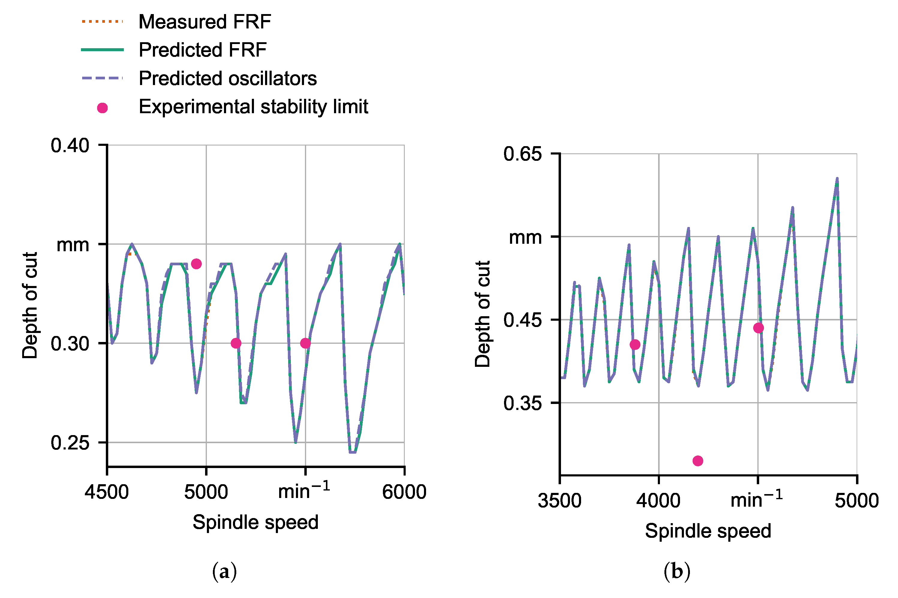
6.3. Comparison between SLDs

Figure 8 shows a comparison between SLDs that were calculated by using a geometric physically-based simulation system (see Section 3), fitted compliance models (see Section 4), resulting from either using measured (see Section 2) or predicted FRFs and predicted compliance models (see Section 5).

In addition, the SLDs are compared to experimentally identified stability limits according to the approach that is described in Section 2. In this context, $\tau \in [2,2.5]$ and the choice was made based on expert domain knowledge. The differences between the SLDs can hardly be identified visually, indicating a high applicability of both learning approaches for identifying stable process parameter values as compared to using measured FRFs. However, high deviations between simulated and experimentally determined stability limits can be observed for certain values for the spindle speed. Nevertheless, these deviations could result from inaccurate simulation results and are unlikely a consequence of poor prediction accuracies from the approaches presented in this contribution, since there were no visible deviations between the individual SLDs. The inaccuracy of simulation results can be rooted in several reasons, e.g., neglecting process damping and tool wear or calibrating the compliance models using FRFs, which were measured for a non-rotating tool while the experimentally determined stability limits were a result of analyzing acoustic emission signals of milled slots, obviously using a rotating tool. Moreover, compliance models were only used in the X- and Y-direction. These models were excited using directed force vectors, enabling the calculation of tool deflections based on a weighted interpolation of compliances in X- and Y-direction if the direction of excitation is not exactly aligned with either of these directions. However, the cross FRFs, which represent the relationships between perpendicular directions of excitation and response, were not taken into account. In addition, the solutions of the gradient-based identification of the coefficients of the force model are not unique [74], leading to a limited transferability from calibration experiments to experiments with different engagement situations between the tool and workpiece.

7. Conclusions

In this paper, an investigation of predicting process dynamics using ML methods for different machine poses is presented. In this context, measurements of FRFs for different poses while using two different machine tools were conducted by utilizing impact hammer tests. An evolutionary-based optimization procedure was used to identify modal parameter values for compliance models that consisted of a set of uncoupled, damped harmonic oscillators and represented the dynamic behavior of the system, consisting of the machine tool, spindle and milling tool, based on an FRF. In order to predict milling dynamics for a given pose, for which no measurements of the frequency response behavior was present, two learning objectives were considered. The first objective was to predict the amplitude and phase for X- and Y-direction, given three pose-dependent features and a frequency value, enabling the capability to predict FRFs. These FRFs were used to calibrate compliance models while using the presented evolutionary-based approach. The second learning objective aimed to predict modal parameter values of compliance models directly, skipping the prediction of FRFs and the subsequently necessary optimization conduction. Both of the learning tasks were evaluated using test sets, including poses with inclination angles that were not used during training. Reasonably low RMSE values could be achieved for all considered learning configurations, except for using linear models for the first learning task. When comparing measured FRFs with predicted FRFs and FRFs which were calculated based on predicted compliance models, predicted FRFs could represent the measured behavior in more detail. However, the prediction of compliance models offers the capability of a real-time evaluation, since the time-consuming optimization task is performed in advance of learning to generate the training set. SLDs were calculated for compliance models that resulted from either measurements, predicted FRFs, or predicted modal parameter values of a set of oscillators using a geometric physically-based simulation system. The comparison between these SLDs showed that there is no notable difference between the different approaches, emphasizing the advantages of predicting the parameter values of compliance models directly for a given pose. The evaluation of simulated SLDs with experimentally determined stability limits showed that simulated stabilities can be used to identify stable configurations to a certain extent. In this context, the accuracy of the used simulation approach limits the applicability of SLDs.

Further research activities could focus on improving the accuracy of the presented approaches for the fusion of peaks of FRFs by incorporating a high amount of observations where this effect is present. Furthermore, the integration of the prediction of compliance models into the simulation system, so that different dynamic properties could be used for each pose along the regarded NC path, could improve the accuracy of simulating different process characteristics, e.g., process forces or tool vibrations. In addition, pose-dependent location errors on the workpiece surface resulting from tool vibrations could be visualized. Moreover, an optimization of process parameter values could be performed while using the prediction of pose-dependent dynamics, to, e.g., identify stable values for the spindle speed for each pose.

References

1. Biermann, D.; Kersting, P.; Surmann, T. A general approach to simulating workpiece vibrations during five-axis milling of turbine blades. CIRP Ann. 2010, 59, 125–128. [Google Scholar] [CrossRef]
2. Wiederkehr, P.; Siebrecht, T. Virtual Machining: Capabilities and Challenges of Process Simulations in the Aerospace Industry. Procedia Manuf. 2016, 6, 80–87. [Google Scholar] [CrossRef] [Green Version]
3. Ismail, F.; Bastami, A. Improving Stability of Slender End Mills Against Chatter. J. Eng. Ind. 1986, 108, 264–268. [Google Scholar] [CrossRef]
4. Tlusty, J.; Smith, S.; Winfough, W. Techniques for the Use of Long Slender End Mills in High-speed Milling. CIRP Ann. 1996, 45, 393–396. [Google Scholar] [CrossRef]
5. Davies, M.; Dutterer, B.; Pratt, J.; Schaut, A.; Bryan, J. On the Dynamics of High-Speed Milling with Long, Slender Endmills. CIRP Ann. 1998, 47, 55–60. [Google Scholar] [CrossRef]
6. De Aguiar, M.M.; Diniz, A.E.; Pederiva, R. Correlating surface roughness, tool wear and tool vibration in the milling process of hardened steel using long slender tools. Int. J. Mach. Tools Manuf. 2013, 68, 1–10. [Google Scholar] [CrossRef]
7. Altintaş, Y.; Budak, E. Analytical Prediction of Stability Lobes in Milling. CIRP Ann. 1995, 44, 357–362. [Google Scholar] [CrossRef]
8. Kiss, A.K.; Hajdu, D.; Bachrathy, D.; Stepan, G. Operational stability prediction in milling based on impact tests. Mech. Syst. Signal Process. 2018, 103, 327–339. [Google Scholar] [CrossRef] [Green Version]
9. Ding, Y.; Zhu, L.; Zhang, X.; Ding, H. A full-discretization method for prediction of milling stability. Int. J. Mach. Tools Manuf. 2010, 50, 502–509. [Google Scholar] [CrossRef]
10. Altintas, Y.; Kersting, P.; Biermann, D.; Budak, E.; Denkena, B.; Lazoglu, I. Virtual process systems for part machining operations. CIRP Ann. 2014, 63, 585–605. [Google Scholar] [CrossRef]
11. Baumann, J.; Siebrecht, T.; Wiederkehr, P. Modelling the Dynamic Behavior of a Machine Tool Considering the Tool-position-dependent Change of Modal Parameters in a Geometric-kinematic Simulation System. Procedia CIRP 2017, 62, 351–356. [Google Scholar] [CrossRef]
12. Surmann, T.; Biermann, D.; Kehl, G. Oscillator model of machine tools for the simulation of self excited vibrations in machining processes. In Proceedings of the 1st International Conference on Process Machine Interactions (PMI 2008), Hannover, Germany, 3–4 September 2008; pp. 23–29. [Google Scholar]
13. Law, M. Position-Dependent Dynamics and Stability of Machine Tools. Ph.D. Thesis, The University of British Columbia, Vancouver, BC, Canada, 2013. [Google Scholar]
14. Brecher, C.; Altstädter, H.; Daniels, M. Axis position dependent dynamics of multi-axis milling machines. In Proceedings of the 15th CIRP Conference on Modelling of Machining Operations, Karlsruhe, Germany, 11–12 June 2015; Volume 31, pp. 508–514. [Google Scholar] [CrossRef] [Green Version]
15. Law, M.; Altintas, Y.; Phani, A.S. Rapid evaluation and optimization of machine tools with position-dependent stability. Int. J. Mach. Tools Manuf. 2013, 68, 81–90. [Google Scholar] [CrossRef]
16. Kono, D.; Moriya, Y.; Matsubara, A. Influence of rotary axis on tool-workpiece loop compliance for five-axis machine tools. Precis. Eng. 2017, 49, 278–286. [Google Scholar] [CrossRef]
17. Budak, E.; Ozturk, E.; Tunc, L. Modeling and simulation of 5-axis milling processes. CIRP Ann. 2009, 58, 347–350. [Google Scholar] [CrossRef] [Green Version]
18. Shamoto, E.; Akazawa, K. Analytical prediction of chatter stability in ball end milling with tool inclination. CIRP Ann. 2009, 58, 351–354. [Google Scholar] [CrossRef]
19. Du, C.; Lu, D.; Zhang, J.; Zhang, H.; Zhao, W. Pose-dependent dynamic modeling and analysis of Bi-rotary milling head. In Proceedings of the ASME 11th 2016 International Manufacturing Science and Engineering Conference, Blacksburg, VA, USA, 1–27 June 2016; The American Society of Mechanical Engineers: New York, NY, USA, 2016. [Google Scholar] [CrossRef]
20. Du, C.; Zhang, J.; Lu, D.; Zhang, H.; Zhao, W. A parametric modeling method for the pose-dependent dynamics of bi-rotary milling head. Proc. Inst. Mech. Eng. Part B J. Eng. Manuf. 2016, 232, 797–815. [Google Scholar] [CrossRef]
21. Chao, S.; Altintas, Y. Chatter free tool orientation in 5-axis ball-end milling. Int. J. Mach. Tools Manuf. 2016, 106, 89–97. [Google Scholar] [CrossRef]
22. Siebrecht, T.; Odendahl, S.; Hense, R.; Kersting, P. Interpolation method for the oscillator-based modeling of workpiece vibrations. In Proceedings of the 3th CIRP International Conference on High Performance Cutting; Byrne, G., Ed.; CIRP: Paris, France, 2008. [Google Scholar]
23. Deris, A.; Zain, A.; Sallehuddin, R. Overview of Support Vector Machine in Modeling Machining Performances. Procedia Eng. 2011, 24, 308–312. [Google Scholar] [CrossRef] [Green Version]
24. Al-Zubaidi, S.; Ghani, J.; Haron, C. Application of ANN in Milling Process: A Review. Model. Simul. Eng. 2011, 2011, 696275. [Google Scholar] [CrossRef]
25. Wuest, T.; Weimer, D.; Irgens, C.; Thoben, K.D. Machine learning in manufacturing: Advantages, challenges, and applications. Prod. Manuf. Res. 2016, 4, 23–45. [Google Scholar] [CrossRef] [Green Version]
26. Tandon, V.; El-Mounayri, H. A Novel Artificial Neural Networks Force Model for End Milling. Int. J. Adv. Manuf. Technol. 2001, 18, 693–700. [Google Scholar] [CrossRef]
27. Briceno, J.F.; El-Mounayri, H.; Mukhopadhyay, S. Selecting an artificial neural network for efficient modeling and accurate simulation of the milling process. Int. J. Mach. Tools Manuf. 2002, 42, 663–674. [Google Scholar] [CrossRef]
28. Aykut, Ş.; Gölcü, M.; Semiz, S.; Ergür, H. Modeling of cutting forces as function of cutting parameters for face milling of satellite 6 using an artificial neural network. J. Mater. Process. Technol. 2007, 190, 199–203. [Google Scholar] [CrossRef]
29. Sheikh-Ahmad, J.; Twomey, J.; Kalla, D.; Lodhia, P. Multiple regression and committee neural network force prediction models in milling frp. Mach. Sci. Technol. 2007, 11, 391–412. [Google Scholar] [CrossRef]
30. Palani, S.; Natarajan, U. Prediction of surface roughness in CNC end milling by machine vision system using artificial neural network based on 2D Fourier transform. Int. J. Adv. Manuf. Technol. 2011, 54, 1033–1042. [Google Scholar] [CrossRef] [Green Version]
31. Mahesh, G.; Devadasan, S. Prediction of surface roughness of end milling operation using genetic algorithm. Int. J. Adv. Manuf. Technol. 2014, 77, 369–381. [Google Scholar] [CrossRef]
32. Nguyen, T.T. Prediction and optimization of machining energy, surface roughness, and production rate in SKD61 milling. Measurement 2019, 136, 525–544. [Google Scholar] [CrossRef]
33. Lamraoui, M.; Barakat, M.; Thomas, M.; Badaoui, M.E. Chatter detection in milling machines by neural network classification and feature selection. J. Vib. Control 2015, 21, 1251–1266. [Google Scholar] [CrossRef]
34. Chen, Y.; Li, H.; Jing, X.; Hou, L.; Bu, X. Intelligent chatter detection using image features and support vector machine. Int. J. Adv. Manuf. Technol. 2019, 102, 1433–1442. [Google Scholar]
35. Friedrich, J.; Hinze, C.; Renner, A.; Verl, A.; Lechler, A. Estimation of stability lobe diagrams in milling with continuous learning algorithms. Robot. Comput. Integr. Manuf. 2017, 43, 124–134, Special Issue: Extended Papers Selected from FAIM 2014. [Google Scholar] [CrossRef]
36. Denkena, B.; Bergmann, B.; Reimer, S. Analysis of different machine learning algorithms to learn stability lobe diagrams. Procedia CIRP 2020, 88, 282–287. [Google Scholar] [CrossRef]
37. Chen, G.; Li, Y.; Liu, X. Pose-dependent tool tip dynamics prediction using transfer learning. Int. J. Mach. Tools Manuf. 2019, 137, 30–41. [Google Scholar] [CrossRef]
38. Tangjitsitcharoen, S.; Saksri, T.; Ratanakuakangwan, S. Advance in chatter detection in ball end milling process by utilizing wavelet transform. J. Intell. Manuf. 2015, 26, 485–499. [Google Scholar]
39. Yao, Z.; Mei, D.; Chen, Z. On-line chatter detection and identification based on wavelet and support vector machine. J. Mater. Process. Technol. 2010, 210, 713–719. [Google Scholar]
40. Cao, H.; Lei, Y.; He, Z. Chatter identification in end milling process using wavelet packets and Hilbert–Huang transform. Int. J. Mach. Tools Manuf. 2013, 69, 11–19. [Google Scholar]
41. Sun, Y.; Xiong, Z. An optimal weighted wavelet packet entropy method with application to real-time chatter detection. IEEE/ASME Trans. Mechatron. 2016, 21, 2004–2014. [Google Scholar] [CrossRef]
42. Torrence, C.; Compo, G.P. A Practical Guide to Wavelet Analysis. Bull. Am. Meteorol. Soc. 1998, 79, 61–78. [Google Scholar] [CrossRef] [Green Version]
43. Ngui, W.K.; Leong, M.S.; Hee, L.M.; Abdelrhman, A.M. Wavelet Analysis: Mother Wavelet Selection Methods. Adv. Manuf. Mech. Eng. 2013, 393, 953–958. [Google Scholar]
44. Blackman, R.B.; Tukey, J.W. The Measurement of Power Spectra from the Point of View of Communications Engineering—Part I. Bell Syst. Tech. J. 1958, 37, 185–282. [Google Scholar] [CrossRef]
45. Denkena, B.; Schmidt, C. Experimental investigation and simulation of machining thin-walled workpieces. Prod. Eng. 2007, 1, 343–350. [Google Scholar] [CrossRef]
46. Wöste, F.; Siebrecht, T.; Fast, M.; Wiederkehr, P. Geometric Physically-Based and Numerical Simulation of NC-Grinding Processes for the Calculation of Process Forces. Procedia CIRP 2019, 86, 133–138. [Google Scholar]
47. Joliet, R.; Kansteiner, M.; Kersting, P. A process Model for Force-controlled Honing Simulations. Procedia CIRP 2015, 28, 46–51. [Google Scholar] [CrossRef] [Green Version]
48. Delbrügger, T.; Meißner, M.; Wirtz, A.; Biermann, D.; Myrzik, J.; Rossmann, J.; Wiederkehr, P. Multi-Level Simulation Concept for Multi-Disciplinary Analysis and Optimization of Production Systems. Int. J. Adv. Manuf. Technol. 2019, 103, 3993–4012. [Google Scholar]
49. Foley, J.D.; van Dam, A.; Feiner, S.K.; Hughes, J.F. Computer Graphics: Principles and Practice, 2nd ed.; Reprinted with Corrections; Addison-Wesley Publishing Company, Inc.: Boston, MA, USA, 1997. [Google Scholar]
50. Odendahl, S.; Kersting, P. Higher Efficiency Modeling of Surface Location Errors by Using a Multi-scale Milling Simulation. Procedia CIRP 2013, 9, 18–22. [Google Scholar] [CrossRef] [Green Version]
51. Kienzle, O. Die Bestimmung von Kräften und Leistungen an spanenden Werkzeugen und Werkzeugmaschinen. VDI-Z 1952, 94, 299–305. [Google Scholar]
52. Surmann, T.; Biermann, D. The effect of tool vibrations on the flank surface created by peripheral milling. CIRP Ann. 2008, 57, 375–378. [Google Scholar] [CrossRef]
53. Freiburg, D.; Hense, R.; Kersting, P.; Biermann, D. Determination of Force Parameters for Milling Simulations by Combining Optimization and Simulation Techniques. J. Manuf. Sci. Eng. 2016, 138, 044502-1–044502-6. [Google Scholar] [CrossRef]
54. Surmann, T.; Enk, D. Simulation of milling tool vibration trajectories along changing engagement conditions. Int. J. Mach. Tools Manuf. 2007, 47, 1442–1448. [Google Scholar] [CrossRef]
55. Gulsen, M.; Smith, A.E.; Tate, D.M. A genetic algorithm approach to curve fitting. Int. J. Prod. Res. 1995, 33, 1911–1923. [Google Scholar] [CrossRef]
56. Srinivas, M.; Patnaik, L.M. Genetic algorithms: A survey. Computer 1994, 27, 17–26. [Google Scholar]
57. Mitchell, M. An Introduction to Genetic Algorithms; MIT Press: Cambridge, MA, USA, 1998. [Google Scholar]
58. Hastie, T.; Tibshirani, R.; Friedman, J. The Elements of Statistical Learning; Springer Science & Business Media: New York, NY, USA, 2009. [Google Scholar] [CrossRef]
59. Rencher, A.C.; Christensen, W.F. Methods of Multivariate Analysis; John Wiley & Sons: Hoboken, NJ, USA, 2012. [Google Scholar] [CrossRef]
60. Geman, S.; Bienenstock, E.; Doursat, R. Neural Networks and the Bias/Variance Dilemma. Neural Comput. 1992, 4, 1–58. [Google Scholar] [CrossRef]
61. Zou, H.; Hastie, T. Regularization and Variable Selection via the Elastic Net. Ser. B Stat. Methodol. 2005, 67, 301–320. [Google Scholar]
62. Hoerl, A.E.; Kennard, R.W. Ridge regression: Biased estimation for nonorthogonal problems. Technometrics 1970, 12, 55–67. [Google Scholar]
63. Tibshirani, R. Regression Shrinkage and Selection via the Lasso. J. R. Stat. Soc. Ser. B Methodol. 1996, 58, 267–288. [Google Scholar]
64. Sollich, P.; Krogh, A. Learning with ensembles: How overfitting can be useful. In Advances in Neural Information Processing Systems; MIT Press: Cambridge, MA, USA, 1996; pp. 190–196. [Google Scholar]
65. Ueda, N.; Nakano, R. Generalization error of ensemble estimators. In Proceedings of the International Conference on Neural Networks (ICNN’96), Washington, DC, USA, 2–7 June 1996; Volume 1, pp. 90–95. [Google Scholar] [CrossRef]
66. Breiman, L. Classification and Regression Trees; CRC Press: Boca Raton, FL, USA, 1984. [Google Scholar]
67. Breiman, L. Bagging Predictors. Mach. Learn. 1996, 24, 123–140. [Google Scholar] [CrossRef]
68. Breiman, L. Random Forests. Mach. Learn. 2001, 45, 5–32. [Google Scholar] [CrossRef] [Green Version]
69. Freund, Y.; Schapire, R.E. Experiments with a new boosting algorithm. In Proceedings of the Thirteenth International Conference on International Conference on Machine Learning, Bari, Italy, 3–6 July 1996; pp. 148–156. [Google Scholar]
70. Chen, T.; Guestrin, C. XGBoost: A scalable tree boosting system. In Proceedings of the 22nd ACM SIGKDD International Conference on Knowledge Discovery and Data Mining—KDD ’16, San Francisco, CA, USA, 13–17 August 2016. [Google Scholar] [CrossRef] [Green Version]
71. Friedman, J.H. Greedy Function Approximation: A Gradient Boosting Machine. Ann. Stat. 2001, 29, 1189–1232. [Google Scholar]
72. Bentley, J.L. Multidimensional Binary Search Trees Used for Associative Searching. Commun. ACM 1975, 18, 509–517. [Google Scholar] [CrossRef]
73. Dombovari, Z.; Sanz-Calle, M.; Zatarain, M. The Basics of Time-Domain-Based Milling Stability Prediction Using Frequency Response Function. J. Manuf. Mater. Process. 2020, 4, 72. [Google Scholar] [CrossRef]
74. Hess, S.; Finkeldey, F.; Wiederkehr, P. Elaborated Analysis of Force Model Parameters in Milling Simulations with Respect to Tool State Variations. Procedia CIRP 2016, 55, 83–88. [Google Scholar] [CrossRef] [Green Version]
Figure 1. Layout of the axes and measuring points for (a) M 1 and (b) M 2 .
Jmmp 04 00085 g001
Figure 2. Identification of the stability limit using the dominant natural frequencies of the (a) frequency response functions (FRF) and the (b) wavelet transform of an acoustic emission signal.
Jmmp 04 00085 g002
Figure 3. Function and operation of the geometric physically-based machining process simulation.
Jmmp 04 00085 g003
Figure 4. Comparison of measured and calculated FRFs, where the calculation is either based on compliance models whose natural frequencies (a) entirely lie inside the considered frequency range or (b) use exactly one oscillator that had a fixed natural frequency outside the measured upper frequency limit.
Jmmp 04 00085 g004
Figure 5. Predicted and measured FRFs using machine tool M 1 .
Jmmp 04 00085 g005
Figure 6. Predicted and measured FRFs for four different pose configurations using machine tool M 2 .
Jmmp 04 00085 g006
Figure 7. Measured, fitted and predicted FRFs according to the second learning objective for the pose P Z , Y , B = ( 50.0 , 500.0 , 0.0 ) and machine tool M 2 .
Jmmp 04 00085 g007
Figure 8. SLDs calculated using compliance models acquired by the different presented approaches for an inclination angle of (a) B = 20 and (b) B = 30 .
Jmmp 04 00085 g008