Article

Reconstruction of Process Forces in a Five-Axis Milling Center with a LSTM Neural Network in Comparison to a Model-Based Approach

Institute of Production Engineering and Machine Tools (IFW), Leibniz University Hannover, 30823 Garbsen, Germany
*
Author to whom correspondence should be addressed.
J. Manuf. Mater. Process. 2020, 4(3), 62; https://doi.org/10.3390/jmmp4030062
Submission received: 26 May 2020 / Revised: 15 June 2020 / Accepted: 30 June 2020 / Published: 2 July 2020
(This article belongs to the Special Issue Advanced Manufacturing and Machining Processes)

Abstract

:
Based on the drive signals of a milling center, process forces can be reconstructed. Therefore, a novel approach is presented to reconstruct the process forces with a long short-term memory neural network (LSTM) using drive signals as an input. The LSTM is evaluated and compared to a model-based approach. The latter compensates nonlinearities and disturbances such as friction and inertia. For training of the LSTM, multiple milling processes are considered to enhance the generalizability. Training data is generated by recording drive signals and process forces measured by a dynamometer. The LSTM is then evaluated using a test set, which comprises new process parameters. It is shown that the LSTM has a lower root mean square error (RMSE) in comparison to the model-based approach. Especially, when changing the feed motion direction during milling, the neural network clearly outperforms the model-based approach. Nevertheless, there are processes, where the LSTM induced oscillations, which do not correspond to the measured forces.

1. Introduction

Reconstruction of process forces during milling enables a broad field of applications. For instance, force reconstruction is utilized to monitor the condition of the tool [1] and machine components [2]. It is also possible to predict the workpiece quality in terms of surface roughness [3] and geometry errors caused by static tool deflection [4]. Therefore, in the last decades a variety of different estimators, simulation methods, and sensors have been introduced, to provide information about process forces.
In general, there is a distinction between direct and indirect measurement. In case of direct measurement, the milling center is extended by external sensors. Sensors like a dynamometer can measure forces close to the process, which enables a high accuracy. Moreover, frequencies can be reconstructed for dynamic analysis of the process. Here, they are only restricted by the eigenfrequencies of the sensor, the sampling rate of the analog-to-digital conversion and signal filtering. Major disadvantages of a dynamometer are the high purchase costs as well as the reduction of the machine workspace. Different sensors have been utilized to overcome these limitations. For example, Denkena et al. installed strain gauges within small notches on the axis slide, to further increase sensitivity [5]. Compared to a dynamometer the maximal deviation of this approach is 10%. In general, adding more sensors increases the complexity of the system and therefore the failure probability.
An alternative to the direct measurement of process forces is indirect measurement, based on drive signals from the machine control. Yet it involves a higher effort when it comes to developing and implementing appropriate methods. This is due to signal losses and unknown disturbance forces, acting on the machine drives. Moreover, this approach is limited by the frequency and accessibility of the machine controller. As stated by Miura, Döbbeler, and Klocke [6], the frequency of the outer control loop limits the maximum frequency for accessing control data.
A commonly used method to reconstruct forces is to compensate friction and inertia of motor and machine components, as described elsewhere [7]. For this purpose a disturbance observer can be utilized like it was done in previous studies [8,9]. A fundamental approach was developed by Altintas [1]. Aslan and Altintas extended a model-based approach with a disturbance Kalman filter in order to increase the bandwidth of the reconstructed signal [10]. Jeong and Cho [11] developed another model-based approach focused on the limited frequency of indirect cutting force measurement. In contrast, Miura et al. used current and voltage sensors to increase the frequency of the signals that are used to estimate the cutting power via the back-electromotive force [6]. In comparison to a dynamometer or integrated strain gauges, the current and voltage sensors have the advantage, neither to affect the working space nor the structure of the machine while providing a high signal bandwidth.
In addition to these model-based solutions a variety of different artificial neural networks (ANNs) exists for the reconstruction of process forces. One of the first approaches was investigated by Kim et al. [12]. They presented an ANN which reconstructs the process forces for circular interpolated contour milling with feed rates and motor currents as an input. Compared to the results of a Kalman filter, the ANN was capable of reconstructing the forces even when the feed direction changed. However, memory and computing speed have significantly increased in the last two decades. As a consequence, nowadays more data can be considered for the training of ANNs. König et al. used the cutter engagement map computed by a material removal simulation combined with numerical control (NC) data (axis velocity, acceleration, and jerk) as an input for a multilayer perceptron (MLP) [13]. Zagorski et al. evaluated different MLPs to predict cutting forces from process parameters [14]. They reached an accuracy of 15% compared to measurements with a dynamometer. Zuperl and Cus used an adaptive neuro-fuzzy inference system to predict forces during ball-end milling [15].
At this juncture, the majority of developed ANNs either relies on additional process information like material removal rate and depth of cut or is not generalizable to arbitrary milling processes. Therefore, this work presents a long short-term memory neural network (LSTM) to reconstruct the process forces of a five-axis milling center (HSC30 linear, DMG) solely based on the machine drive signals. As input signals, position, velocity, acceleration, and motor current of the drive axis are used, as well as the rotational speed and motor current of the spindle. In contrast to the previously described ANN of Königs et al., no additional simulations are required. Compared to the ANN developed by Kim et al., the recurrence of the LSTM enables the presented network to interpret data in its temporal context. Moreover, different processes like groove milling and milling of circular pockets are used to train the LSTM, which increases the generalizability of this approach. The results of the LSTM are then compared to a state-of-the-art model-based solution. It is shown that processes with accelerated axes like milling circular pockets can be reconstructed more precisely by the LSTM. Nevertheless, ANNs including LSTMs are prone to overfitting. Thus, the limitations of neural networks are discussed in the broad context of machine tools.

2. Materials and Methods

To train the LSTM, parametrize the model-based approach, and finally evaluate both, various experimental cutting investigations were conducted. In the following the experimental setup is briefly explained. Then the methods used for the model and the LSTM are introduced. All algorithms are implemented in MATLAB [16].

2.1. Experimental Setup

For the experiment, a DMG MORI five-axis milling center HSC30 linear was used. Due to the model-based approach, explained in Section 2.2, it is notable that the X-, Y-, and Z-axis of the machine are actuated by direct drive linear motors. The machine tool is controlled by a Siemens Sinumerik 840D solution line. Axis data are transmitted via PROFIBUS to a real time capable Beckhoff industry PC (IPC), where the data were preprocessed and logged. The sample rate of the transmission was 250 Hz. Furthermore, a Kistler dynamometer 9257B was mounted onto the machining table, to measure the forces while processing. During the experimental cutting investigations, no cooling lubricant was used. The workpiece was screwed onto the dynamometer. The analogue output signal of the dynamometer was amplified and filtered with a cutoff frequency of 300 Hz. Subsequently, the signal was converted by 2-channel analog input terminals (Beckhoff EL3702) with a 16-Bit resolution. Thus, the signal can be processed by the IPC. For the milling process a four-tooth end milling cutter with a diameter of 10 mm, a variable helix angle ( α 1 = 38°, α 2 = 35°), and an orthogonal rake of γ = 8° was clamped in a shrinking chuck. The tool was exchanged during the experiment before tool wear occurred. As workpiece material C45 carbon steel was used.

2.2. Model-Based Force Reconstruction

An established method to reconstruct process forces is the model-based compensation of nonlinear forces acting on the drives, described in detail by Albrecht [17]. According to this, the forces acting on the electrical motor can be summarized to Equation (1), depending on drive current I , axis position s , and its derivatives.
K m · I = F c o ( s ) + K · ( s s r ) + F f r ( s ˙ ) + M · s ¨ + F e x t
In this equation the motor force F m = K m · I is acting against cogging forces F c o of the linear drives, linear restoring forces   F s = k · ( s s r ) , friction force F f r ( s ˙ ) , inertia F m = m · s ¨ , and the external forces F e x t . Where K m is the motor constant, K is the spring constant, and M is the mass matrix. Assuming no other external forces are acting on the system, F e x t equals the process forces   F i . Experiments at the HSC30 milling center have shown that linear restoring forces depending on the rest point s r and the constant factor K have an essential impact. These forces most probably are caused by the guidance coverage and the drag of the cable. Equation (1) can be rearranged according to the process forces and applied to the X-, Y-, and Z-axis. This leads to Equation (2), which can be divided in linear and nonlinear terms.
[ F x F y F z ] = [ k m , x 0 0 0 k m , y 0 0 0 k m , z ] [ i x i y i z ] [ k x 0 0 0 k y 0 0 0 k z ] [ x x r y y r z z r ] [ m x + m z 0 0 0 m x + m y + m z 0 0 0 m z ] [ x ¨ y ¨ z ¨ ] F c o ( x , y , z )   F f r ( x ˙ ,   y ˙ , z ˙ )  
Based on Equation (2), a model is implemented in MATLAB/Simulink (Figure 1). The axis of the model is represented by three different subsystems. Every subsystem relies on the same structure, representing cogging force, linear restoring force, friction force, and inertia. The model input is provided by the numerical control (NC), but positions are transformed by the linear translation T r , as shown in Equation (3).
T r :   s * = s s r
To parametrize the model, axis movements are performed without tool engagement. Simultaneously, the NC data is recorded. Each subsystem is parametrized in four steps. At first, the restoring forces and the rest point are determined. For this purpose, the axis slide is moving with a constant velocity in negative and positive feed direction. Since there is no tool engagement and no acceleration, cutting and inertia forces equal zero. Simplifying it is assumed that neither restoring force nor cogging force depend on the feed direction. Therefore, the mean value of the motor current is formed by averaging over positive and negative direction. Subsequently a first-degree polynomial is fitted by solving the linear regression task. The coefficients of the polynomial correspond to rest point s r and the spring constant K . In a second step the cogging forces are deduced by subtracting the polynomial from the before calculated mean signal. The remaining signal is approximately due to the oscillation of the cogging force. To approximate the cogging force a lookup table is used. An alternative approach is approximation by fitting a finite Fourier series, but this approach was discarded, since it achieved a lower accuracy.
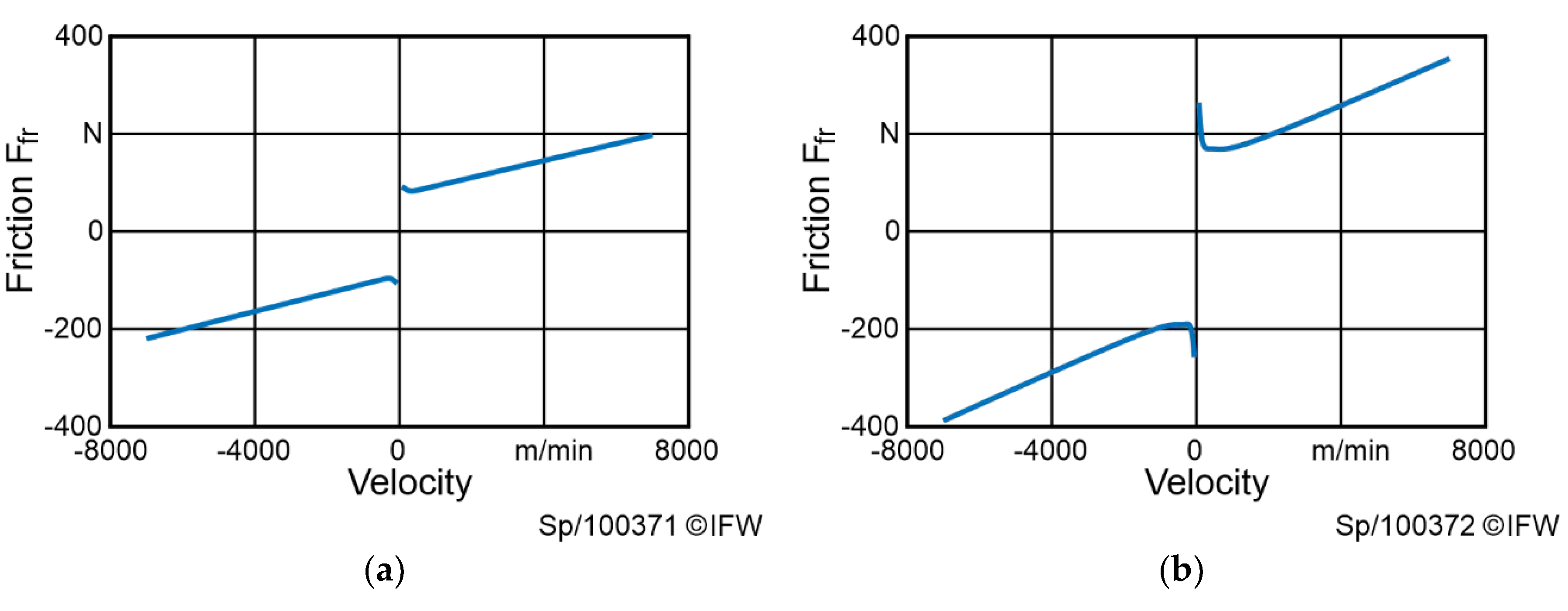
Third, the friction is reconstructed by a Stribeck curve, described by Equation (4) [18].
F f r ( s ˙ ) = s g n ( s ˙ ) · ( F C + ( F b r F C ) e | s ˙ v s | δ ) + σ s ˙
Hence, five parameters have to be adjusted. According to Ruderman [18], the Stribeck shape factor δ can be assumed as δ = 2 . Breakaway friction F b r , Coulomb friction F C , Stribeck velocity threshold v s , and viscous friction coefficient σ are subject to an optimization. To this end, axis slide movements are performed, covering a range of constant velocities. Since F c o ( s ) and F s ( s ) have been determined before, both are subtracted from the motor force, as expressed in Equation (5).
F ˜ f r = K m · I F c o ( s ) k · ( s s r )  
Since position dependent effects have been compensated, the remaining signal F ˜ f r is mostly due to friction and depends on the velocity s ˙ . Optimal friction parameters are then determined by finding the minimal nonlinear least squares error E f r compared to the recorded data using the ‘trust-region-reflective’ algorithm, outlined in Equation (6). The results are shown in Figure 2.
E f r =   s ˙ ( F ˜ f r ( s ˙ ) F f r ( s ˙ ) ) 2
Finally, the mass parameters for the calculation of forces of inertia are determined. For this purpose, accelerated movements are considered and frictional, cogging as well as restoring forces are eliminated from the recorded signal. The mass parameters m x , m y , and m z are calculated by minimizing the least squares error E m , s , regarding Equations (7)–(10).
F ˜ m , s = K m · I F c o ( s ) k · ( s s r ) F f r ( s ˙ )  
E m , x =   x ¨ ( F ˜ m , x ( x ¨ ) ( m x + m z ) x ¨ ) 2
E m , y =   y ¨ ( F ˜ m , y ( y ¨ ) ( m x + m y + m z ) y ¨ ) 2
E m , z =   z ¨ ( F ˜ m , z ( z ¨ ) m z z ¨ ) 2
All four steps are repeated for each axis. The above described model states a model-based reference to compare with the presented LSTM.

2.3. Neural Network Based Force Reconstruction

The neural network designed and evaluated in this work is based on the LSTM, developed by Hochreiter and Schmidhuber [19]. The LSTM is especially useful to predict time series, since every LSTM cell passes its inner state c ( t ) forth to the next iteration [20]. The LSTM cell used in this work as a building block is similar to the LSTM cell used in a study by Lipton and colleagues [21]. In particular, no peepholes are used (compare [20] and [22]). According to Lipton and colleagues [21], the LSTM cell is defined by Equations (11)–(16), where σ is the sigmoid function, W is a weight matrix, and b is the bias. W and b are specific to each equation and therefore marked with the corresponding index f , g , i or o . The dimensions of W and b are subject to the hyperparameter optimization, while the individual elements are a result of the training. x ( t ) is the input delivered by the previous layer. In every iteration the LSTM discards a proportion of the old state c ( t 1 ) depending on a forget gate f ( t ) (Equation (11)). Analog an input gate i ( t ) is used to keep a proportion of a new calculated cell state candidate g ( t ) (Equations (12) and (13)). The cell state is updated by combining the old cell state and the candidate according to Equation (15). The output h ( t ) of a LSTM cell is calculated from the Hadamard product of the output gate o ( t ) and the hyperbolic tangens of the cell state (Equations (14) and (16)).
f ( t ) = σ ( W f , h · h ( t 1 ) + W f , x · x ( t ) + b f )  
g ( t ) = t a n h ( W g , h · h ( t 1 ) + W g , x · x ( t ) + b g )  
i ( t ) = σ ( W i , h · h ( t 1 ) + W i , x · x ( t ) + b i )  
o ( t ) = σ ( W o , h · h ( t 1 ) + W o , x · x ( t ) + b o )  
c ( t ) = c ( t 1 ) f ( t ) + g ( t ) i ( t )  
h ( t ) = o ( t ) tan h ( c ( t ) )  
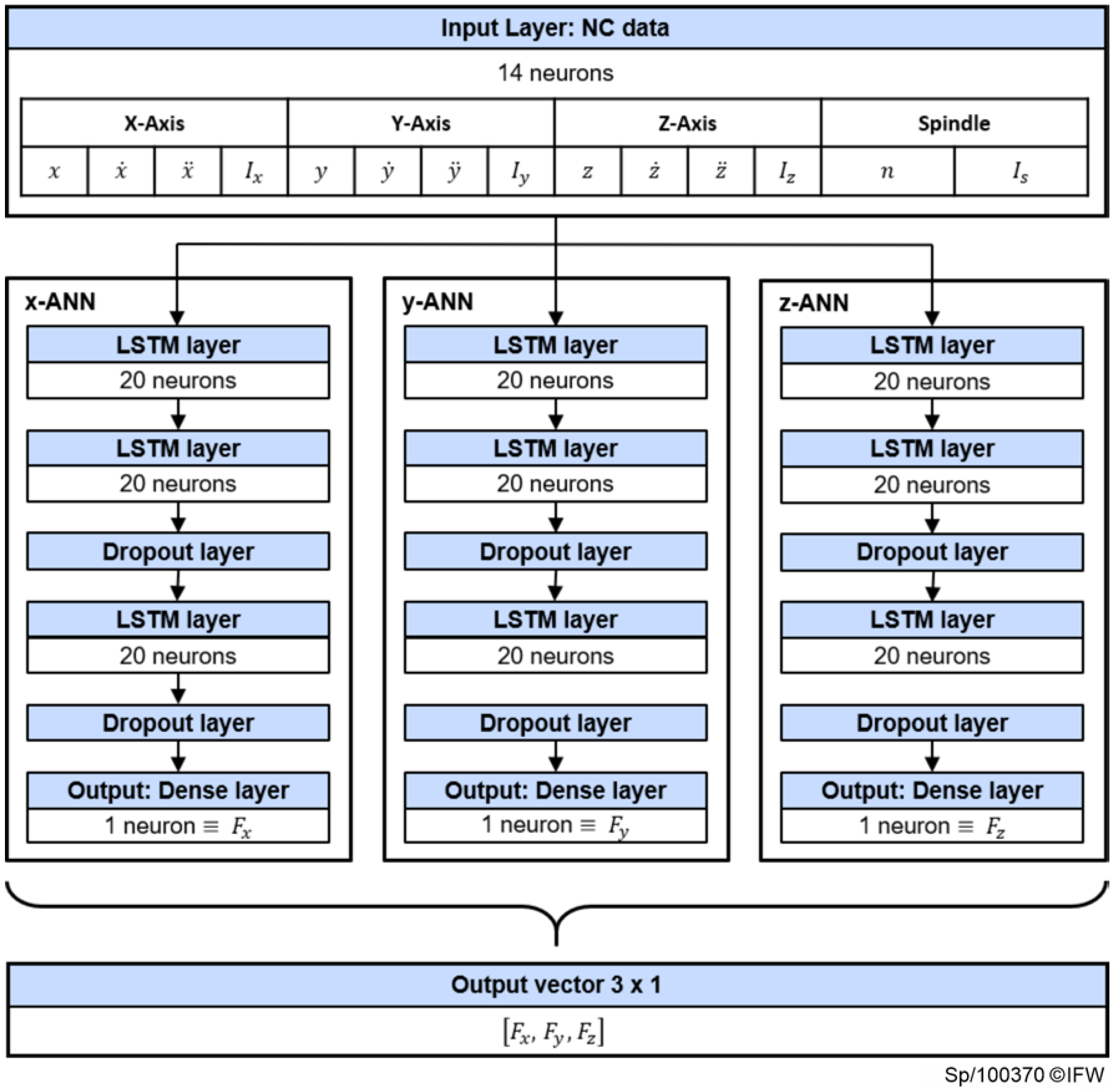
The developed network is presented in Figure 3. Its input neurons correspond to the control data of the Sinumerik 840D sl. In particular, these are the axis positions, velocities, accelerations, and motor currents of the X-, Y-, and Z-axis as well as the spindle speed and the motor current of the spindle. The input layer is connected to a layer consisting of 20 LSTM cells followed by two more LSTM layers by the same size. Finally, the output layer is formed by a single neuron, representing one of the force components in the X-, Y-, and Z-direction. Consequently, each force component is decoupled with its own sub-ANN. The design of the neural network results in an iterative process performed on a subset of the training data. Based on this subset it was found that three separate LSTMs converged faster than a single network reconstructing all three force components at once. To avoid overfitting, dropout is used during the training of the network [23].
Coming to train the network, quantity and quality of the underlying data are very important. A higher amount of training data reduces the risk of overfitting. As explained in Section 2.1, the data is collected by recording drive data as well as force measurements from a plate dynamometer during the milling process. A zero-phase Butterworth filter with a cutoff frequency of 120 Hz is applied to the force measurement data. The cutoff frequency is chosen with respect to the Nyquist–Shannon sampling theorem. Due to the sampling rate of the streamed NC data (250 Hz), no higher frequencies than 125 Hz can be reconstructed from the signal. Afterwards, the force measurements are scaled and shifted according to Equation (17). Thereby, the new calculated force F i * is one for the highest ever measured absolute value | F i m a x | with i   { x , y , z } . Moreover F i ( k ) = 0 corresponds to F i * ( k ) = 0.5 after transformation.
F i * ( k ) = F i ( k ) 2 · | F i m a x | + 0.5                   F i ( k )     F i :   | F i m a x |       | F i ( k ) |  
To a small extent, this preprocessing approach deviates from standard normalization techniques like Min-Max Feature Scaling. The new approach achieves a faster convergence of the training loss compared to standardization with zero mean and regular normalization. However, the normalization technique is specific to the use case. The drive data remain unfiltered and are normalized to a range of [−1, 1] or rather [0, 1] for strictly positive variables like the position.
An important aspect is the variation of the process parameters while recording the measurements. For classification tasks it has been shown that the data should be evenly distributed, by the means that no class should be underrepresented in the dataset [24]. Since regression is a different task, transferring this knowledge from classification data sets to the use case of force reconstruction is not trivial. Every neural network has to be considered as a black box model. Hence, there is no rule, constraining the network to learn the process forces based on physical laws. As already pointed out for the model-based approach, different forces affect the behavior of the linear drives. Thus, it is not sufficient to teach a neural network only with data collected from milling straight grooves, because given a constant feed rate, no acceleration occurs. On the other hand, teaching only records of circular pocket milling, would not provide necessary information on how the process force behaves, if feed rates are constant. For best results a broad range of processes and process parameters should be considered to prevent the neural network from overfitting. In addition to the influence of different processes to the linear drive, the acting process forces need to be varied. According to Kienzle [25], the process forces depend on the tool, the workpiece material, and the machining conditions. Tool and material are not the subject of this study, so only the machining conditions are varied. In particular, these are cutting speed, which depends on spindle speed n and tool diameter, feed rate vf, depth of cut ap, and width of cut ae. Table 1 gives a full overview of the variations of the process parameters for the training data. Based on the tool manufacturer’s data, these variations where determined by preliminary tests.
For the dataset only parameter combinations are considered which result in undisturbed milling processes; for example, the measurement was not taken into account when chatter was detected. All in all, 181 parameter variations were considered. In total, 160 of these recorded datasets were used for training. The other 21 datasets are not shown to the network while training and were used as test data.

3. Results

Both the model-based approach as well as the LSTM are capable of reconstructing process forces. Nevertheless, they have different advantages and disadvantages. Subsequently, the two approaches are evaluated based on various processes. In detail these are side and groove milling processes with different feed directions, milling of a circular pocket, and ramp milling.

3.1. Model-Based Force Reconstruction

Since the model-based approach does not need any force measurements for parametrization, it is not necessary to discriminate between train and test datasets. All force measurements are unknown to the model. Hereafter, the model is evaluated using representative examples. The focus of the evaluation is on the reconstruction of the X- and Y-axis. In Figure 4, the measured and the reconstructed forces of a slot milling process with diagonal feed direction in the X/Y-plane with a material recess (t = 10.5 s to t = 12.5 s) are shown. The deviation between reconstructed and measured force is very small, with a root mean square error (RMSE) of 32.95 N for the X-component and a RMSE of 20.87 N for the Y-component of the force. It stands out, that at the beginning and at the end of the milling process, there are peaks in the reconstructed force signal, when the movement sets in. Those are due to the stiction and the characteristic of the implemented Stribeck model. Moreover, a closer look at Figure 4b from t = 6 s to t = 10 s as well as Figure 5a from t = 4 s to t = 10 s, reveals that there are some oscillations with a very low frequency of around 0.2 Hz. In relation to the axis position, this results in a distance of 23 mm for one period which corresponds to the pole width of the linear drive. This suggests that the oscillations are due to the motor cogging, which is not fully compensated by the model for the given process parameters. However, there also have been trials, where a too-high cogging compensation induced oscillations.
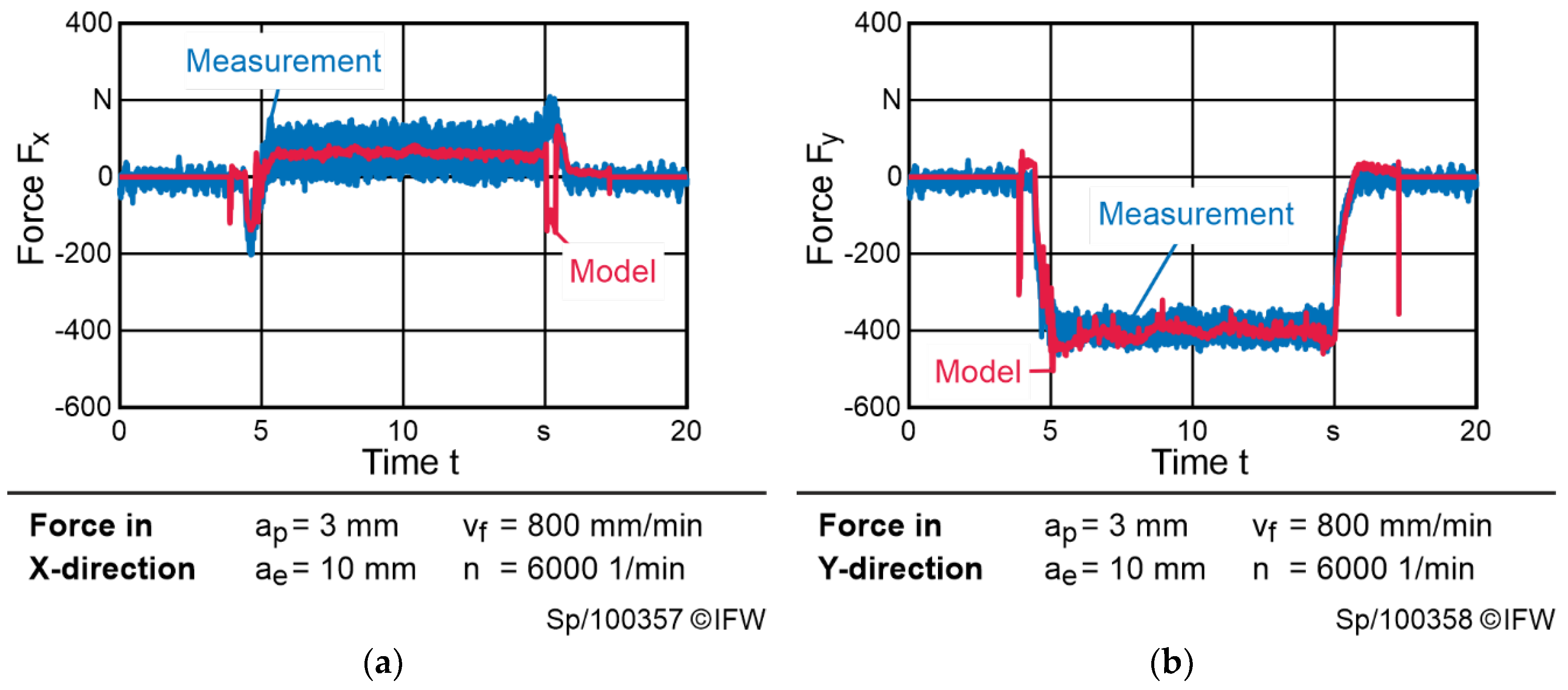
Altering the process parameters, again the model achieves a RMSE lower than 40 N (see Figure 5). Nevertheless, a constantly higher force is reconstructed by the model. This effect can be interpreted as a systematical error, caused by the deliberately low model complexity. Further investigations could minimize these errors. For example, friction parameters could be adapted regarding different axis positions, as wear might cause different surface quality of the guidance. Yet with higher complexity the model is increasingly susceptible to overfitting.
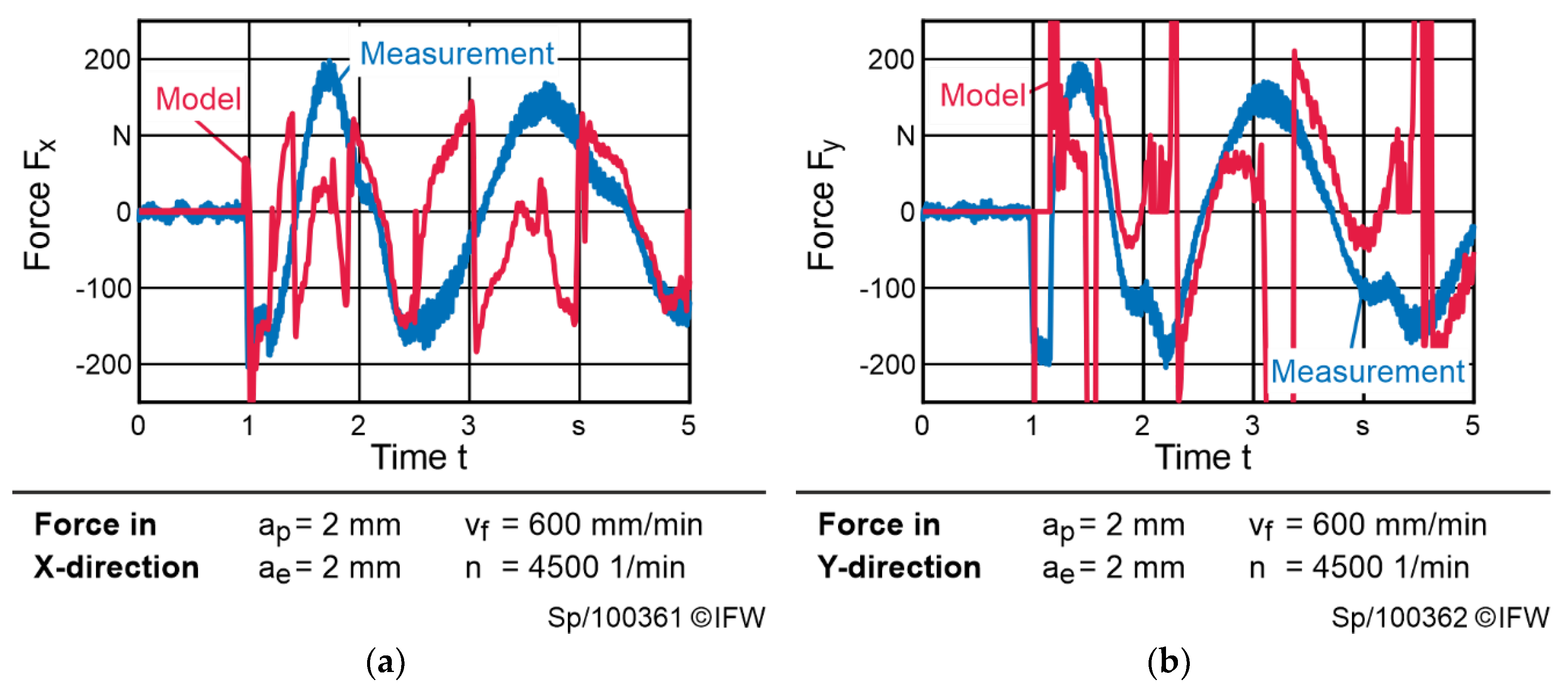
Figure 6 shows a pocket milling process. Here, the limitations of the model-based approach become apparent; especially when the direction of a feed axis is changing, there is a poor model quality. The combination of accelerated axis and micro friction clearly is one of the major drawbacks of the model.

3.2. LSTM

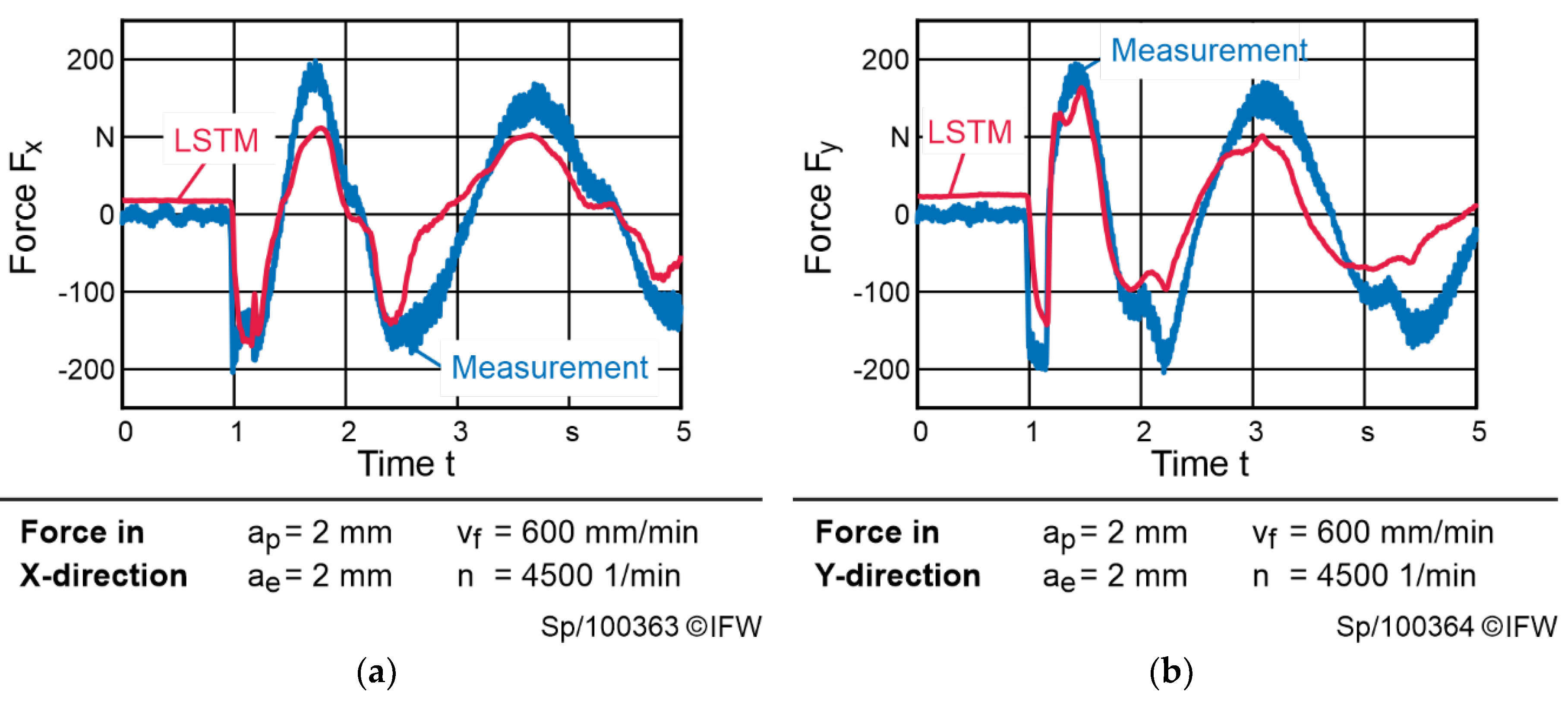
For the evaluation of the LSTM a test set is used, which has not been introduced to the network before. Like the previously evaluated model-based approaches, the LSTM leads to good results as well. When milling circular pockets, the forces can be reconstructed better, compared to the model-based approach (see Figure 7). Even the first peak, marking the transition between drilling and milling operation at the beginning of a pocket milling process is reconstructed. Nevertheless, the reconstructed signal still deviates from the measurement. In particular, negative forces are reconstructed with a minor quality, which leads to a RMSE of 49.8 N in the X-direction and 38.3 N in the Y-direction.
Analyzing the RMSE and comparing it to the model-based approach, in most cases the LSTM outperforms the model-based approach. An overview of the RMSE of both models is given in Table 2, showing different evaluated milling processes of the test set. The test set covers straight side milling processes with different process parameters as well as ramp milling (indicated with the −y/+z feed direction) and circular pocket milling with a counterclockwise (ccw) feed direction.
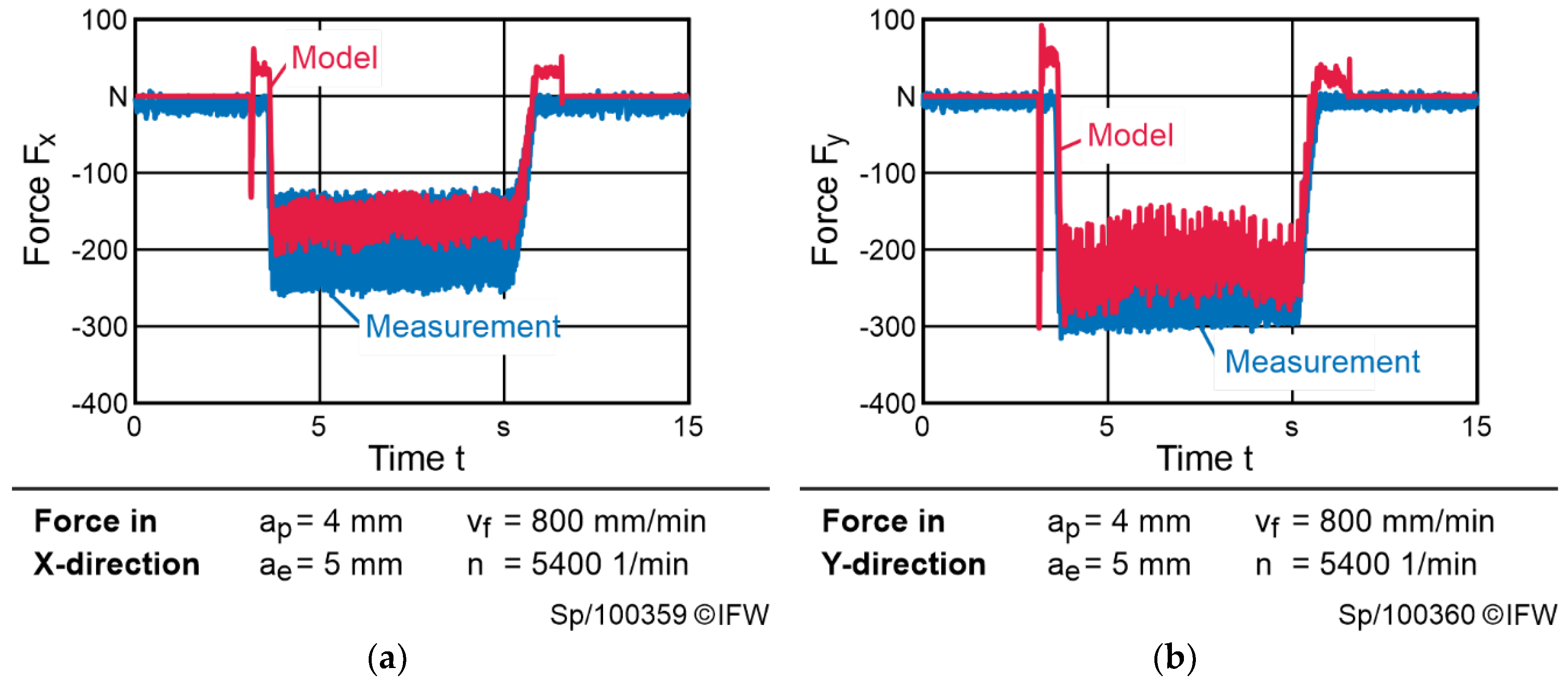
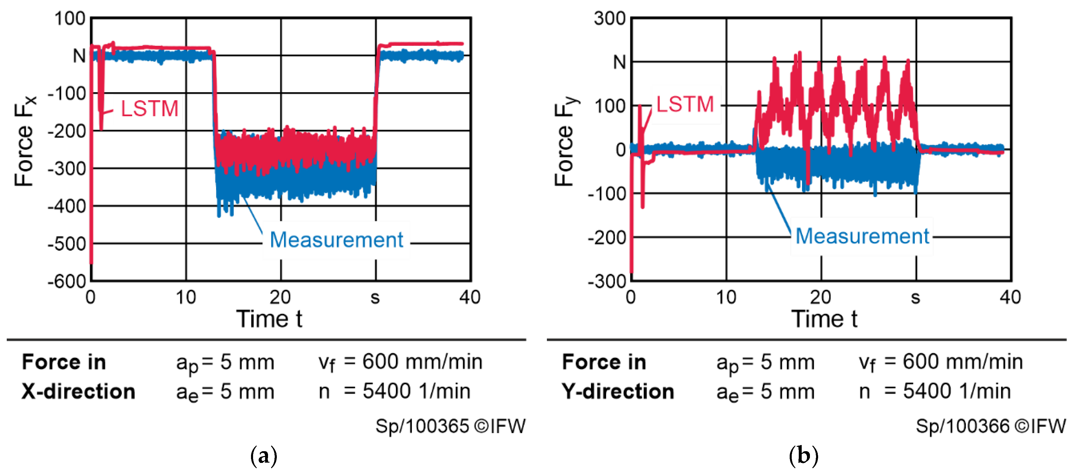
Averaged over the test set, the RMSE of the LSTM is 20.8% lower than the RMSE of the model-based approach. For many processes the LSTM reconstructs the forces with a RMSE of approximately 35 N. The median RMSE for all processes and axes is 35.3 N. However, some outliers occur in certain applications and leverage the overall RMSE of the LSTM to 50.2 N. One of those outliers can be inspected in Figure 8. While the forces in the X-direction are reconstructed sufficiently with a RMSE of 48.7 N, the LSTM reconstructs an oscillating force in the Y-direction leading to a RMSE of 88.6 N. More detailed investigations show high frequent oscillations of the Y-axis velocity, indicating a semi-stable process. Since instable processes have been discarded, semi-stable processes indicate a high difference between measured process variables and desired set points. Compared to the model-based approach with a RMSE of 245.3 N in the Y-direction, the LSTM still reconstructs the force more accurately. The same applies to other semi-stable processes (see Table 2, line 3).
In the case of the ramp milling process the RMSE is 25.1, which is lower than average (Figure 9). Nevertheless, the LSTM reconstructs some characteristic oscillations which do not correlate with the force measurement. Similar oscillations already occurred during training. Since the oscillations have a moderate amplitude, they do result in a RMSE. As a consequence, unlearning them by minimizing the RMSE is difficult. Possible reasons for the oscillating output of the LSTM are oscillations in the input signal and the LSTM itself, but further investigations need to be conducted.

4. Conclusions and Outlook

This work presents two approaches to reconstruct the process forces from the drive signals, including the motor current. Both approaches show a sufficient accuracy for the reconstruction of the process forces. Nevertheless, the LSTM is more robust when the axis accelerates during machining. Here, the LSTM achieves a higher accuracy in comparison to the model-based approach. Overall, the RMSE of the LSTM is lower than the RMSE of the model-based approach. The investigations have also shown that the reconstruction of forces based on the drive currents is highly dependent on the process. Thus, a RMSE of 12 N could be achieved for individual axes. Other processes led to RMSEs of more than 100 N. Process stability is especially essential for the performance of both approaches, but the model-based approach is much more affected by a decreasing process stability. As a consequence, outliers occur more often and lead to even higher errors. Since some outliers occur simultaneously in both approaches, this is an indication that in these cases there are limitations to reconstruct the forces based on the drive current. In order to analyze this more precisely, the complexity of both approaches must be examined on the one hand and the quality of the signal on the other.
Even though in some cases it seems rather obvious that a neural network trained only on selected data does not generalize to new processes, it is difficult to rate whether the recorded data are sufficient or not. In this work a broad range of different machining conditions is covered for training data. It has been shown that processes with constant feed velocity as well as accelerated axis feed are necessary to train a robust and generalizable network. Taking this into account a high degree of generalizability is achieved by the presented LSTM.
Compared to other neural networks (see [13]) the presented one does not learn a material removal simulation, but estimates the transfer functions of the direct drives, fused with spindle data. From this the hypothesis can be deduced that not all workpiece materials and tool variations are necessary for the training data. Instead, the operating range of the motors needs to be covered, which might be easier to achieve. To prove this hypothesis, different milling tools, tool holders, and workpiece materials should be evaluated in following studies. Thereby, the network would be enabled to react to material inhomogeneities, which could not be considered by simulations.
Furthermore, neural networks have to be considered as black box models. Therefore, it is desirable to extend the network in a way that predictions can be made regarding the uncertainty of the reconstructed process force. In conclusion, neural networks in general, and the presented LSTM in particular, are highly suitable to reconstruct process forces, but higher effort in generating training data for a well-trained network is necessary.

Author Contributions

Conceptualization, D.S. and B.B.; methodology, D.S.; software, D.S.; validation, D.S.; formal analysis, D.S.; investigation, D.S.; resources, D.S.; data curation, D.S.; writing—Original draft preparation, D.S.; writing—Review and editing, B.D. and B.B.; visualization, D.S.; supervision, B.D. and B.B.; project administration, D.S.; funding acquisition, B.D. All authors have read and agreed to the published version of the manuscript.

Funding

This research was funded by the German Research Foundation (DFG), grant number DE447/160-1.

Acknowledgments

We thank the DFG for funding this project and our project partner DECKEL MAHO Seebach GmbH.

Conflicts of Interest

The authors declare no conflict of interest.

References

  1. Altintas, Y. Prediction of Cutting Forces and Tool Breakage in Milling from Feed Drive Current Measurements. J. Eng. Ind. 1992, 114, 386–392. [Google Scholar] [CrossRef]
  2. Plapper, V.; Weck, M. Sensorless machine tool condition monitoring based on open NCs. In Proceedings of the 2001 ICRA IEEE International Conference on Robotics and Automation (Cat. No.01CH37164), Seoul, Korea, 21–26 May 2001; Volume 3, pp. 3104–3108. [Google Scholar]
  3. Cus, F.; Zuperl, U. Model reference-based machining force and surface roughness control. J. Achiev. Mater. Manuf. Eng. 2008, 29, 115–122. [Google Scholar]
  4. Dow, T.A.; Miller, E.L.; Garrard, K. Tool force and deflection compensation for small milling tools. Precis. Eng. 2004, 28, 31–45. [Google Scholar] [CrossRef]
  5. Denkena, B.; Dahlmann, D.; Boujnah, H. Tool Deflection Control by a Sensory Spindle Slide for Milling Machine Tools. Procedia CIRP 2017, 62, 329–334. [Google Scholar] [CrossRef] [Green Version]
  6. Miura, K.; Döbbeler, B.; Klocke, F. Cutting power estimation via external voltage and current sensors on feed-drive axis for the straight milling process. Procedia CIRP 2018, 78, 323–328. [Google Scholar] [CrossRef]
  7. Schwenzer, M.; Auerbach, T.; Miura, K.; Döbbeler, B.; Bergs, T. Support vector regression to correct motor current of machine tool drives. J. Intell. Manuf. 2020, 31, 553–560. [Google Scholar] [CrossRef]
  8. Yamada, Y.; Kakinuma, Y. Sensorless cutting force estimation for full-closed controlled ball-screw-driven stage. Int. J. Adv. Manuf. Technol. 2016, 87, 3337–3348. [Google Scholar] [CrossRef]
  9. Yamada, Y.; Yamato, S.; Kakinuma, Y. Mode decoupled and sensorless cutting force monitoring based on multi-encoder. Int J. Adv. Manuf. Technol. 2017, 92, 4081–4093. [Google Scholar] [CrossRef]
  10. Aslan, D.; Altintas, Y. Prediction of Cutting Forces in Five-Axis Milling Using Feed Drive Current Measurements. IEEE/ASME Trans. Mechatron. 2018, 23, 833–844. [Google Scholar] [CrossRef]
  11. Jeong, Y.-H.; Cho, D.-W. Estimating cutting force from rotating and stationary feed motor currents on a milling machine. Int. J. Mach. Tools Manuf. 2002, 42, 1559–1566. [Google Scholar] [CrossRef]
  12. Kim, T.-Y.; Woo, J.; Shin, D.; Kim, J. Indirect cutting force measurementnin multi-axis simultaneous NC milling process. Int. J. Mach. Tools Manuf. 1999, 39, 1717–1731. [Google Scholar] [CrossRef]
  13. Königs, M.; Wellmann, F.; Wiesch, M.; Epple, A.; Brecher, C.; Schmitt, R.; Schuh, G. A scalable, hybrid learning approach to process-parallel estimation of cutting forces in milling applications. Robert Schmitt Günther Schuh (Publ.) 2017, 7, 425–432. [Google Scholar]
  14. Zagórski, I.; Kulisz, M.; Semeniuk, A. Artificial Neural Network Modelling of Cutting Force Components in Milling; EDP Sciences: Les Ulis, France, 2017; Volume 15, p. 02001. [Google Scholar]
  15. Zuperl, U. Cus, Franc Adaptive Network Based Inference System for Cutting Force Simulation in Milling of Multi-Layered Metal Materials. Proc. Manuf. Syst. 2017, 12, 47–52. [Google Scholar]
  16. Matlab. Available online: https://www.mathworks.com/products/matlab.html (accessed on 1 July 2020).
  17. Albrecht, A. Wärmedehnungskompensierte Rekonstruktion von Prozesskräften an Vorschubantrieben. Ph.D. Thesis, Technische Universität Braunschweig, Braunschweig, Germany, 2009. [Google Scholar]
  18. Ruderman, M. Zur Modellierung und Kompensation dynamischer Reibung in Aktuatorsystemen. Ph.D. Thesis, Technische Universität Dortmund, Dortmund, Germany, 2012. [Google Scholar]
  19. Hochreiter, S.; Schmidhuber, J. Long Short-Term Memory. Neural Comput. 1997, 9, 1735–1780. [Google Scholar] [CrossRef] [PubMed]
  20. Greff, K.; Srivastava, R.K.; Koutnik, J.; Steunebrink, B.R.; Schmidhuber, J. LSTM: A Search Space Odyssey. IEEE Trans. Neural Netw. Learn. Syst. 2017, 28, 2222–2232. [Google Scholar] [CrossRef] [PubMed] [Green Version]
  21. Lipton, Z.C.; Kale, D.C.; Elkan, C.; Wetzel, R. Learning to Diagnose with LSTM Recurrent Neural Networks. arXiv 2017, arXiv:1511.03677. [Google Scholar]
  22. Gers, F.A.; Schmidhuber, J. Recurrent nets that time and count. In Proceedings of the IEEE-INNS-ENNS International Joint Conference on Neural Networks. IJCNN 2000. Neural Computing: New Challenges and Perspectives for the New Millennium, Como, Italy, 27 July 2000; Volume 3, pp. 189–194. [Google Scholar]
  23. Srivastava, N.; Hinton, G.; Krizhevsky, A.; Sutskever, I.; Salakhutdinov, R. Dropout: A simple way to prevent neural networks from overfitting. J. Mach. Learn. Res. 2014, 15, 1929–1958. [Google Scholar]
  24. Zhu, X.; Vondrick, C.; Ramanan, D.; Fowlkes, C.C. Do We Need More Training Data or Better Models for Object Detection; Citeseer: University Park, PA, USA, 2012; Volume 3. [Google Scholar]
  25. Kienzle, O. Die bestimmung von kräften und Leistungen an spanenden Werkzeugen und Werkzeugmaschinen. VDI-Z 1952, 94, 299–305. [Google Scholar]
Figure 1. Model-based approach: (a) complete model; (b) X-axis submodel.
Jmmp 04 00062 g001
Figure 2. Stribeck curve: (a) fitted for the X-axis of the HSC30; (b) fitted for the Y-axis of the HSC30.
Jmmp 04 00062 g002
Figure 3. Schema of the long short-term memory neural network (LSTM) neural network.
Jmmp 04 00062 g003
Figure 4. Comparison between measured process forces and the model-based approach during milling of a diagonal groove: (a) force acting in X-direction (root mean square error (RMSE) = 36.22 N); (b) force acting in Y-direction (RMSE = 28.25 N).
Jmmp 04 00062 g004
Figure 5. Comparison between measured process forces and the model-based approach during milling of a diagonal groove: (a) force acting in X-direction (RMSE = 30.74 N); (b) force acting in Y-direction (RMSE = 33.49 N).
Jmmp 04 00062 g005
Figure 6. Comparison between measured process forces and the model-based approach during milling of a circular pocket: (a) force acting in X-direction (RMSE = 104.4 N); (b) force acting in Y-direction (RMSE = 149.1 N).
Jmmp 04 00062 g006
Figure 7. Comparison between measured process forces and the result of the LSTM during milling of a circular pocket: (a) force acting in X-direction; (b) force acting in Y-direction.
Jmmp 04 00062 g007
Figure 8. Comparison between measured process forces and the result of the LSTM during side milling in negative X-direction: (a) force acting in X-direction; (b) force acting in Y-direction.
Jmmp 04 00062 g008
Figure 9. Comparison between measured process forces and the result of the LSTM during ramp milling in negative Y-direction and positive Z-direction: (a) force acting in X-direction; (b) force acting in Y-direction.
Jmmp 04 00062 g009
Table 1. Overview of process variations of recorded training data.
ParameterUnitVariations
ap(mm){1, 2, 3, 4}
ae(mm){1, 2, 4, 5, 7, 10}
vf(mm/min){300, 400, 500, 700, 800}
n(1/min){2600, 3500, 4500, 5400, 6000}
Table 2. RMSE of the LSTM compared to the model-based approach and the measured forces Fme.
Feed DirectionaeapfnANNModelMax. |Fme|
x|yx|yx|y
(mm)(mm)(mm/min)(1/min)(N)(N)(N)
+x52800540033.9|12.018.9|132.8238.7|117.6
+x52800600036.6|33.268.8|29.5222.6|144.6
+x558005400146.0|58.6128.9|772.7448.5|146.1
+x72400260077.9|101.353.6|536.01016.7|740.5
+x72800540036.8|29.231.5|225.1372.6|208.3
+x72800540033.8|25.430.1|127.0241.1|166.8
+x101700500035.6|54.823.3|129.4375.0|317.8
−x52600540030.1|22.645.0|51.580.8|212.3
−x53800600042.7|27.732.8|30.3100.4|320.9
−x103800500034.3|19.512.9|26.8268.5|536.9
−y55600540048.7|88.699.0|245.3478.8|281.5
−y101300260048.5|74.1157.4|179.0579.6|634.4
−y101500350042.5|81.190.5|172.4836.0|709.6
+x/−y52600450038.9|23.112.0|153.7205.4|458.0
+x/−y54800540036.9|31.130.7|33.5261.3|314.25
+x/−y101600540032.6|26.223.9|67.299.3|208.6
−x/+y53600450068.6|26.6157.1|26.3324.9|544.3
−x/+y54800600036.5|21.564.4|54.4297.4|246.0
−x/+y102600540035.0|32.147.7|163.4156.6|321.5
−y/+z100 to 2600500028.1|21.450.6|18.2206.2|115.5
ccw22600450049.8|38.3104.4|149.1247.5|437.0
Abbreviations: ANN = artificial neural network; ccw = counterclockwise.